Happiness Index Determination by Analyzing Satellite Images for Urbanization

ABSTRACT

Waterbody identification from satellite images in an automated manner is one of the difficult tasks in the domain of Remote Sensing (RS). In recent years, several image processing approaches have been developed to process RGB or multispectral images to analyze the availability of land, water prediction, object detection, climate change, LULC, and many others. In this study, a Multi-data Fusion Network (MDFN) is developed to extract the sources of water by utilizing Sentinel-2 satellite images. The spatial features are extracted by proposed model from RS images by comprising multiple structural learning-assisted feature fusion layers for water resource prediction. To justify the prediction performance, the calculated outcomes of developed solution are correlated with the other approaches such as DeepLabv3+, VGG, NDWI, SegNet, DenseNet, and ResNet. The calculated outcomes define the prediction superiority over the other models by registering the high value of Precision, F1-score, Recall, and IoU with the value of 0.958%, 0.928%, 0.899%, and 0.874%, respectively.

Introduction

The utilization of satellite images to map natural resources such as forests and water bodies has become increasingly popular in recent years. Forest and water resources are heavily used; therefore, regular monitoring is essential for the long-term management of these resources. The industrial revolution brought the large need for water that causes the problem of global warming and climate change. This development generates the need to identify the source water bodies in a persistent way to estimate the quantity and quality of water resources (Famiglietti and Rodell 2013; Feng et al. 2015). Moreover, the continuous growth of industries also causes the change of urbanization that claim the improper control of water conservation (Xie et al. 2018; N. Du, Ottens, and Sliuzas 2010; Shuster et al. 2005; X. Yang et al. 2017). In this manner, an actual and accurate view of urban sources of water is critical for the development of sustainability.

Problem Identification and Motivation

Recognition of water bodies in a precise manner from satellite images is considered one of the important applications in the domain of environment monitoring. Different water prediction techniques have been developed in previous studies for resolving the issue of water index misclassification. However, accurately assessing the dynamics of water spectral features from a series of images is challenging due to the complex properties of water spectral reflectance (Fisher, Flood, and Danaher 2016). In this manner, water index methods have been misclassified by the majority of the traditional approaches. Therefore, several limitations have been identified and presented in Table 1 in terms of water bodies recognization.

Table 1. Comparison of multiple parameters

Studies	Fining	Satellite data	Type of data	Fog platform	Cloud platform	Techniques	Real-time
Feyisa et al. 2014	An automatic water extraction index is proposed to enhance the water extraction accuracy while taking into consideration of various types of environmental noise	Yes	NIR	No	No	Conventioanl	No
McFeeters 1996	The NDWI approach is proposed to extract the aource of water from satellite images	Yes	NIR	No	No	Conventioanl	No
Kang et al. 2016	Empirical evaluation is conducted on VIIR data for surface water detection	Yes	SWIR	No	No	Conventioanl	No
Xu 2006	The modified NDWI called MNDWI is proposed to enhance the open water features	Yes	NIR	No	No	Conventioanl	No
Kang et al. 2016	Multireservoir is identifies by developing Hybrid approach	Yes	-	No	No	Conventioanl	No
Zhang et al. 2016	In this study these issues are discussed 1) Remote sensing classification, 2) Change detection, 3) Fusion of diverse images	Yes	SAR	No	No	Advanced	No
Fang et al. 2019	The CNN-based framework is developed for the detection of reservoir	Yes	Multispectral Bands	No	No	Advanced	No
Chen et al. 2018	The identification water resources from satellite images are evaluated by developing deep learning approach	Yes	False-color composite	No	No	Advanced	No
Yu et al. 2017	To extract water from landsat 8 data, a hybrid technique based on deep learning is presented	Yes	Spectral bands	No	No	Advanced	No
Isikdogan, Bovik, and Passalacqua 2017	Fully convolutional neural network is designed that specifically used to segment the water from landsat-8 images	Yes	All reflective bands	No	No	Advanced	No
Tambe, Talbar, and Chavan 2021	Multi features-based CNN is designed to perform the task of water body segmentation.	Yes	Spectral Images	No	No	Asvanced	No
Proposed Solution	A new Multi-scale Data Fusion Network (MDFN) is presented in this proposed study to segment the water resources from a desired area.	Yes	False-Color Composite	Yes	Yes	Advanced	Yes

Contribution

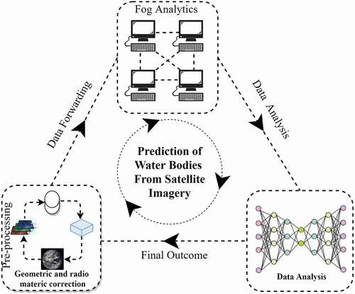
Water extraction methods employ standard procedures to acquire data about water availability using remote sensing images (Y. Afaq and Manocha 2021a; Du et al. 2016; Wu et al. 2019; Zhou et al. 2014; Afaq and Manocha 2021b). By following the need of analyzing the water resource, the proposed solution has utilized RS images as illustrated in Figure 1. Moreover, it has been analyzed that forwarding the data to the cloud is increasing the transmission cost with latency. However, Fog computing is considered one of the most effective solutions to deal with these two parameters (Manocha et al. 2020). In this manner, the fog layer helps to achieve the distributed computing environment by processing the data near to the user. To fulfill the objective of the study, the contributions of the proposed study are listed as:

1. To develop Deep Convo-Restrictive Model for covering the large targeted area by analyzing the structural relationships among the smaller area.

2. To add Conditional Random Field (CRF) layer in the proposed MDFN to enhance the process of inferencing.

3. To improve spatial inferences by utilizing the Spatial-Inferred-Features (SIF) to calculate the information of the targeted region for a significant representation.

4. To transfer features to the Deep-Sparse-Auto-encoder (DSA) module and calculate non-linear connection from local and global data.

Figure 1. Conceptual framework for water bodies identification from satellite imagery.

Article Organization

The remaining article is structured into different sections and subsections. Section 2 is devoted to a survey of the major literature on conventional and advanced techniques for water identification. In Section 3, every potential element of the suggested architecture is examined. The experimental outcomes are presented in Section 4. Lastly, in Section 5, the conclusion of the proposed solution and future perspective of the proposed study is discussed.

Literature Review

Several solutions have been introduced to evaluate water bodies using remote sensing data by utilizing sub-pixels (Li et al. 2015; Yan et al. 2018) . The previously developed solutions are divided into two following categories: (i) Conventional approaches and (ii) Advanced approaches.

Conventional Approaches

Researchers have suggested several ML approaches such as SVM, k-means clustering, and many others to evaluate RS images with different resolutions (Kang et al. 2016; Katz 2016; Huang et al., 2015) and the selection of important features is critical in these proposed techniques from RS images. The hand-crafting process for the collection of spatial features by using such methods is laborious and time-consuming (Kang et al. 2016). McFeeters (1996) proposed an NDWI approach for analyzing the target objects. This model has a limitation in terms of gap analysis among shadows and water sources. To improvise the performance of the NDWI model, author Xu (2006) recommended an infrared band instead of the green band to easily differentiate the shadows and water from satellite images. The method yielded the best results for urban water bodies identification.

Advanced Methods

In RS applications, deep learning has overcome the limitation of previously developed image processing techniques (Ma et al. 2019; Zhang et al. 2016; Zhu et al. 2017; Lee et al., 2009). The Convolutional Neural Network (CNN) is widely used for obtaining spatial characteristics (Y. Han et al. 2020). CNN has a potential to extract multi-level characteristics. The potential of the extraction of multi-level characteristics is the major asset of the CNN approach. Weinstein and Ebert proposed MFCN which was upgraded by adding Fully Convolutional Network (FCN) (Weinstein and Ebert 1971) to extract multiscale features for water extraction (Afaq and Manocha 2021a; Geng et al. 2020). CNN has been utilized by certain researchers to monitor the source of water from multi-resolution satellite images. In this manner, the findings show that CNN has the capability to differentiate water area and ground shadows (Chen et al. 2018; Fang et al. 2019; Isikdogan, Bovik, and Passalacqua 2017; Yu et al. 2017). Li et al. (2018) proposed a novel DeepUNet model based on Convolution Neural Network to segment pixels of an image to differentiate sea water. Furthermore, the semantic segmentation with extended DeepLabv3+ was utilized on cityscapes dataset with different parameters (Yurtkulu, Sahin, and Unal 2019). Lately, a novel DeepWaterMapV2 was proposed to map the surface water at a lower cost with improved precision and recall value (Isikdogan, Bovik, and Passalacqua 2019).

As significant research toward this path has been observed, researchers have tried to incorporate advanced approaches for the effective prediction of natural resources from satellite images. However, several limitations have been observed and listed in Table 1. To overcome those limitations and gaps, this research is aiming to develop a robust solution for the prediction of water from RS data.

Proposed Methodology

The proposed study aims to segment different water resources by utilizing data processing and handling principles of deep learning and fog analytics. Every possible aspect of the proposed MDFN is explained by dividing it into three phases as Data Acquisition and Image pre-processing, Water resource determination, and Degree of happiness index determination as illustrated in Figure 2.

Figure 2. Complete process of proposed MDFN.

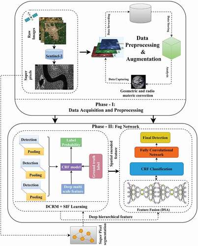
Data Acquisition and Pre-processing

As Punjab is considered as an essential food production state in India (Kumar and Kumari 2020), the availability of water bodies resources facilitates the farmer to cultivate the variety of crops for their livelihood that implies the happiness index of farmers. Three wetlands such as Harike, Roper, and Kanjli have been included to evaluate the status of water as demonstrated in Figure 3. In the proposed study, satellite images of 12 distinct natural wetlands (839 $k{m}^2$ area) and 9 man-made wetlands (14739 $k{m}^2$ area) (Ladhar 2002; Chopra et al., 2001) are considered to identify the sources of water. The largest area of the wetland with a percentage of 69%, 14%, and 17% belong to rivers, reservoirs, and ponds/tanks, respectively. The images of the targeted areas are captured from Copernicus Open Access Hub.¹ Moreover, the detailed description of the dataset is provided in Table 2 and Table 3 for easy understanding of the reader.

Table 2. Description of dataset used in the proposed study

Dataset	Color composition	Image description	Original images	Agumented images
Sentinel-2 Images	False-color bands	Pixel Density: 256$\times$256, Resolution: 10 m/pixel, Bands: False-color composite	5600	11090

Table 3. Water bodies availability

Sr. No	Type of class	Definition
1	River	Running water
2	Man Made	Still water
3	Pond Water	Still water
4	Lake Water	Still water

Figure 3. Different wetlands selected for the proposed study.

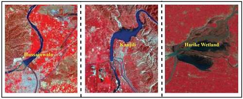
Image Pre-processing: In this study, false-color composite bands were utilized for pre-processing that helps to fulfill the necessity of the developed model. Multiple pre-processing activities such as noise reduction, atmospheric condition adjustment, and radiometric correction are performed on collected images. Furthermore, several data augmentation methods such as clipping, rotating, flipping, shifting, and transforming are used to increase the number of images to address the issue of model over-fitting that aids in the resolution of imbalanced learning (Ding et al. 2016; Ji, Wei, and Lu 2019; N. Yang et al. 2016; Perez and Wang 2017; Norouzi, Ranjbar, and Mori 2009). Moreover, the super-pixel approach is utilized to optimize the prediction performance of the proposed approach. Super-pixels are used in several computer vision and image processing methods. A super-pixel defines the group of pixels with similar characteristics. Hence, Simple Linear Iterative Clustering (SLIC) (Achanta et al. 2012) is utilized to derive the superpixels and helps to eliminate deviated pixels. In this way, the super-pixel technique in satellite images makes the borders around the object that helps in distinguishing every possible small adjacent object.

Fog Space: Water Resource Prediction

In this section, a Convolutional Restricted model-based technique is utilized for the segmentation of water bodies by analyzing RS images as represented in Figure 2. The first module is responsible to extract spatial characteristics from the RS data by utilizing the feature extraction capability of the Deep Convolutional Restricted Model (DCRM). After extracting features, the structural learning method is used in the second module to analyze the relationship between the artifacts and the environment. At last, a feature fusion layer is introduced to generate more effective image representative functions. The step-by-step process of each module is discussed below:

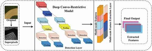
a) Deep Convo-Restricted Model: The precise identification of features toward the given object is determined as a key assessment parameter of the proposed approach in the field of RS. Therefore, Deep Convo-Restricted Model extracts spatial features from the given data by utilizing 2d-CNN and RBM techniques. The developed framework is presented in Figure 4 and explained in two layers such as Detection Layer (DL) and Visible Layer (VL).

Figure 4. The DCRM feature learning concept.

In DL, $F^k$ series of kernels are utilized to identify the features from the image and produce $D^k$ dimension matrices indicated with $N_d$ for feature extraction. A dimensional matrix with its weights and bias is indicated by $F^k$ and $b^k$, respectively. While the dimensional matrix of sub-units are expressed by $d_{ij}^k$. The variables i and j specify the ratio of convolution process. Using the pooling technique denoted with $B_{\alpha }$, the Max-pooling layers marked with m are utilized to reduce the dimension of an image. Furthermore, the VL has K number of convolutional filters and each filter has $n_f$ dimensional matrix. Convolutional kernels $F^k(k\in [i,k])$ are included to deal with the possibility of comparable characteristics of an image and shared among both DL and VL. The following formula is used to determine the cumulative probabilistic value:

(1) $m(l,d)=\frac{1}{z}exp(-e(l,d))$(1)

In this manner, the normalized parameter $s={\sum }_l{\sum }_{d}exp\left(-E(l,d)\right)$ and the DCRM energy function is computed as follows:

(2) $e(l,d)=-\sum _{k=1}^k{d}^k\odot ({\tilde{F}}^k\star l)-\sum _{k-1}^k{b}^k\sum _{ij}{d}_i{j}^k-s\sum _{ij}{l}_{ij},$(2)

Here, 2d convolution, element-wise multiplication, and flipping operations are represented by $\star$, $\odot$, and ${\tilde{C}}^k$, respectively. In this manner, the units of detecting layer DL evaluate the overall activation from smaller regions of the satellite image. To minimize the inference process in the proposed solution, the following equation is used:

(3) $\begin{array}{c}e(l,d)=-\sum _K\sum _{ij}(d_{ij}^k{({\tilde{F}}^k\star l)}_{ij}+b_k{d}_{ij}^k)-s\sum _{ij}{l}_{ij}\sum _{(ij){\beta }_{\alpha }}{l}_{ij}^k\le 1,\mathrm{\forall }k,\alpha \end{array}$(3)

Here, the fixed-shape window of the DL is represented as $B_{\alpha }$ and SGD is adopted to improve the specification of the DCRM (Z. Han et al. 2016). Moreover, the contrastive divergence (CD) approach (Hinton 2002) is employed to optimize the effectiveness of the method over the stochastic gradient descent (SGD).

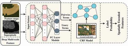
b) Structural Learning Layer (SLL): Even, CNN has the potential to obtain hierarchical features, these features are ineffective to evaluate the relationship between artifacts and spatial features. Therefore, the CRF approach is employed for detecting the SIF (Bu et al. 2016) and the procedure of accessing SIF are clearly illustrated in Figure 5. A graph method represented as g = (v,e) is introduced to manage high resolution (HR) images, where the edge $e$ is denoted as $E$ and vertex $v$ is denoted as $V$. The vertex unit refers to the image sub-segments and the border refers to the relationship between nearby unit pairs. The weight in the training data is used to generate the conditional probability distribution as follows:

(4) $x(x\parallel y,t)=\frac{1}{z(x,t)}\prod _{i\in V}{\varphi }_n(x_i,y_i)\prod _{e_{ij}\in e}{\psi }_e(x_{ij},y_i,y_j)$(4)

Figure 5. Representation of structural learning.

Here, a constructed graph model pair-wise partitioning function is expressed by $a(y,t)$. The features of a unit are specified as ${\psi }_e(x_{ije},y_i,y_j)$. Furthermore, the potentials of $f_n-F_e$ are labeled as log-linear function denoted as $e_{ij}$. An edge which is composed of $v_i$, $v_j$ and p represents the units with their respective states y = < $y_1$, $y_2$, $y_3$, … ., $y_n$ >. The training procedure has been modified as follows:

(5) $\begin{array}{c}{t}^{\ast }argmi{n}_t\lambda \parallel t{\parallel }^2-\sum _{n=1}^m(\sum _{i\in V}{t}_N^T{f}_N(x_i^n,y_i^n)+\sum _{e_{ij\in E}}{t}_E^T{f}_E(x_{ij{e}^n},y_i^n,y_i^n))+\sum _{n=1}^{m}logZ(x^n,t)\end{array}$(5)

Here, the weight of paired elements is $t=[T_N;T_E]$, where $\lambda$ is a positive L2-regularizer represented as $t=[TN;TE]$ . Additionally, the graphical model is represented as $(x_i^n,y_i^n)$. It has been analyzed that by maximizing the value can improve the chance of prediction of target class denoted as $x(y|y,t^{\ast })$.

C) Spatially Inferred Features (SIF): As per the literature review, it has been identified that the CRF is considered as one of the optimized approaches in the field of RS. Here, the integration of CRF is done for enhancing the stability of prediction. In parallel, the graphical and SIF models are applied to obtain both super-pixel and spatial features for resolving the learning limitation of spatial features. The connection in the graph is defined as $G_{\mu }=(V_{\mu },E_{\mu })$, where $\mu$ is describing as super-pixels. Moreover, $\odot (\mu )$ is used to represent the SIF model and is further calculated as follows:

(6) $\odot (\mu )=\lambda \sum _{i\in V_{\mu }}\sum _{j\in V_{\mu }}{\theta }_i{\theta }_j^{T}exp\left(-k_d\frac{d(v_i,v_j)}{{\sigma }_d}\right)$(6)

Here, the density of existence of the adjacent probability of defined vertices $i$ and $j$ is specified by $n\times n$ matrix of $odot$. Moreover, the distance between super-pixels is denoted by $d(v_i,v_j)$. Furthermore, the distance decay rate, vertice distance, and normalized parameter are represented by $k_d$, ${\sigma }_d$, and $\lambda$, respectively.

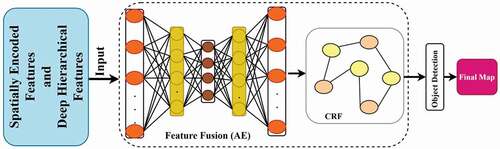
d) Multi-layered Feature Fusion (MFF): A multilayer sparse auto-encoder (SAE) is part of a multilayer feature fusion (MFF) neural network that is implemented in the proposed solution. In addition, MFF precisely obtains the hierarchical features with similar attributes from the images. Figure 6 illustrates the complete process of fusing multiple features. In the process of feature and structural learning defined as $[U_p,\odot ]\in W^{(N+nxn)}$, two different descriptors such as DHF $U_p$ and SIF $\odot$ are obtained. In addition, DSA is utilized to integrate linked data. Furthermore, the backpropagation approach is applied in the proposed solution to optimize the prediction efficiency.

Figure 6. DSA and CRF model for the extraction of hybrid features.

The sample of SAE is denoted as $X=(x_1,x_2,\dots ..,x_N{)}^T$. The hidden units $n_r$ in layer L are represented as $r_l=(r_1^L,r_2^L\dots \dots r_{nr}^L)$. The sigmoid activation functions utilized in the proposed model are further expressed as follows:

(7) $r^L=\frac{1}{1+e^{-x}}(tX+B_r)$(7)

Here, $r^L$ corresponds to the equivalent representation of the modified encoder from the X input. The value of $\sigma (z)$ will always be equal to $(1+exp(-z){)}^1,w\in R^{Nx{N}_H}$ and bias value $B_H$ will correspond to $R^{N_{H}x1}$. As a result, a $\tilde{X}$ approximation equation can be expressed as follows:

(8) $\tilde{X}=\frac{1}{1+e^{-x}}(t^T{r}^L+B_0),B_o\in R^{nx1}$(8)

To reduce the variance between X and $\tilde{X}$, $o$ is calculated as:

(9) $o=\frac{1}{n_c}\sum _{i=1}^{n_c}{∥{\tilde{X}}^i-X^i∥}^2+\beta \parallel t{\parallel }_2^2+\alpha \sum _{j=1}^{n_r}kl(p\parallel {\tilde{p}}_j)$(9)

Here, the average activation function is represented by ${\tilde{p}}_j$ of $j_{th}$ and $p$ is selected as an activation function.

Experiments

The efficacy of the proposed model is assessed on the Sentinel-2 image dataset. The system is configured as follows to carry out the experiments: Intel Core i5 2.8 GHz CPU, NVIDIA GTX-1080Ti GPU, Ubuntu 18.4 LTS Operating System, Python Programming Language. The implementation of the developed solution is evaluated and presented in distinct subsections as follows;

• Material and Methods

• Evaluation metrics

• Implementation of MDFN

• Prediction Performance

• Identification Results

• Comparative Analysis

Material and Methods

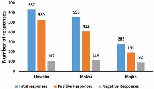
The degree of happiness index is evaluated by following two processes as follows: (i) Conducting an extensive field survey and (ii) Extraction of water resources from RS data of the targeted areas. A total number of 1476 responses have been conducted according to the three regions of Punjab such as Dowaba, Malwa, and Majha. The number of responses is divided according to the regions of Punjab. The complete detail of responses which are categorized into positive and negative responses is represented in Table 4 and illustrated in Figure 7.

Table 4. Survey collection from three regions of Punjab

Region	Total responses	Positive responses	Negative responses
Dowaba	637	530	107
Malwa	556	412	114
Majha	283	191	92

Figure 7. Number of responses according to positive and negative responses.

Evaluation Metrics

The prediction capability of the developed solution is imposed by calculating F1-score, Recall (R), Precision (P), and IoU performance measures. Moreover, the extraction of water by developed solution is justified by comparing the determined outcomes with the performance of selected state-of-the-art methodologies such as VGG, ResNet, DeepLab V3+, SegNet, NDWI, and MDFN by calculating the similar measures. Furthermore, the specified error metrics are expressed mathematically as follows:

(10) $P=\frac{TP}{TP+FP}$(10)

(11) $R=\frac{TP}{TP+FN}$(11)

(12) $F1=\frac{2\times R\times P}{R+P}$(12)

(13) $IoU=\frac{TP}{TP+FP+FN}$(13)

Implementation Of MDFN

Deep-Restrictive Model (DRM): The Deep Restrictive Model contains total $6$ convolutional layers where Ist, 2nd, and 5th layers of the architecture are responsible for executing convolutional operations. It is imperative to mention that Contrastive Divergence (CD) is utilized to fine-tune the convolutional layers. Furthermore, the 3rd, 4th, and 6th layers of the network perform the Max-pooling operation. Furthermore, the batch gradients are updated during the process of CD by leveraging the momentum from the previous gradients. Similarly, Deep Hierarchical Features (DHF) are utilized to train the Structural Learning Layer without using the method of backpropagation. In this manner, certain experiments are carried out throughout the generation of super-pixels to verify the presented solution’s efficiency and performance. Different parameters such as region size, L2 regularization ($\lambda$), and distance factor ($kd$) with the value of $0.1$ are calculated to analyze the spatial correlation among super-pixels. The sparse penalty term $\alpha$ of every hidden layer is evaluated at distant lr such as $0.2$, $0.01$, and $0.04$. Furthermore, the weight ($\beta$), activation function ($\rho$), and the LR are tuned to $0.001$, $0.05$, and $0.01$, respectively. To deal with overfitting, the proposed solution is processed with $50$ batches and $100$ epochs. The manual data division method is adopted with different ratios to evaluate the performance of the model.

Prediction Performance

In the original dataset, there are a total of 5600 images collected which are further augmented to increase the number of images to satisfy the data-hungry approach of deep learning. After executing data augmentation processes, a total of 11090 images are collected allowing for the inclusion of every imaginable real-life scenario. To evaluate the train-set and test-set efficiency, different ratios are used in dataset by utilizing the approach of manual data divisioning as shown in Table 5.

Table 5. Prediction performance evaluated on the dataset

Number of images	Data divisioning	Training samples	Validation samples	Test samples	Overall accuracy
5600	70:30	3920	1176	504	0.826
	75:25	4200	1050	350	0.852
	80:20	4480	896	224	0.899
11090	70:30	5634	2328	2327	0.919
	75:25	6238	2079	2772	0.938
	80:20	7097	1774	2218	0.958

Identification Results

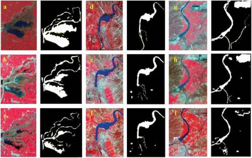
A set of 940 remote sensing images are selected from the related ground truth images to determine the prediction capability of the proposed solution. The efficacy of the developed method is measured using different ratios as presented in Table 6. The water resources from various shapes are present in the dataset that help to determine the prediction efficiency of the proposed method toward the complex pattern. The method has been considered to be accurate for the classification of water bodies in diverse locations and shapes. Furthermore, the model is capable of accurately distinguishing minor rivers and barriers such as water tunnels. To avoid the biasness in the dataset, the dataset is collected from three different locations of Punjab. The results of each location are illustrated in Figure 8.

Table 6. The derived result of P, R, F1, mIoU on different resolutions and the highest precision is highlighted

Model	Ratio	P	R	F1	mIoU
MDFN	70: 30	0.931 $\pm$ 0.016	0.912 $\pm$ 0.017	0.918 $\pm$ 0.016	0.863 $\pm$ 0.019
	75: 25	0.928 $\pm$ 0.017	0.928 $\pm$ 0.017	0.909 $\pm$ 0.015	0.863 $\pm$ 0.022
	80: 20	0.958 $\pm$ 0.013	0.878 $\pm$ 0.016	0.921 $\pm$ 0.013	0.881 $\pm$ 0.021

Table 7. The execution time of the different models

Models	Training-set		Test-set
VGG	22,960 s	382.66 m	11310 s	188.55 m
DenseNet	18,120 s	302.11 m	9120 s	152.16 m
ResNet	18,760 s	312.66 m	10239 s	170.65 m
MDFN	12,675 s	211.25 m	3389 s	56.48 m
SegNet	19,043 s	317.38 m	10589 s	176.48 m
DeepLabv3+	14555 s	242.58 m	9123 s	152.05 m

Figure 8. Comparison of different models on selected wetlands of Punjab.

Comparative Analysis

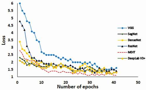
The training loss for each selected method is presented in Figure 9. In CNN, the cost function is utilized to compute the variance in the middle of the value of the ground truth of an image. Lower the loss-value means higher the accuracy value of the model. During the comparison, it has been observed that the VGG model has a higher loss value which is fairly similar to SegNet. In the early epochs, the proposed MDFN has registered higher loss. However, less loss has been observed after a certain number of epochs that indicate the stability of the proposed model. Moreover, the comparative analysis based on hyperparameters is illustrated in Table 8

Table 8. Comparison of hyperparameters

Models	Learning rate	Activation function	Batch size	Epochs
MDFN	0.01	ReLU	50	100
VGG	0.001	Sigmoid	70	100
SegNet	0.01	ReLU	40	100
ResNet	0.001	ReLU	40	100
DenseNet	0.01	Sigmoid	50	100
DeepLabv3+	0.01	ReLU	60	100

Figure 9. Training losses of different models.

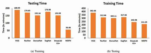
Table 7 shows the training and testing time taken by the proposed model and selected models. According to the computed results, according to the results the VGG has taken a total of 171.66 minutes of testing which is higher as compared to the others. Additionally, the proposed solution has taken less testing time with 94.37 minutes. In this manner, it can be concluded that the proposed solution has taken less testing and training time as compared to other models as presented in Table 7. Moreover, the computed outcomes are also illustrated diagrammatically in Figure 10 for easy understanding.

Figure 10. Execution time of different models.

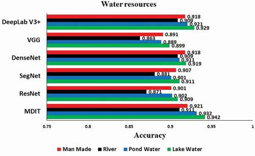
In addition, the stability of the developed solution is justified by evaluating the P, R, F1-score, and IoU. The calculated outcomes are illustrated in Table 9 and presented in Figure 11 and Figure 12. It has been observed that the proposed solution has registered the highest accuracy of $0.958$ as compared to other models. Additionally, the traditional approach NDWI model has achieved a prediction accuracy of $0.719$. Furthermore, the F1-score of the developed model achieved the accuracy of $0.928$ as compared to VGG ($0.892$), DenseNet ($0.909$), SegNet ($0.908$), DeepLabV3+ ($0.907$) and ResNet ($0.880$). Similarly, the proposed model has also achieved a higher IoU value with the value of $0.874\mathrm{\%}$ as compare to other models. Therefore, the proposed method surpasses the existing deep learning models for the segmentation of water from RS data. In addition to this, three distinct wetlands in the Punjab region were chosen between 20 August 2019 and 30 November 2019 to assess the prediction performance as presented in Figure 11.

Table 9. Comparison of different selected models with proposed solution

Metrics	MDFN	VGG	DenseNet	SegNet	ResNet	Deeplabv3+	NDWI
P	0.958$\pm$ 0.012	0.886 $\pm$ 0.014	0.926 $\pm$ 0.012	0.912 $\pm$ 0.018	0.914 $\pm$ 0.014	0.924 $\pm$ 0.012	0.719 $\pm$ 0.029
R	0.899 $\pm$ 0.016	0.877 $\pm$ 0.014	0.894 $\pm$ 0.018	0.908 $\pm$ 0.017	0.903 $\pm$ 0.013	0.897 $\pm$ 0.019	0.926 $\pm$ 0.010
F1	0.928 $\pm$ 0.013	0.892 $\pm$ 0.016	0.909 $\pm$ 0.014	0.908 $\pm$ 0.017	0.880 $\pm$ 0.017	0.907 $\pm$ 0.014	0.896 $\pm$ 0.015
IoU	0.874 $\pm$ 0.021	0.833 $\pm$ 0.023	0.868 $\pm$ 0.023	0.842 $\pm$ 0.021	0.854 $\pm$ 0.021	0.862 $\pm$ 0.021	0.758 $\pm$ 0.025

Figure 11. Water identification results of Punjab from 30 Aug 2017 to 31 Aug 2019.

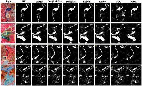
Figure 12. The prediction performance of different models on several wetlands.

Water and vegetation are represented by the blue color and red color in the original image, respectively. The lake is depicted as a pure white color in the prediction image and the dots indicates the urban area. The developed model effectively extracted the sources of water bodies from RS data and also recognized the minor ponds, rivers, and small-lakes during segmentation as presented in Figure 11. Moreover, the stability of the developed model is also better for differentiating the water and clouds. The bare land is depicted with small dots in segmentation images. Moreover, solid lines are depicted as mountain areas and dash lines marked as urban areas in images. The water bodies are isolated from the rest of the image shadows. ResNet and VGG models show various patches in the corresponding areas of the non-water area as water that defines the poor prediction performance. Meanwhile, SegNet, DeepLabV3+ and, DenseNet have also produced some false predictions. The primary water bodies are accurately recognized by the NDWI model. However, certain bare-land and dense areas are also classified as water bodies.

Survey-based Prediction Performance Analysis

The happiness index of the farmers is determined by dividing data into four different classes such as Very Happy (4), Happy (3), Neutral (2), and Not Happy (1). The degree of happiness is allocated in 4 classes where 1 defines Not Happy and 4 defines Very Happy. Furthermore, the most influential machine learning approaches such as K-Nearest Neighbors, DT, MLP, and NAÏVE BAYES is utilized to evaluate the happiness index of farmers based on the responses of the farmers. The prediction accuracy of each selected model is evaluated and presented in Table 10–12 and Table 13.

Table 10. KNN performance on four classes

No of neighbors	k = 120	k = 100	k = 70	k = 50	k = 20	k = 10
Accuracy	63.92%	64.76%	65.23%	65.12%	62.34%	62.78%

Table 11. Performance of DT on four classes

No. of depths	depth = 3	depth = 5	depth = 7	Depth = 10
Accuracy	62.67%	63.15%	64.56%	62.43%

Table 12. Performance of MLP and NAÏVE Bayes on four classes

Prediction accuracy of MLP
Hidden Layers	2	2	2	3	4
Hidden Neurons	50	100	150	100	100
Accuracy	61.43	66.23	60.22	65.25	64.45
Prediction accuracy NAÏVE BAYES
No of folds	1	2	3	4	5
Accuracy	60.43%	65.13%	59.42%	64.78%	63.34

Table 13. Comparative analysis for the calculation of happiness index by applying different models

Approaches	Original dataset	TomekLinks	SMOTE	SMOTE (SVM)	SMOTE (borderline)	ADASYN	Random Over-Sampler	SMOTETomek
KNN	68.26%	67.33%	78.61%	76.78%	76.67%	70.39%	78.43%	75.53%
Decision Tree	70.17%	61.44%	77.69%	76.40%	60.54%	60.92%	69.45%	73.57%
MLP	78.35%	79.78%	74.42%	80.19%	70.53%	67.50%	68.58%	66.48%
NAÏVE BAYES	60.53%	65.11%	64.13%	68.65%	70.78%	52.22%	58.24%	66.15%

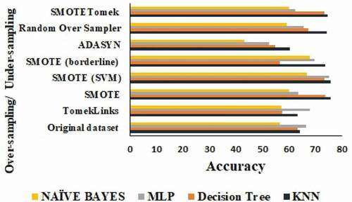
It has been observed that the accuracy of each model is improved while decreasing the number of classes. From the calculated outcome, it can be concluded that the MLP model achieved a higher accuracy of 65.25%. However, the achieved results are not satisfactory due to class imbalance in the dataset. To solve the issue of class imbalance, two major approaches are opted such as over-sampling and under-sampling. The over-sampling techniques such as SMOTE, SMOTE based on SVM, SMOTE based on borderline, RandomOverSampler, and ADASYN, and the under-sampling approaches such as TomekLinks and TomekLinks are employed. Furthermore, the calculated outcomes with respect to over-sampling and undersampling are shown below.

From the results, it has been realized that the MLP model has achieved a better accuracy of 78.35% toward the 4 classes. On the other hand, the KNN, NAÏVE BAYES, and Decision Tree registered the accuracy value of 68.26%, 60.53%, and 70.17%, respectively and illustrated in Figure 13. In this manner, a direct correlation has been observed between the availability of water and the scale of happiness of the farmers. The higher availability of water defines the higher index of happiness in farmers of that specific region. It has been observed that the Malwa and Majha regions of Punjab contain a large number of manmade water resources as compared to the Dowaba region. Therefore, a higher degree of happiness index has been calculated in the farmers of the Majha and Malwa regions. However, due to the less availability of water resources in the Dowaba region, a less degree happiness index is observed in farmers.

Figure 13. Comparative analysis of different models.

Conclusion

Advanced hardware and data processing solutions have provided the capability to analyze the frames to identify common patterns effectively. In this manner, a multi-layer data fusion approach is developed for the segmentation of water sources in a specific area by utilizing multispectral data. The purpose of this study is to analyze the degree of happiness index in the farmers of different regions of state Punjab toward the availability of water at their specific location. The maximum prediction accuracy is achieved by integrating DSA that evaluates spatial features from the data. Furthermore, the DRCM-assisted unsupervised learning solution is also integrated with the proposed solution for the extraction of complex characteristics from the labeled data. The determined outcomes define the efficacy of the developed solution for the prediction of the source of water from different RS samples by registering the higher rate of F1 $(0.928)$, IoU $(0.874)$, Recall $(0.899)$, and Precision $(0.958)$. Moreover, the higher accuracy in the performance measures achieved by the proposed solution has outperformed the selected models concerning the prediction of the sources of water from Rs images. Furthermore, the conducted survey defines the higher correlation between the degree of happiness in farmers toward the availability of water resources in that specific location. In this manner, the proposed solution can be considered to analyze the degree of happiness of the individuals related to the other social aspects such as urban development, food security, and many others.

Disclosure statement

No potential conflict of interest was reported by the authors.

Notes

1. Source: https://scihub.copernicus.eu/

References

- Achanta, R., A. Shaji, K. Smith, A. Lucchi, P. Fua, and S. Süsstrunk. 2012. SLIC superpixels compared to state-of-the-art superpixel methods. IEEE Transactions on Pattern Analysis and Machine Intelligence 34 (11):2274–82. doi:https://doi.org/10.1109/TPAMI.2012.120.
- Afaq, Y., and A. Manocha. 2021a. Fog-Inspired water resource analysis in urban areas from satellite images. Ecological Informatics 64:101385. doi:https://doi.org/10.1016/j.ecoinf.2021.101385.
- Afaq, Y., and A. Manocha. 2021b. Analysis on change detection techniques for remote sensing applications: A review. Ecological Informatics 63:101310. doi:https://doi.org/10.1016/j.ecoinf.2021.101310.
- Bu, S., P. Han, Z. Liu, and J. Han. 2016. Scene parsing using inference embedded deep networks. Pattern Recognition 59:188–98. doi:https://doi.org/10.1016/j.patcog.2016.01.027.
- Chen, Y., R. Fan, X. Yang, J. Wang, and A. Latif. 2018. Extraction of urban water bodies from high-resolution remote-sensing imagery using deep learning. Water 10 (5):585. doi:https://doi.org/10.3390/w10050585.
- Chopra, R., V. K. Verma, and P. K. Sharma. 2001. Mapping, monitoring and conservation of Harike Wetland ecosystem, Punjab, India, through remote sensing. International Journal of Remote Sensing 22 (1):89–98. doi:https://doi.org/10.1080/014311601750038866.
- Ding, J., B. Chen, H. Liu, and M. Huang. 2016. Convolutional neural network with data augmentation for SAR target recognition. IEEE Geoscience and Remote Sensing Letters 13 (3):364–68.
- Du, N., H. Ottens, and R. Sliuzas. 2010. Spatial impact of urban expansion on surface water bodies—A case study of Wuhan, China. Landscape and Urban Planning 94 (3–4):175–85. doi:https://doi.org/10.1016/j.landurbplan.2009.10.002.
- Du, Y., Y. Zhang, F. Ling, Q. Wang, W. Li, and X. Li. 2016. Water bodies’ mapping from sentinel-2 imagery with modified normalized difference water index at 10-m spatial resolution produced by sharpening the SWIR band. Remote Sensing 8 (4):354. doi:https://doi.org/10.3390/rs8040354.
- Famiglietti, J. S., and M. Rodell. 2013. Water in the balance. Science 340 (6138):1300–01. doi:https://doi.org/10.1126/science.1236460.
- Fang, W., C. Wang, X. Chen, W. Wan, H. Li, S. Zhu, Y. Fang, B. Liu, and Y. Hong. 2019. Recognizing global reservoirs from Landsat 8 images: A deep learning approach. IEEE Journal of Selected Topics in Applied Earth Observations and Remote Sensing 12 (9):3168–77. doi:https://doi.org/10.1109/JSTARS.2019.2929601.
- Feng, L., C. Hu, X. Han, X. Chen, and L. Qi. 2015. Long-Term distribution patterns of chlorophyll-a concentration in China’s largest freshwater lake: MERIS full-resolution observations with a practical approach. Remote Sensing 7 (1):275–99. doi:https://doi.org/10.3390/rs70100275.
- Feyisa, G. L., H. Meilby, R. Fensholt, and S. R. Proud. 2014. Automated water extraction index: A new technique for surface water mapping using Landsat imagery. Remote Sensing of Environment 140:23–35. doi:https://doi.org/10.1016/j.rse.2013.08.029.
- Fisher, A., N. Flood, and T. Danaher. 2016. Comparing Landsat water index methods for automated water classification in Eastern Australia. Remote Sensing of Environment 175:167–82. doi:https://doi.org/10.1016/j.rse.2015.12.055.
- Geng, Z., N. Chen, Y. Han, and B. Ma. 2020. An improved intelligent early warning method based on MWSPCA and its application in complex chemical processes. The Canadian Journal of Chemical Engineering 98 (6):1307–18. doi:https://doi.org/10.1002/cjce.23674.
- Han, Y., G. Chen, Z. Li, Z. Geng, F. Li, and B. Ma. 2020. An asymmetric knowledge representation learning in manifold space. Information Sciences 531:1–12. doi:https://doi.org/10.1016/j.ins.2020.04.036.
- Han, Z., Z. Liu, J. Han, C.-M. Vong, S. Bu, and X. Li. 2016. Unsupervised 3D local feature learning by circle convolutional restricted Boltzmann machine. IEEE Transactions on Image Processing 25 (11):5331–44. doi:https://doi.org/10.1109/TIP.2016.2605920.
- Hinton, G. E. 2002. Training products of experts by minimizing contrastive divergence. Neural Computation 14 (8):1771–800. doi:https://doi.org/10.1162/089976602760128018.
- Huang, C., Y. Chen, J. Wu, L. Li, and R. Liu. 2015. An evaluation of Suomi NPP-VIIRS data for surface water detection. Remote Sensing Letters 6 (2):155–64. doi:https://doi.org/10.1080/2150704X.2015.1017664.
- Isikdogan, F., A. C. Bovik, and P. Passalacqua. 2017. Surface water mapping by deep learning. IEEE Journal of Selected Topics in Applied Earth Observations and Remote Sensing 10 (11):4909–18. doi:https://doi.org/10.1109/JSTARS.2017.2735443.
- Isikdogan, L. F., A. Bovik, and P. Passalacqua. 2019. Seeing through the clouds with deepwatermap. IEEE Geoscience and Remote Sensing Letters 17 (10):1662–66. doi:https://doi.org/10.1109/LGRS.2019.2953261.
- Ji, S., S. Wei, and M. Lu. 2019. A scale robust convolutional neural network for automatic building extraction from aerial and satellite imagery. International Journal of Remote Sensing 40 (9):3308–22. doi:https://doi.org/10.1080/01431161.2018.1528024.
- Kang, L., S. Zhang, Y. Ding, and X. He. 2016. Extraction and preference ordering of multireservoir water supply rules in dry years. Water 8 (1):28. doi:https://doi.org/10.3390/w8010028.
- Katz, D. 2016. Undermining demand management with supply management: Moral hazard in Israeli water policies. Water 8 (4):159. doi:https://doi.org/10.3390/w8040159.
- Kumar, G., and K. Kumari. 2020. Mapping and monitoring the selected Wetlands of Punjab, India, using geospatial techniques. Journal of the Indian Society of Remote Sensing 9 48 (4):615–25. https://doi.org/https://doi.org/10.1007/s12524-020-01104-9.
- Ladhar, S. S. 2002. Status of ecological health of Wetlands in Punjab, India. Aquatic Ecosystem Health & Management 5 (4):457–65. doi:https://doi.org/10.1080/14634980290002002.
- Lee, H., R. Grosse, R. Ranganath, and A. Y. Ng 2009, June. Convolutional deep belief networks for scalable unsupervised learning of hierarchical representations. Proceedings of the 26th annual international conference on machine learning, 609–16, USA.
- Li, L., Y. Chen, T. Xu, R. Liu, K. Shi, and C. Huang. 2015. Super-Resolution mapping of wetland inundation from remote sensing imagery based on integration of back-propagation neural network and genetic algorithm. Remote Sensing of Environment 164:142–54. doi:https://doi.org/10.1016/j.rse.2015.04.009.
- Li, R., W. Liu, L. Yang, S. Sun, W. Hu, F. Zhang, and W. Li. 2018. DeepUNet: A deep fully convolutional network for pixel-level sea-land segmentation. IEEE Journal of Selected Topics in Applied Earth Observations and Remote Sensing 11 (11):3954–62. doi:https://doi.org/10.1109/JSTARS.2018.2833382.
- Ma, L., Y. Liu, X. Zhang, Y. Ye, G. Yin, and B. A. Johnson. 2019. Deep learning in remote sensing applications: A meta-analysis and review. ISPRS Journal of Photogrammetry and Remote Sensing 152:166–77. doi:https://doi.org/10.1016/j.isprsjprs.2019.04.015.
- Manocha, A., G. Kumar, M. Bhatia, and A. Sharma. 2020. Video-assisted smart health monitoring for affliction determination based on fog analytics. Journal of Biomedical Informatics 109:103513. 109. doi:https://doi.org/10.1016/j.jbi.2020.103513.
- McFeeters, S. K. 1996. The use of the Normalized Difference Water Index (NDWI) in the delineation of open water features. International Journal of Remote Sensing 17 (7):1425–32. doi:https://doi.org/10.1080/01431169608948714.
- Norouzi, M., M. Ranjbar, and G. Mori. 2009. Stacks of convolutional restricted Boltzmann machines for shift-invariant feature learning. 2009 IEEE Conference on Computer Vision and Pattern Recognition, 2735–42, Miami, FL. IEEE.
- Perez, L., and J. Wang. 2017. The effectiveness of data augmentation in image classification using deep learning. ArXiv Preprint ArXiv:1712.04621.
- Shuster, W. D., J. Bonta, H. Thurston, E. Warnemuende, and D. R. Smith. 2005. Impacts of impervious surface on watershed hydrology: A review. Urban Water Journal 2 (4):263–75. doi:https://doi.org/10.1080/15730620500386529.
- Tambe, R. G., S. N. Talbar, and S. S. Chavan. 2021. Deep multi-feature learning architecture for water body segmentation from satellite images. Journal of Visual Communication and Image Representation 77:103141. doi:https://doi.org/10.1016/j.jvcir.2021.103141.
- Weinstein, S., and P. Ebert. 1971. Data transmission by frequency-division multiplexing using the discrete Fourier transform. IEEE Transactions on Communication Technology 19 (5):628–34. doi:https://doi.org/10.1109/TCOM.1971.1090705.
- Wu, Y., L. Mengru, L. Guo, H. Zheng, and H. Zhang. 2019. Investigating water variation of lakes in Tibetan Plateau using remote sensed data over the past 20 years. IEEE Journal of Selected Topics in Applied Earth Observations and Remote Sensing 12 (7):2557–64. doi:https://doi.org/10.1109/JSTARS.2019.2898259.
- Xie, C., X. Huang, L. Wang, X. Fang, and W. Liao. 2018. Spatiotemporal change patterns of urban lakes in China’s major cities between 1990 and 2015. International Journal of Digital Earth 11 (11):1085–102. doi:https://doi.org/10.1080/17538947.2017.1374476.
- Xu, H. 2006. Modification of Normalised Difference Water Index (NDWI) to enhance open water features in remotely sensed imagery. International Journal of Remote Sensing 27 (14):3025–33. doi:https://doi.org/10.1080/01431160600589179.
- Yan, Y., H. Zhao, C. Chen, L. Zou, X. Liu, C. Chai, C. Wang, J. Shi, and S. Chen. 2018. Comparison of multiple bioactive constituents in different parts of eucommia ulmoides based on UFLC-QTRAP-MS/MS combined with PCA. Molecules 23 (3):643. doi:https://doi.org/10.3390/molecules23030643.
- Yang, N., H. Tang, H. Sun, and X. Yang. 2016. Dropband: A convolutional neural network with data augmentation for scene classification of VHR satellite images.
- Yang, X., S. Zhao, X. Qin, N. Zhao, and L. Liang. 2017. Mapping of urban surface water bodies from sentinel-2 MSI imagery at 10 m resolution via NDWI-Based image sharpening. Remote Sensing 9 (6):596. doi:https://doi.org/10.3390/rs9060596.
- Yu, L., Z. Wang, S. Tian, F. Ye, J. Ding, and J. Kong. 2017. Convolutional neural networks for water body extraction from Landsat imagery. International Journal of Computational Intelligence and Applications 16 (1):1750001. doi:https://doi.org/10.1142/S1469026817500018.
- Yurtkulu, S. C., Y. H. Sahin, and G. Unal. 2019. Semantic segmentation with extended DeepLabv3 architecture. 2019 27th Signal Processing and Communications Applications Conference (SIU), 1–4., Sivas, Turkey, IEEE.
- Zhang, L., G.-S. Xia, T. Wu, L. Lin, and X. C. Tai. 2016. Deep learning for remote sensing image understanding. Hindawi.
- Zhou, Y., J. Luo, Z. Shen, X. Hu, and H. Yang. 2014. Multiscale water body extraction in urban environments from satellite images. IEEE Journal of Selected Topics in Applied Earth Observations and Remote Sensing 7 (10):4301–12. doi:https://doi.org/10.1109/JSTARS.2014.2360436.
- Zhu, X. X., D. Tuia, L. Mou, G.-S. Xia, L. Zhang, F. Xu, and F. Fraundorfer. 2017. Deep learning in remote sensing: A comprehensive review and list of resources. IEEE Geoscience and Remote Sensing Magazine 5 (4):8–36. doi:https://doi.org/10.1109/MGRS.2017.2762307.