A Credit Risk Model with Small Sample Data Based on G-XGBoost

ABSTRACT

Currently existing credit risk models, e.g., Scoring Card and Extreme Gradient Boosting (XGBoost), usually have requirements for the capacity of modeling samples. The small sample size may result in the adverse outcomes for the trained models which may neither achieve the expected accuracy nor distinguish risks well. On the other hand, data acquisition can be difficult and restricted due to data protection regulations. In view of the above dilemma, this paper applies Generative Adversarial Nets (GAN) to the construction of small and micro enterprises (SMEs) credit risk model, and proposes a novel training method, namely G-XGBoost, based on the XGBoost model. A few batches of real data are selected to train GAN. When the generative network reaches Nash equilibrium, the network is used to generate pseudo data with the same distribution. The pseudo data is then combined with real data to form an amplified sample set. The amplified sample set is used to train XGBoost for credit risk prediction. The feasibility and advantages of the G-XGBoost model are demonstrated by comparing with the XGBoost model.

Introduction

In recent years, internet finance has been developing rapidly in the world, particularly in the developing countries like China. However, due to the imperfection of the existing credit system and the outdated technology, the internet financial industry is facing great challenges (Zheng 2014). It is widely recognized that the key of Internet finance lies in risk management, and the core of risk management lies in data as the management aims to solve the risks and uncertainties in investment decisions (Cheng 2014).

How to deal with credit risk? The first choice of traditional financial institutions is the credit score card model (Wiginton 1980). The basic tool is logistic regression. Analysts use a large amount of historical data to describe user’s income level, payment ability, credit status and other indicators, and then divide the indicators into several levels. Different levels of indicators are assigned with different weights, and finally user’s credit scores are calculated (Mamdouh 2011). With the development of Internet finance, the application of machine learning methods (Nedellec et al. 1994; Boz et al. 2018; Shukla and Nanda 2019), e.g., Decision Tree (Kruppa et al. 2013), Neural Network (Luo, Wu, and Wu 2016), Monte Carlo (Andrade and Sicsú 2008) and Extreme Gradient Boosting (XGBoost) (Liu, Huang, and Xie 2019; Qiu 2019), in the financial credit risk starts to flourish. These methods have their own advantages and disadvantages (Zhang et al. 2007; Tran, Duong, and Ho 2016; Wang et al. 2017; Li Y. 2019b; Hindistan et al. 2019; Wang et al. 2019a).

Logistic regression does not assume any probability distribution, nor does it require equal covariance. However, when the sample points are completely separated, the maximum likelihood estimation of the model parameters may not exist. Thereby the stability and validity of the model may have problems, leading to the instability of the final result. Decision tree seems easier to understand intuitively. However, the combinatorial explosion often occurs with the growth of the decision tree, which leads to the over-complexity, difficulty to understand, and a tendency toward an overfitted model. Machine learning does not impose restrictions on data distribution, but it has problems such as interpretability, large training sample set and low training efficiency. At present, XGBoost is used as the main machine learning method in the construction and analysis of the credit risk model in Internet finance companies.

The construction of credit risk model needs not only enough variables for representing the model dynamics, but also a sufficient amount of sample data for training the model. In general, the data size should not be too small, nor too large (Feng et al. 2019; Li C.Y. 2019a). However, due to the difficulty of data acquisition and high cost of data, it is difficult to satisfy the optimal data size for modeling in reality. The optimal data size needed to establish a model with the optimal prediction accuracy and robust performance remains an open question as there is no quantitative analysis, except for some empirical estimations, at present.

To ensure the stability of the model, it is generally required that the number of good and bad samples should be at least 20 times more than the number of independent variables (Jin 2003). In practice, we often face the facts of samples either less than required or of extreme imbalance problem. These cases, for certain, will compromise the accuracy and stability of the model. For example, when the number of users is relatively small in the early stage of a product, and meanwhile the credit samples of small and micro enterprises (SMEs) are very small, the bad ratio is very low, which puts forward the need for how to use the small sample data to build the credit risk model (Chi 2014; Li et al. 2016; Ma 2019).

This paper proposes a solution to tackling the aforementioned problems by using Generative Adversarial Nets (GAN) for alleviating issues associated with small samples. At the same time, XGBoost is selected as the prediction algorithm, which is one of the most widely used model in the financial risk control field at present. By combining GAN and XGBoost (G-XGBoost), this work explores the application of GAN in financial credit risk of SMEs. A comparative analysis on the effectiveness and performance of the G-XGBoost algorithm is conducted to validate the method.

The rest of the paper is organized as follows. Section II introduces the GAN, XGBoost algorithms, and the model evaluation index of KS and AUC. Section III presents the model and related influencing variable. Section IV describes the work process and discusses the experiment results. Section V concludes the work and provides possible future directions.

Algorithms and Evaluation

Generative Adversarial Nets

GAN is a deep learning model, which was first proposed by Goodfellow et al. (2014). The optimization process of GAN is a minimax two-player game problem, whose optimization goal is to achieve Nash equilibrium (Ratliff, Burden, and Sastry 2016). During the past years, GAN has been used in computer vision (Antoniou, Storkey, and Edwards 2018; Lee and Cho 2020; Mehta et al. 2019; Mirza and Osindero 2014; Radford, Metz, and Chintala 2016; Wang et al. 2018, 2019b). At the same time, some studies have applied GAN to data amplification, effectively solving the problem of insufficient data, such as trajectory prediction, electric power, medical and other industries (Chen et al. 2018; Frid-Adar et al. 2018; Gupta et al. 2018; Rahbar et al. 2019; Wiese et al. 2020).

The GAN is shown in Figure 1, which consists of two parts: the generator G and the discriminator D. Generator G is used to obtain the distribution of data, and discriminator D is used to estimate the probability of data from training samples or generator G. G is trained to maximize D’s chances of making mistakes. The model is similar to a two-player game, and there is a unique solution existing in the functional solution space of G and D. With the distribution of training data obtained by G, the probability of D output gradually approaches 1/2. When G and D are defined as multi-layer perceptrons, the system is trained by the back propagation of errors. In the process of training and generating samples, no Markov chain or approximate inference network is needed.

Figure 1. The basic structure of GAN.

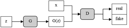
Generator G: a generative net, generating pseudo data $G\left(z\right)$ by receiving predefined noise z;

Discriminator D: a discriminative net, determining the probability $D\left(x\right)$ of whether the output data is true data or not by receiving the input sample data x.

The purpose of the discriminator D is to distinguish the true and false data. The closer to 1 the function output of $D\left(x\right)$ of the original sample data x is, the better, and the closer to 0 of $D\left(G\left(z\right)\right)$ is, the better. The purpose of the generator G is to make the pseudo data $G\left(z\right)$ generated by the model G to cheat the discriminator D as much as possible, that is, the bigger the $D\left(G\left(z\right)\right)$ the better (Gao and Jiang 2019). Therefore, the training of D and G becomes a minimax problem:

(1) $\underset{G}{min}\underset{D}{max}V\left(D,G\right)=E_{x\text{~}{p}_{data}\left(x\right)}\left[logD\left(x\right)\right]+E_{z\text{~}{p}_z\left(z\right)}\left[log\left(1-D\left(G\left(z\right)\right)\right)\right]$(1)

Where, $p_{data}\left(x\right)$ is the distribution of real data, $p_z\left(z\right)$ is the distribution of pseudo data. The cost function corresponding to generator G and discriminator D are:

(2) $\underset{G}{min}V\left(D,G\right)=-E_{z\text{~}{p}_z\left(z\right)}\left[log\left(1-D\left(G\left(z\right)\right)\right)\right]$(2)

(3) $\underset{D}{max}V\left(D,G\right)=-E_{x\text{~}{p}_{data}\left(x\right)}\left[logD\left(x\right)\right]-E_{z\text{~}{p}_z\left(z\right)}\left[log\left(1-D\left(G\left(z\right)\right)\right)\right]$(3)

Extreme Gradient Boosting

XGBoost is a general Tree Boosting algorithm, which is an improvement on Gradient Boosting Decision Tree (GBDT) (Friedman 2001), proposed by Chen and Guestrin in 2016. The basic idea of XGBoost is to split features to grow trees. A tree is added in an iteration of computing to learn with a new function to fit the residual predicted in the last iteration.

For a given data set with n examples and m features $D=\left\{\left(x_i,y_i\right)\right\}\left(\left|D\right|=n,x_i\in R^m,y_i\in R\right)$, a tree ensemble model uses K additive functions to predict the output.

(4) $\widehat{y_i}=\varphi \left(X_i\right)=\sum _{k=1}^K{f}_k\left(X_i\right),f_k\in F$(4)

Where, $F=\left\{f\left(x\right)={\omega }_{q\left(x\right)}\right\}\left(q:R^m\to T,\omega \in R^T\right)$ is the space of regression trees, q is the structure of each tree that maps an example to the corresponding leaf index, T is the number of leaves in the tree, and each $f_k$ corresponds to an independent tree structure q and leaf weights $\omega$. Unlike decision trees, each regression tree contains a continuous score on each of the leaf, ${\omega }_i$ is the score on i-th leaf. Its objective function is:

(5) $L\left(\varphi \right)=\sum _{i}l\left(\widehat{y_i},y_i\right)+\sum _k\mathrm{\Omega }\left(f_k\right)$(5)

Where, $\mathrm{\Omega }\left(f\right)=\gamma T+\frac{1}{2}\lambda {\left|\left|\omega \right|\right|}^2$, L is differentiable convex loss function that represents the error between the predicted result $\widehat{y_i}$ and the actual result $y_i$. At the same time, in order to avoid model overfitting, the regular term $\mathrm{\Omega }$ is added.

Compared to GBDT, XGBoost can automatically utilize multithreading of CPU for parallelism, and improve the accuracy of algorithm. In addition, XGBoost supports custom cost functions, as the function can be first-order and second-order derivative. XGBoost adds regular terms to the cost function to control the complexity of the model. The regular term contains the number of leaf nodes of the tree and the sum of the squares of L2 modules of the output fractions of each leaf node. The regular term reduces the variance of the model, makes the learned model simpler and prevents over fitting.

Model Evaluation Index

The common evaluation indexes in the financial credit risk include confusion matrix, Kolmogorov-Smirnov (KS) value, Area Under Curve (AUC) value, etc. (Mamdouh 2011). This paper selects KS and AUC to evaluate the model.

As shown in Table 1, TP represents the samples that are correctly judged as good customers, TP+FN represents all samples that are actually good customers. FP represents the samples that are wrongly judged as good customer, FP+TN represents all samples that are actually bad customers. TPR = TP/(TP+FN), is called hit rate or sensitivity, which means the percentage of all samples that are actually good customers, that are correctly judged as good customers. FPR = FP/(FP+TN), is called false positive rate, which means the percentage of all samples that are actually bad customers, that are wrongly judged as good customers.

Table 1. The confusion matrix

	Test outcome-Positive	Test outcome- Negative	Total
Condition-Positive	True Positive (TP)	False Negative (FN)	TP+FN
Condition-Negative	False Positive (FP)	True Negative (TN)	FP+TN
Total	TP+FP	FN+TN	TP+FP+FN+TN

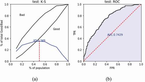
The KS curve is shown in Figure 2(a). Divide the population into n (usually 10) equal parts and arrange them in descending order according to the default probability, calculate the cumulative distribution of default and normal percentage in each equal part, draw the difference between them, and then get the KS curve. The maximum value in the KS curve is called the KS value, and is between 0 and 1. The higher the KS value, the stronger the ranking ability of the model, the stronger the prediction ability. When random sampling, the KS value is 0. When optimal classification, the KS value is 1.

Figure 2. Model evaluation – KS diagram and ROC diagram.

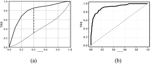
The Receiver Operating Characteristic (ROC) curve is based on the confusion matrix. FPR is defined as the X-axis and TPR as the Y-axis, as shown in Figure 2(b). Given a threshold, a coordinate point (x = FPR, y = TPR) can be calculated from the real and predicted values of all samples. The ROC curve is drawn by changing the threshold from 0 to the maximum set of coordinate points. The area under the ROC curve is called AUC value, which is also an indicator of model, indicating the probability that the predicted positive case will be ranked ahead of the negative case. The higher the AUC value, the better the prediction effect of the model.

Model and Variable

In this paper, GAN is used for data generation and XGBoost is used for prediction, so as to realize the mapping relationship between many influencing factors and the final result. The detailed process is shown in Figure 3.

Figure 3. Flow chart of model construction.

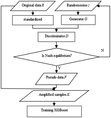
Because there are many factors influencing the credit risk of SMEs, and the dimensions of different factors are remarkably different, direct use of the data is difficult. Therefore, in the experiment, the original data is normalized into the range of [−1,1]. Transformation formula between each group of influencing factors.

(6) $x_i=\frac{x_i-min\left(x\right)}{max\left(x\right)-min\left(x\right)}\times 2-1$(6)

The GAN is trained by the normalized data, using random noise and real sample data, in which the game between generator G and discriminator D continues, until they reach the Nash equilibrium. Finally, the powerful networks G and D are obtained which can simulate the original data.

The generator G generates pseudo data $G\left(z\right)$ by receiving random noise z. Assuming that the distribution of training samples $p\left(x\right)$ is known, then new samples can be randomly sampled from the distribution. The generator is to get the relationship between noise z and training sample x in training. In the experiment, the random noise obeys the Gaussian distribution $N\left(0,1\right)$.

The discriminator D, by receiving input x, determines the probability $D\left(\mathrm{x}\right)$ of whether the data is true or $G\left(\mathrm{z}\right)$. Through the mutual game and training of G and D, the performance of nets is improved, and finally reaches the Nash equilibrium state.

In the GAN, we can update the discriminator by ascending its stochastic gradient, and update the generator by descending its stochastic gradient. The maximum number of iterations is T. The number of training steps k is a hyper parameter, k = Round (N/batch), where Ronud (*) is the rounding function, N is the sample size, and batch is the number of samples taken each time.

Select batch of m samples $\left\{z_1,z_2,\cdots ,z_m\right\}$ from pseudo data $p_z\left(z\right)$ and batch of m samples $\left\{x_1,x_2,\cdots ,x_m\right\}$ from real data $p_{data}\left(\mathrm{x}\right)$. Then their cost functions were calculated using Eq. 3(3) $\underset{D}{max}V\left(D,G\right)=-E_{x\text{~}{p}_{data}\left(x\right)}\left[logD\left(x\right)\right]-E_{z\text{~}{p}_z\left(z\right)}\left[log\left(1-D\left(G\left(z\right)\right)\right)\right]$(3) to update the discriminator by ascending its stochastic gradient (Goodfellow et al. 2014).

(7) ${\mathrm{\nabla }}_{{\theta }_d}1\text{overm}\sum _{i=1}^m\left[logD\left(x_i\right)+log\left(1-D\left(G\left(z_i\right)\right)\right)\right]$(7)

After the discriminator was updated with k times of training, select batch of m samples $\left\{z_1,z_2,\cdots ,z_m\right\}$ from $p_z\left(z\right)$. Then their cost functions were calculated using Eq.2(2) $\underset{G}{min}V\left(D,G\right)=-E_{z\text{~}{p}_z\left(z\right)}\left[log\left(1-D\left(G\left(z\right)\right)\right)\right]$(2) to update the generator by descending its stochastic gradient:

(8) ${\mathrm{\nabla }}_{{\theta }_g}1\text{overm}\sum _{i=1}^{m}log\left(1-D\left(G\left(z_i\right)\right)\right)$(8)

Let’s assume that we have a set of vectors data, and $p_{data}\left(x\right)$ is the distribution of real data. During the training process, $p_z\left(z\right)$ gradually converges to $p_{data}\left(x\right)$. The proposition is shown as follows:

Proposition 1: For G fixed, the optimal discriminator D is:

(9) $D^{\ast }\left(x\right)=\frac{p_{data}\left(x\right)}{p_{data}\left(x\right)+p_z\left(x\right)}$(9)

Proposition 2: If G and D have enough capacity, and at each step of algorithm the discriminator D is allowed to reach its optimum given G, and $p_z\left(x\right)$ is updated so as to improve the criterion:

(10) $E_{x\text{~}{p}_{data}\left(x\right)}\left[log{D}_G^{\ast }\left(x\right)\right]+E_{z\text{~}{p}_z\left(x\right)}\left[log\left(1-D_G^{\ast }\left(x\right)\right)\right]$(10)

If the formula reaches the optimal value, then $D^{\ast }\left(x\right)=1/2$, that is, $p_z\left(x\right)=p_{data}\left(\mathrm{x}\right)$.

According to Proposition1 and 2, after the whole model reaches Nash equilibrium, the generator has obtained a good estimated distribution of the original data distribution, $p_z\left(z\right)$=$p_{data}\left(\mathrm{x}\right)$.

After training the network, pseudo data F is generated by the trained generator, and the amplified sample K is composed of the original sample data R and the pseudo data F. Compared with the original data R, the distribution of the amplified samples K is essentially the same, while the amount of data is significantly improved. Now, XGBoost can be trained with the amplified sample K for risk prediction.

This paper takes the credit risk model of SME as an example. Compared with individual credit risk, SME have a smaller amount of customer data and a lower rate of bad customers. However, once default occurs, the risk of loss is high. Based on the actual situation, the following variables are selected as influencing factors, for instance, the financial information of the enterprise and the information of the enterprise legal person, as shown in Table 2.

Table 2. The influencing variable

Category	Variable
Enterprise basic information	industry, number of employees, length of existence, industrial and commercial registration status, registered capital, etc
Enterprise equity information	legal person, changes in shareholders, borrowing enterprise equity ratio, etc
Enterprise judicial information	litigation and bad records, such as enterprise breach of faith, execution, court notice, judgment documents, etc
Enterprise related party information	related party quantity, related party operation and related lawsuit, etc
Enterprise business information	financial information, such as enterprise quick ratio, operating margin, total assets turnover, accounts receivable turnover, return on total assets, etc
Enterprise credit information	credit history, current liabilities, contingent liabilities, credit demand, default and overdue situation, etc
Legal person basic information	age, education, sex, marital status, etc
Legal person assets information	deposits and other financial products, etc
Legal person debt information	loan type, loan date, loan amount, etc
Legal person judicial information	litigation and bad record, etc
Legal person credit information	credit history, current liabilities, contingent liabilities, credit demand, default and overdue, etc
Macroeconomic information	GDP, CPI, PPI, etc

Experiment and Analysis

A set of 2,000 original customer samples containing 128 variables is collected, of which 585 are bad samples (y = 1), and the rest are good samples (y = 0). In the experiment, 500 samples are randomly selected as the verification set, and the bad ratio in the verification set is same with the original data. Then, the remaining 1,500 samples are used as the training set for XGBoost and G-XGBoost, in which the GAN in the G-XGBoost model was trained with the good samples and the bad samples respectively.

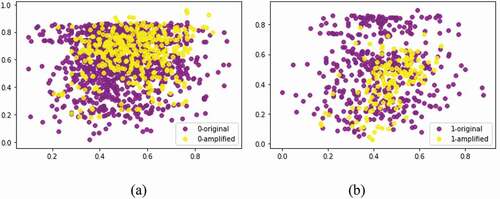
After training the network, pseudo data is generated by the trained generator, and the amplified sample is composed of the original sample data and the pseudo data. Compared with the original data, the distribution of the amplified samples is essentially the same, while the amount of data is significantly improved, as shown in Figure 4.

Figure 4. The distribution of the amplified data is consistent with the original data.

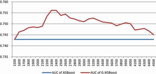
In order to explore the influence of the number of amplified samples on the training results, each time the set of samples is amplified by 100 more generated samples with the same bad ratio of the original data. For the same amplified threshold, randomly generate five different pseudo data set, combine with the original data form different amplified data, training of the G-XGBoost model using the amplified data, calculate the average of KS and AUC, and the change curve of KS and AUC with the increase of the sample size is obtained, as shown in Figure 5 and Figure 6.

Figure 5. KS under different amplified sample thresholds.

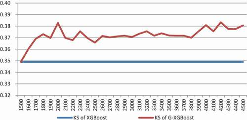
Figure 6. AUC under different amplified sample thresholds.

As shown in Figure 5, the x-axis represents the number of the amplified sample (the original sample size is 1500, increasing by 100 pseudo data each time), and the y-axis represents the average of KS. When the amplified sample size is 1,500 to 2,000, the KS value shows an obvious upward trend with the increase of the sample size. From 2,000 to 3,000, with the increase of samples, the KS value fluctuated slightly, but it was still significantly better than the original, non-amplified sample. Then the KS value gradually increased and stabilized. In general, the G-XGBoost model is better than the XGBoost model trained by the original samples in terms of the KS value.

As shown in Figure 6, the x-axis represents the number of the amplified sample (the original sample size is 1500, increasing by 100 pseudo data each time), and the y-axis represents the average of AUC. When the amplified sample size is 1,500 to 2,300, the AUC value increases and reaches the maximum value when the sample size is about 2,300. Then, the AUC value shows a small fluctuation, with the overall downward trend.

In combination with Figure 5 and Figure 6, increasing the number of samples in the early stage will improve the model effect. After reaching a certain threshold, the model effect will be optimal, as described in the section I, there is an optimal sample size that optimizes the model. After that, the increase of sample size will have limited or even negative impact on the model effect. This phenomenon might be attributed to the deviations of the GAN generated samples from the distribution of real samples. In addition, it may be error-prone when the amount of amplified data is too large. The addition of many deviated, and therefore erroneous samples to the training set will have accumulative effects accounting for the inaccuracy of the model with declined performance.

Generally speaking, the G-XGBoost model is better than the current mainstream credit risk XGBoost model, with a requirement of sample size selection.

In order to further verify the effectiveness of the G-XGBoost model, cross validation is conducted in the experiment. The original samples are split randomly into four groups, one different group (500 samples) is selected as the verification set, and the other three groups as training sets to train XGBoost and G-XGBoost, respectively. In addition, in the G-XGBoost model, one more training group composed of 500 GAN generated samples is used. This process is repeated for four times. The KS and AUC values are compared on the verification set, as shown in Table 3.

Table 3. The KS and AUC value of different model

	KS of XGBoost	AUC of XGBoost	KS of G-XGBoost	AUC of G-XGBoost
Group1	0.3490	0.7429	0.3968	0.7499
Group2	0.3841	0.7508	0.4042	0.7491
Group3	0.3623	0.7534	0.3903	0.7564
Group4	0.3618	0.7342	0.3664	0.7354
Average	0.3643	0.7453	0.3894	0.7477

Table 3 shows the KS value of G-XGBoost (+500 generated samples) is significantly higher than that of XGBoost either from single group or the average, indicating that the G-XGBoost model has indeed improved the ability of risk discrimination. Table 3 shows the two models are very close in prediction accuracy, with the G-XGBoost (+500 generated samples) slightly more accurate than XGBoost except for the second group.

For clarity, a more detailed comparison between the two models by using Group 1 as shown in Tables 3 and 4 are made.

Table 4. The statistics of Model 1 validation sets

Level	Predicted values	Good	Bad	Good%	Bad%	Bad ratio	KS
1	>0.581	17	33	4.8%	22.2%	66%	17.30%
2	0.477–0.581	24	26	6.8%	17.5%	52%	27.92%
3	0.405–0.477	32	18	9.1%	12.1%	36%	30.88%
4	0.333–0.405	32	18	9.1%	12.1%	36%	33.84%
5	0.276–0.333	34	16	9.7%	10.7%	32%	34.90%
6	0.211–0.276	36	14	10.3%	9.4%	28%	34.04%
7	0.167–0.211	41	9	11.7%	6.0%	18%	28.39%
8	0.129–0.167	39	11	11.1%	7.4%	22%	24.67%
9	0.096–0.129	49	1	14.0%	0.7%	2%	11.38%
10	≤0.096	47	3	13.4%	2.0%	6%	0.00%
Total		351	149	100%	100%	29.8%

Model 1: Use the original training sets (1500 samples) to train XGBoost, and to predict the validation sets. The predicted values are arranged in descending order and divided into ten equal parts. The numbers of good samples and bad samples are counted corresponding to each interval, with their proportions calculated. The bad debt ratio and KS value are also computed, as shown in Table 4. It can be seen that, with the decrease of samples predicted value, the corresponding bad debt rate presents a downward trend. The bad debt ratio of Level 1 (the group with the highest risk) is 66%, about 2.2 times of the average value, can better distinguish bad samples. But for good samples, Level 7–10 is out of order, the bad ratio sorting ability is weak.

Figure 7(a) shows the KS of Model 1 more intuitively, and Figure 7(b) shows the AUC value of XGBoost model.

Figure 7. The prediction effect of Model 1 validation sets.

Model 2: Use the amplified samples (1500 original samples + 500 generated samples) to train G-XGBoost, and to predict the validation sets. The predicted values are arranged in descending order and divided into ten equal parts. Table 5 is designed in the same way as Table 4. Similar to Model 1, with the decrease of samples predicted value, the corresponding bad debt ratio presents a downward trend in Model 2. Compared with Model 1, Level 3 can better distinguish the bad samples (the bad ratio is higher than Model 1), and Level 7–10 has better sorting ability than the Model 1, which can better classify the good samples.

Table 5. The statistics of Model 2 validation sets

Level	Predicted values	Good	Bad	Good%	Bad%	Bad ratio	KS
1	>0.576	17	33	4.8%	22.2%	66%	17.30%
2	0.484–0.576	24	26	6.8%	17.5%	52%	27.92%
3	0.409–0.484	29	21	8.3%	14.1%	42%	33.75%
4	0.331–0.409	32	18	9.1%	12.1%	36%	36.71%
5	0.264–0.331	32	18	9.1%	12.1%	36%	39.68%
6	0.212–0.264	42	8	12.0%	5.4%	16%	33.08%
7	0.173–0.212	37	13	10.5%	8.7%	26%	31.26%
8	0.142–0.173	44	6	12.5%	4.0%	12%	22.75%
9	0.108–0.142	47	3	13.4%	2.0%	6%	11.38%
10	≤0.108	47	3	13.4%	2.0%	6%	0.00%
Total		351	149	100%	100%	29.8%

Figure 8(a) shows the KS of Model 2, and Figure 8(b) shows the AUC value of G-XGBoost model.

Figure 8. The prediction effect of Model 2 validation sets.

By comparing Figure 7 and Figure 8, it can be seen that the G-XGBoost model is not only superior to the XGBoost model in KS values, but also higher than the XGBoost model in AUC values. This shows that the G-XGBoost model is better than XGBoost in both risk discrimination and prediction accuracy.

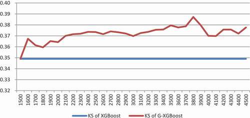
In addition, we test to amplify only the bad samples. Figure 9 shows, the curve of the average of KS value of the amplified sample set by adding only bad samples. It can be seen that the KS value increases sharply at beginning, then tends to grow slowly and remains in a stable state with minor fluctuations. Comparing with Figure 5, it can be found that the experimental results of the two amplification methods are similar. The KS values corresponding to the method in Figure 5 is more stable, and the KS values of the amplification method in Figure 9 is promoted faster at the initial stage of KS.

Figure 9. KS under only using bad samples to amplify the sample set.

In practice, loan institutions will formulate rules and strategies based on the distribution of SMEs with different risk prediction probabilities and the proportion of good and bad enterprises ratio. For enterprises with very bad prediction probabilities, direct rejection can be considered. At the same time, high-quality enterprises of low risk, can be graded based on the predicted results. Different SMEs can have different values, which can improve the overall pass rate and reduce the risk.

Conclusion

In this work, the GAN is applied to the model of SMEs credit risk to solve the problems such as small sample size, unbalanced sample distribution and difficult data acquisition in the currently available credit risk models. Through a range of experiments, it is found that the amplified sample set made by GAN generated samples can improve the performance of XGBoost model. The G-XGBoost model has significantly higher KS values than the XGBoost model, is better at differentiating credit risks, and has slightly better predictive accuracy than the XGBoost model. Meanwhile, it is found that, by adding bad samples alone, it is possible to use less samples to solve the problem of unbalanced samples and improve the model effect. In reality, there is no perfect optimal proportion to increase the sample size. We can increase the sample size of different categories in the same proportion, or appropriately increase the sample data with a relatively small proportion to expand the sample size according to the specific needs.

The amplified sample set based on GAN model might be applied not only to the XGBoost model, but the method can also be considered in constructing the credit risk model by combining score card, neural network and other models. This remains as the future works.

Disclosure Statement

No potential conflict of interest was reported by the author(s).

References

- Andrade, F. W. M., and A. L. Sicsú. 2008. A credit risk model for consumer loan portfolios. Latin American Business Review 8 (3):75–91. doi:https://doi.org/10.1080/10978520802035430.
- Antoniou, A., A. Storkey, and H. Edwards. 2018. Data augmentation generative adversarial networks, 1-14. [online] Available: https://arxiv.org/abs/1711.04340.
- Boz, Z., D. Gunnec, S. I. Birbil, and M. K. Öztürk. 2018. Reassessment and monitoring of loan applications with machine learning. Applied Artificial Intelligence 32 (9–10):939–55. doi:https://doi.org/10.1080/08839514.2018.1525517.
- Chen, T. Q., and C. Guestrin. 2016. Xgboost: A scalable tree boosting system. Proceedings of the 22nd ACM SIGKDD International Conference on Knowledge Discovery and Data Mining, San Francisco, USA, 785–94. [online] Available: https://arxiv.org/abs/1603.02754.
- Chen, Y. Z., Y. S. Wang, D. Kirschen, and B. Zhang. 2018. Model-free renewable scenario generation using generative adversarial networks. IEEE Transactions on Power Systems 33 (3):3265–75. doi:https://doi.org/10.1109/TPWRS.2018.2794541.
- Cheng, Z. 2014. The key to the healthy development of internet finance lies in risk management. Enterprise Reform and Management 9:144.
- Chi, G. T., M. D. Pan, and F. Qi. 2014. A credit rating model for analyzing bank customers based on small sample. The Journal of Quantitative & Technical Economics 6:102–16.
- Feng, G. Q., D. L. Cui, K. Q. Zhu, and Q. Zhang. 2019. Research of modeling with small sample for complex problem. Control Engineering of China 26 (11):2013–18.
- Frid-Adar, M., E. Klang, M. Amitai, J. Goldberger, and H. Greenspan. 2018. Synthetic data augmentation using GAN for improved liver lesion classification. 2018 IEEE 15th International Symposium on Biomedical Imaging (ISBI 2018), Washington, DC, USA, 289–93. doi: https://doi.org/10.1109/ISBI.2018.8363576.
- Friedman, J. H. 2001. Greedy function approximation: A gradient boosting machine. Annals of Statistics 29 (5):1189–232. doi:https://doi.org/10.1214/aos/1013203451.
- Gao, Q., and Z. H. Jiang. 2019. Amplification of small sample library based on GAN equivalent model. Electrical Measurement & Instrumentation 56 (6):76-81.
- Goodfellow, I. J., J. Pouget-Abadie, M. Mirza, B. Xu, D. Warde-Farley, S. Ozair, A. Courville, and Y. Bengio. 2014. Generative Adversarial Networks, Advances in Neural Information Processing Systems, 3:2672–80. [online] Available: https://arxiv.org/abs/1406.2661.
- Gupta, A., J. Johnson, F. F. Li, S. Savarese, and A. Alahi. 2018. Social GAN: Socially acceptable trajectories With Generative Adversarial Networks. 2018 IEEE/CVF Conference on Computer Vision and Pattern Recognition, 2255–64. Salt Lake City, UT. doi: https://doi.org/10.1109/CVPR.2018.00240.
- Hindistan, Y. S., B. A. Aiyakogu, A. M. Rezaeinazhad, H. E. Korkmaz, and H. Dag. 2019. Alternative credit scoring and classification employing machine learning techniques on a big data platform. 2019 4th International Conference on Computer Science and Engineering (UBMK), Samsun, Turkey, 1–4. doi: https://doi.org/10.1109/UBMK.2019.8907113.
- Jin, P. H. 2003. Medical statistical method, vol. 46. Shanghai: Fudan University Press.
- Kruppa, J., A. Schwarz, G. Arminger, and A. Ziegler. 2013. Consumer credit risk: Individual probability estimates using machine learning. Expert Systems with Applications 40 (13):5125–31. doi:https://doi.org/10.1016/j.eswa.2013.03.019.
- Lee, Y. H., and S. Z. Cho. 2020. Design of semantic-based colorization of graphical user interface through conditional generative adversarial nets. International Journal of Human–Computer Interaction 36 (8):699–708. doi:https://doi.org/10.1080/10447318.2019.1680921.
- Li, C. Y. 2019a. The influence of sample size change on the prediction accuracy of shanghai stock index. Henan Science and Technology 28:8–10.
- Li, Y. 2019b. Credit risk prediction based on machine learning methods. 2019 14th International Conference on Computer Science & Education (ICCSE), Toronto, Canada, 1011–13.
- Li, Z. J., F. Ju, C. B. Xiu, and G. H. Qiao. 2016. The construction of bank credit risk small sample rating model. Statistics and Decision 453 (9):41–45.
- Liu, Z. H., Z. G. Huang, and H. L. Xie. 2019. Is risk management with big data effective? —Comparison and analysis based on statistics score card and machine learning model. Statistics & Information Forum 34 (9): 18-26.
- Luo, C., D. Wu, and D. Wu. 2016. A deep learning approach for credit scoring using credit default swaps. Engineering Applications of Artificial Intelligence 65 (32). doi: https://doi.org/10.1016/j.engappai.2016.12.002.
- Ma, L. 2019. Research on innovation of financing model and risk management of small and micro enterprises under the background of internet finance. Institute of Management Science and Industrial Engineering (ISMEEM), Hanoi, Vietnam, 125–29.
- Mamdouh, R. 2011. Credit risk scorecards: Development and implementation using SAS, USA: Lulu.com.
- Mehta, K., Z. Kobti, K. A. Pfaff, and S. Fox. 2019. Data augmentation using CA evolved GANs. 2019 IEEE Symposium on Computers and Communications (ISCC), Barcelona, Spain, 1087–92. doi: https://doi.org/10.1109/ISCC47284.2019.8969638.
- Mirza, M., and S. Osindero. 2014. Conditional Generative Adversarial Nets. [online] Available: https://arxiv.org/abs/1411.1784.
- Nedellec, C., J. Correia, J. Ferreira, and E. Costa. 1994. Machine learning goes to the bank. Applied Artificial Intelligence 8 (4):593–615. doi:https://doi.org/10.1080/08839519408945461.
- Qiu, W. Y. 2019. Credit risk prediction in an imbalanced social lending environment based on XGBoost. 2019 5th International Conference on Big Data and Information Analytics (BigDIA), 150–56. Kunming, China. doi: https://doi.org/10.1109/BigDIA.2019.8802747.
- Radford, A., L. Metz, and S. Chintala. 2016. Unsupervised representation learning with deep convolutional generative adversarial networks. Computer Science, Proc. Int. Conf. Learn. Represent., San Juan, Puerto Rico [online] Available: https://arxiv.org/abs/1511.06434.
- Rahbar, M., M. Mahdavinejad, M. Bemanian, A. H. Davaie Markazi, and L. Hovestadt. 2019. Generating synthetic space allocation probability layouts based on trained conditional-GANs. Applied Artificial Intelligence 33 (8):689–705. doi:https://doi.org/10.1080/08839514.2019.1592919.
- Ratliff, L. J., S. A. Burden, and S. S. Sastry. 2016. On the characterization of local nash equilibria in continuous games. IEEE Transactions on Automatic Control 61 (8):2301–07. doi:https://doi.org/10.1109/TAC.2016.2583518.
- Shukla, U. P., and S. J. Nanda. 2019. Designing of a risk assessment model for issuing credit card using parallel social spider algorithm. Applied Artificial Intelligence 33 (3):191–207. doi:https://doi.org/10.1080/08839514.2018.1537229.
- Tran, K., T. Duong, and Q. Ho. 2016. A combination of genetic programming and deep learning. Future Technologies Conference (FTC), San Francisco, CA, USA, 145–49. doi: https://doi.org/10.1109/FTC.2016.7821603.
- Wang, B., Y. Kong, T. T. Zhang, D. P. Liu, and L. J. Ning. 2019a. Integration of unsupervised and supervised machine learning algorithms for credit risk assessment. Expert Systems with Applications 128:301–15. doi:https://doi.org/10.1016/j.eswa.2019.02.033.
- Wang, C. Y., C. Xu, X. Yao, and D. C. Tao. 2019b. Evolutionary generative adversarial networks. IEEE Transactions on Evolutionary Computation. [online] Available: https://arxiv.org/abs/1803.00657
- Wang, G. X., W. X. Kang, Q. X. Wu, Z. Y. Wang, and J. B. Gao. 2018. Generative adversarial network (GAN) based data augmentation for palmprint recognition. 2018 Digital Image Computing: Techniques and Applications (DICTA), 1–7. Canberra, Australia. doi: https://doi.org/10.1109/DICTA.2018.8615782.
- Wang, H. X., J. D. Zhong, D. F. Zhang, and X. Y. Zou. 2017. A new classification algorithm for the bank customer credit rating. 2017 Ninth International Conference on Advanced Computational Intelligence (ICACI) IEEE, Doha, Qatar, 143–48. doi: https://doi.org/10.1109/ICACI.2017.7974499.
- Wiese, M., R. Knobloch, R. Korn, and P. Kretschmer. 2020. Quant GANs: Deep generation of financial time series. Quantitative Finance 1–22. doi:https://doi.org/10.1080/14697688.2020.1730426.
- Wiginton, J. 1980. A note on the comparison of logit and discriminant models of consumer credit behavior. The Journal of Financial and Quantitative Analysis 15 (3):757–70. doi:https://doi.org/10.2307/2330408.
- Zhang, D., H. Huang, Q. Chen, and Y. Jiang. 2007. A comparison study of credit scoring models. Third International Conference of Natural Computation, Haikou, China.
- Zheng, L. C. 2014. Internet finance in China: Models, impact, nature and the risks. International Economic Review 5:103–18.