Artificial Intelligence Methods: Toward a New Decision Making Tool

ABSTRACT

This work is based on a mixe between the dynamics of investor decision making and the effectiveness of the forecasting models used to model market movements. Thus, it appears that the determination of adequate models can help to explain the behavior of agents and result to easier decision making through the anticipation of future prices. For this reason, we will use artificial intelligence models, in particular Machine Learning and Deep Learning algorithms, in order to better understand the variation of asset prices and their future evolution. In order to do so, we will use Recurrent Neural Networks (RNN), which has proven to be very suitable in the case of the Moroccan banking sector.

The comparison between classical models and advanced artificial intelligence (AI) algorithms has demonstrated the inadequacy of classical statistical models. The latter are based on certain assumptions not verified in the framework of financial series, which reduces the capacity of classical models to correctly predict new data. The integration of AI has also made it possible to overcome the assumption of market efficiency by modeling the behavior of irrational agents, who trade on rumors and false news.

Introduction

For several decades, IT tools have undergone rapid and remarkable development, which has enabled companies to improve their competitiveness on the market and become increasingly innovative. The field of Artificial Intelligence (AI), aims to reproduce human intelligence and performs tasks requiring the use of computers, hence its name “artificial.” In this sense, Machine Learning is currently the dominant trend. Figure 1 Simply put, AI enables computers to make forecasts of customer demand and decision-making based on large amounts of data. Figure 2 As a result, the potential of AI gradually increases as machines learn and refine their intelligence and predictive capabilities.

Figure 1. Algorithms of the learning machine .²

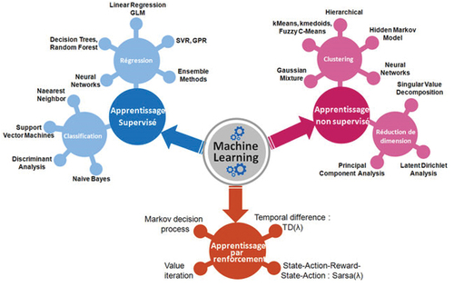
Figure 2. Data sets.

Figure 3. Example of a decision tree (AD).⁴

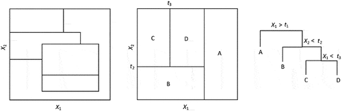
Figure 4. Structure of the neural network.

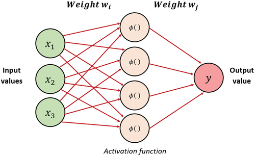
Figure 5. Support vector regression.

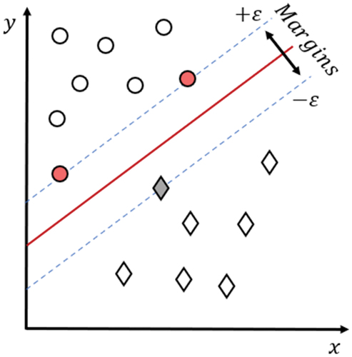
Figure 6. Forecast of the price index by the different models.

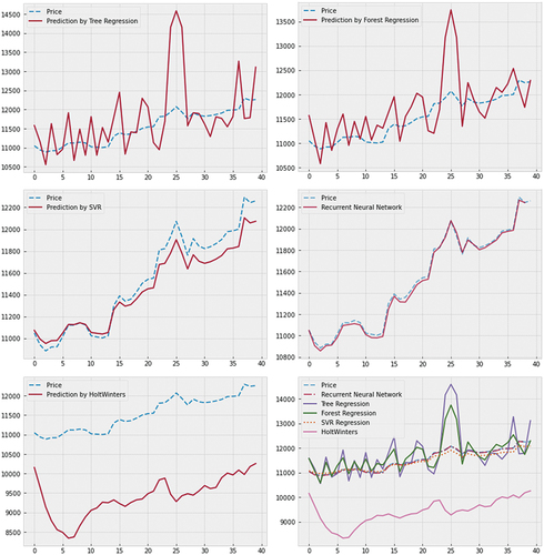
Table 1. Descriptive statistics of the price index

	Mean	Std	Median	Kurtosis	Skewness	Jarque-Bera
Price	11 828.94	1 474.18	11 445.22	−0.63	0.60	228.5

Table 2. Parameters of the selected models

Model	Parameter
Tree regression	$depth=36$	$leaves=2882$
Forest regression	$boostrap=True$	$n\mathrm{\_}estimators=100$
SVM	$kernel=poly$	$degree=3$
Neural network (LSTM)	$4layers$	$50neurons/layer$
	$epochs=100$	$optimizer=adam$
Holt-Winters	$method=heuristic$

Table 3. Quadratic error model average

Model	$MSE$
Tree Regression	$651641.78$
Forest Regression	$252295.83$
SVR	$13076.54$
RNN	$12\hspace{0.17em}054.14$
Holt-Winters	$4637230.18$

In finance, the applications of AI are multiple, namely: fraud detection, risk management, portfolio management, etc. Figure 3 Investment firms rely on algorithms based on complex probabilistic models (stochastic discrete-time or continuous processes) to determine future market trends. Figure 4 Machine Learning as a domain of AI guides decision making based on the predictive power of the model. As a result, machines are very powerful in this respect, as they can teach models to observe trends in past data and predict how these trends might repeat in the future.

If anomalies such as financial crises exist in past data, a machine can be taught to study the behavior of data changes in order to detect the triggers of these anomalies (pre-crisis recession) and predict them in its future forecasts. Moreover, depending on each individual’s risk aversion, Figure 5 AI can suggest specific weights, thus enabling the creation of a portfolio that meets investor demand.

The objective of this article is to understand the behavior of the financial series, as well as to manage to implement a model reflecting the future evolution of the prices of the Moroccan banking sector index, Figure 6 in order to help investors in their decision making.

The remainder of this work is organized as follows: Section 2 presents a brief overview of the literature and explains the interest in moving from classical models to intelligent models. Section 3 describes the models used in this study and the data and variables used in the experiment. Section 4 develops the results obtained. Section 5 closes the article with a conclusion and suggestions for future research.

Generalities and Concepts

The financial market is a place of competition between the supply and demand of financial assets, in which investors intervene through their portfolios. Access to this market forces them to bear the risk of over- or undervaluation of their assets. Table 1 According to a study by S&P Global, the most volatile market sectors during 2010 (period between 31 December 2009 and 31 December 2019) have suffered the most from the fast changes in oil prices. We list here, in descending order, the eight most important sectors with the largest standard deviations: Energy, Commodities, Financials, Technology, Consumer Discretionary, Communication Services, Health Care, Utilities.¹

Relevant Works

Several works have attempted to predict the daily variation in stock prices using the generalized linear model, autoregressive (AR), Table 2 Autoregressive Integrated Moving Average (ARIMA), or Bayesian regression.

Some authors such as (Velankar, Valecha, and Maji 2018) have used Bayesian regression and generalized linear regression to determine the daily trends of the bitcoin market. Table 3 The result achieved an accuracy of 51%.

Other authors have used time series models to predict future price changes. The work of (Ariyo et al., 2014) is based on Autoregressive Integrated Moving Average (ARIMA) models, especially its simplified form (ARMA), to provide investors with a short-term prediction that could facilitate the decision making process. However, the ARIMA model only allows for very short-term predictions and is sensitive to a sudden change in stock prices. Such a variation can be due to a financial crisis or new information on the financial market. Moreover, ARIMA is a linear statistical model that is based on fundamental assumptions (stationarity, normality, linearity, etc.). The same is true for the GARCH model, which only predicts risk according to a risk indicator such as the variance.

Recent work (Lamothe-Fernández et al. 2020; Luca and Honchar 2017; McNally, Roche, and Caton 2018; Milosevic 2016; Pudaruth 2014) has attempted to overcome the limitations of classical statistical models. They used artificial intelligence techniques, specifically machine learning and deep learning, in predicting future prices.

The work of (McNally, Roche, and Caton 2018) had as its objective, the comparison between a simple recurrent neural network (RNN), a long-term memory network (LSTM), and the Autoregressive method (ARIMA). The results show a clear improvement of the LSTM model over a simple recurrent network (RNN) and an inferiority of the ARIMA model over the LSTM and RNN. As a result, deep learning methods, which do not require assumptions about the distribution of the data, have outperformed classical ARIMA prediction.

Finally, other works, such as those of (Lamothe-Fernández et al. 2020), have used other techniques of artificial intelligence based on the combination of several learning methods to predict the price of bitcoin. We talk about hybrid models such as the Deep Recurrent Convolutional Neural Network (DRCNN) model that combines two algorithms: the convolutional neural network and the recurrent neural network.

Toward Intelligent Modeling

The modeling of risk (of volatility) has evolved a lot over time, going from the models of the economists of uncertainty, such as the CAPM, to the models proposed by econometricians and statisticians such as the GARCH models. This evolution and plurality of models is due to the understanding of new facts relating to the behavior of volatility on the financial markets and the evolution of research in financial econometric modeling. However, modeling using these models assumes that the market is efficient and that the agent is rational, yet market efficiency remains a simplifying assumption that does not allow the real behavior of agents to be taken into account. The use of more sophisticated AI models seems to be of crucial importance in order to model the behavior of irrational agents who trade on rumors and false news.

As mentioned above, the financial market is influenced by the behavior of agents, which is reflected in high asset volatility. Thus, one is often faced with many parameters to correctly write the volatility process of an asset return (Tadjeddine 2013).

Generally, GARCH (Generalized Autoregressive Conditional Heteroskedasticity) models are used to model asset volatility as well as the asymmetry of the distribution (leptokurtic and platikurtic) of returns. It is with this objective in mind that studies of different assets work with returns and not with prices, for two essential points:

• Any modeling of the price history with the aim of projecting itself into the future will be incorrect, and this is because certain properties of price processes do not remain constant over time. Reference is made to non-stationarity, and thus one prefers to use yield processes that have stationarity as a characteristic.

• The notion of correlation stipulates the existence of a temporal dependence between an observation at the present moment and its past history.

Investors often rely on econometric models that are based on a specific model and data set. Indeed, the parameters of a regression are calculated using an algebraic formula and the best linear unbiased estimator (BLUE) of the coefficients is generally given by the ordinary least squares (OLS) estimator or the maximum likelihood (ML) if certain assumptions are met. However, the latter are often rejected in finance, so that traditional statistical methods based on these assumptions cannot always be applied to market finance.

It is then extremely difficult to predict future volatility, and even more so future price volatility, without the use of advanced quantitative techniques. Hence the need to have a dynamic, evolving system that is capable of learning continuously, as new data is incorporated, and to optimize the investment strategy accordingly. It is in this perspective that the introduction of artificial intelligence (AI) has made it possible to overcome the classical assumptions of linear models (stationarity, normality, etc.). These include Machine Learning and Deep Learning models, which have the ability to adapt to changes in the properties of financial time series.

Machine Learning (ML) is a branch of artificial intelligence that consists of programming algorithms to learn automatically from data and past experiences or through interaction with the environment. What makes machine learning really useful is the fact that the algorithm can “learn” and adapt its results to new data without any prior programming.

Most of the techniques used in Machine Learning (a field of AI), are based on mathematical and statistical theories (advanced statistics, decision trees, Bayesian networks, neural networks, …) which have been known for about fifty years or more. AI considerably improves the understanding of human language and emotions, taking modeling to a whole new level. Thanks to artificial intelligence, we can also create models that study the behavior of investors and guide their decision making. There are several ways to learn automatically from the available data. The figure below gives a summary of the most common types of machine learning:

• Supervised learning: allows the machine to learn how to perform tasks from a set of data (examples that the machine must study). It is the most popular algorithm in Machine Learning and Deep Learning. In this learning mode, the main objective is to extract the links between one or more vectors (explanatory variables) and one or more output values also known as predictive variables (Mifdal 2019).

• Unsupervised learning: unlike supervised learning, this type of learning does not require a variable to be explained. It is completely autonomous and is generally used for classification and clustering. The algorithm looks for similar characteristics and properties in the database, as well as differences within them. It thus groups them into different homogeneous categories.

• Reinforcement learning: allows an agent to learn how to behave in an environment full of errors. In other words, the algorithm observes the results of actions and learns from these errors when a bad result occurs. This is known as the reward principle, which looks for the optimal behavior adopted in order to maximize the reward. This is a totally different way of learning than classification or planning (we don’t know the environment yet and it can change) and it is done without supervision (Mifdal 2019). We invite the reader to read about Markovian decision processes and Bellman’s equations for more details (Afia, Abdellatif, and Garcia 2019; Aoun and El Afia 2014).

Methodology

Data

A large amount of data is required to report on investors’ decisions in terms of value creation. We used data collected from the Casablanca Stock Exchange database. We also carried out what is called “Data pre-processing” which is a data mining technique that consists of pre-processing data to ensure that there are no missing data or outliers. The data available is of course current prices or historical prices, but remember that the outcome of investment decisions made today depends on future price levels.

The empirical study presented in this paper inspects the predictive power of the different models of the Learning Machine applied to the Moroccan banking sector index. The data collected cover the period from January 2, 2009 to December 15, 2020 with a daily frequency, i.e. a total of 2974 observations after processing of non-listing days.³

In the following table we report descriptive statistics for the different series. These statistics highlight the non-normality of the data, especially from the values of the skewness and kurtosis coefficients. Moreover, the Jarque-Bera test confirms this idea and firmly rejects normality for the price index of the Moroccan banking sector. Moreover, we draw attention to the high variability of prices especially in periods of crisis and the non-stationarity of the series.

We now proceed to a selection of sets (creation of samples) from the price index in order to take into account the time dependence of prices in our series (Mifdal 2019). We therefore retain the following three sets:

• Learning: set which allows the algorithm to perform the task it is asked to do (prediction, classification, …) by learning and improving from a training set. This set represents the first 80% of observations;

• Validation: set which allows the model parameters to be optimized. It represents the next 18% of the data;

• Evaluation: set which is mainly used to evaluate the predictive performance of the models. It is made up of the remaining 2% of the observations.

With: (1) Training, (2) Validation and (3) Evaluation

There are many different algorithms. we need to choose a particular type of algorithm depending on the nature of the study, the task we wish to accomplish and the data available. We have trained, optimized and tested five algorithms which will be presented below.

Modeling

Decision Tree Regression

In machine learning, it is very common to model different scenarios according to the information available. In this sense, the decision tree is a relatively simple classification and prediction tool.

This approach reached its apogee with the CART (Classification and Regression Tree) method of Breiman and Ihaka (1984), it consists in the construction of a tree (decision sequences) where each branch represents a test result, and each leaf contains the value of the target variable (Ezzikouri and Mohamed, n.d.).

In practice, decision trees are constructed by choosing at each step an input variable that best shares all the information. Subsequently, it will be necessary to choose the separation variable on a node by testing the different possible input variables and selecting the one that maximizes a given criterion (Gini diversity index in the case of a classification or the Chi-2 test in the case of a regression). The process stops when the elements of a node have the same value for the target variable (DataScienceToday - ML Supervised, n.d.).

Neural Network

Artificial neural networks are more complex mathematical models than all other Machine Learning models based on the functioning of our own neurons (simulation of the behavior of biological neurons). They are used in different fields such as: prediction, classification, pattern recognition, feeling analysis and simulation of human behavior.

Generally, a neuron (or a node) is a process that may have one or more input signals with a weight that represents the strength of the connection to that node. The latter represents activation functions that will allow the neuron to pass information when it is activated. Finally, this neuron gives rise to one or more outputs which will be transmitted to the second layer of the neural network.

For a basic neural network, the Logistics function is used as an activation function. However, the use of other activation functions than the logistic (sigmoid) function such as the hyperbolic tangent function or the $Relu()$ function may be preferred to simplify the calculation and obtain a faster learning.

If our network has several layers called hidden layers, we link all the outputs of the neurons with all the inputs of all the neurons of the next layer. Thus, the more hidden layers the network has, the deeper the network is and the more robust the model is. It is this notion that leads us back to Deep Learning (Mostafa 2013).

The calculation performed by a neuron is performed in two steps:

• Calculation of the sum of inputs weighted by $\mathrm{\Sigma }{w}_i{x}_i$

• Pass this number to the neuron activation function

In order to obtain the desired behavior of the neural network, learning is carried out which allows the connection strength of each neuron to be modified. This leads to a modification of the behavior of the network. The objective is to determine a set of “$W$“ weights which minimize the total sum of errors ($min\mathrm{\Sigma }{e}_i$). However, developing such a complex function will create additional constraints at the study level in the sense that it will often require a large database, a longer model learning time and high computing power.

When temporal sequences are present, modeling with a simple artificial neural network loses its efficiency because it does not take into account the temporal dependence. The introduction of a recurrent neural network (RNN) overcomes this problem by introducing the notion of the internal memory of a network.

Financial series are temporal sequences where each observation depends on past realizations. We speak of the phenomenon of temporal autocorrelation. It is in this sense that the family of recurrent neural networks seems the most appropriate for the estimation and forecasting of this kind of sequences. This advantage is mainly based on the fact that the cells of the recurrent neural networks (RNN) take as input the data at time t and also the outputs of the data at time $t-1$.

However, recurrent neural networks have some limitations which are mainly summarized in the vanishing gradient problem which leads to the generation of several near zero values (Hochreiter 1998). Moreover, the simple recurrent network (SRN) only takes into account the near past and the distant past will have little (or no) impact on the estimate at time “$t$“. This problem is aggravated when the sequences have a significant length.

The solution to these problems lies in the Long short-term memory model (LSTM). It is a model of the family of recurrent networks which is the most used in practice because it allows to control the internal state according to the past. In addition, LSTM cells have the ability to maintain essential information and forget non-important information (Luca and Honchar 2017).

Support Vector Machine

The Support Vector Machine (SVM) algorithm is a supervised learning technique. Unlike linear regression, which minimizes the sum of the errors squared, this algorithm allows us to define a tolerable level of error in our model noted “ε.” Their objective is to separate the data into classes using a boundary. However, the data are rarely separable by a linear boundary, which is why SVMs are based on the “kernel” principle, which allows a projection of the observations in a hyperplane. Thus, by maximizing the margins (the tolerable error), we obtain a better result in the face of the noise generated by the estimation.

This problem may be solved by optimization techniques, in particular that of Lagrange multipliers. Assume the model:

$y=ax+b$

It will therefore be necessary to minimize:

$Min\frac{1}{2}{\left|\left|a\right|\right|}^2$

Under duress:

$y_i-a{x}_i-b\le \epsilon$

$a{x}_i+b-y_i\le \epsilon$

Finally, the performance of SVMs is comparable to that of a neural network when the choice of the kernel is in line with the data of the study.

Holt-Winters

Exponential smoothing is more about predicting a time series than modeling it. It is one of the most widely used smoothing methods and has been practised for more than half a century. It has undergone significant theoretical development over the last twenty years or so and is based on a model associated with a space-state representation and on the innovation filter (noise). It is easy to use and requires little data.

Many recent exponential smoothing methods are available on the various software packages dedicated to statistical computation. These methods start from a series decomposition into trend, seasonality and error, and propose a mechanism for updating the trend and seasonality when a new observation is available.

The aim of the method is to predict future values of the series, giving greater weight to the most recent observations; otherwise, the older the observations, the less they affect the forecast. This importance decreases exponentially. Hence the name of the method.

${\hat{y}}_{t+1}={\theta }_0{y}_t+{\theta }_1{y}_{t-1}+{\theta }_2{y}_{t-2}+\dots$

With ${\theta }_i=\alpha {\left(1-\alpha \right)}^i$ and $\alpha$ the smoothing constant. Hence the prediction of par:

${\hat{y}}_{t+1}=\alpha y_t+\alpha \left(1-\alpha \right)y_{t-1}+\alpha {\left(1-\alpha \right)}^2{y}_{t-2}+\dots$

It can easily be demonstrated by recurrence that:

${\hat{y}}_{t+1}=\alpha y_t+\left(1-\alpha \right){\hat{y}}_t$

This equation allows us to update the prediction when a new observation is available.

Holt-Winters’ method is a generalization of the exponential smoothing method in that it allows us to model the season in addition to the trend.

The three recurrent formulas known as update formulas:

$\left\{\begin{array}{c}{\hat{y}}_{t+1}=\alpha y_t-{\hat{S}}_{t-k}+\left(1-\alpha \right)\left({\hat{y}}_t+b_{t-1}\right)\\ \\ b_t=\beta \left({\hat{y}}_{t+1}-{\hat{y}}_t\right)+\left(1-\beta \right)b_{t-1}\\ \\ {\hat{S}}_t=\gamma \left(y_t-{\hat{y}}_{t+1}\right)+\left(1-\gamma \right){\hat{S}}_{t-k}\end{array}\right.$

Where ${\hat{S}}_t$ is the estimate of $S_t$ the seasonal of period $k$.

Results and Discussion

The estimation of our models necessarily involves identifying the parameters and attributes that will provide the best result from each model. In this way, we can make a comparison of the latter on data not provided by the learning data. It is new data (in particular the validation set) which will be able to highlight the real performance of the different algorithms (Kendi et al., 2012) .

Based on this observation, the parameters presented in the table below have enabled us to refine the hyperparameters of the model, in order to optimize the performance provided by the model for our series of studies (Moroccan banking sector index):

At the end we perform an estimate from the valuation set (data not known by our models) to see how prices change after changes in the data. Subsequently, the model-based forecast is obtained:

• We can see that the prediction by the Tree Regression algorithm (Figure 6.1) has a high variance of observations and subsequently a high volatility of predictions compared to other models. We can therefore reject this model as it varies more as the data changes, meaning that the model is not very robust to unusual change and suffers from underlearning.

• We draw the same conclusion for the Forest Regression algorithm (Figure 6.2). This conclusion is not surprising since the algorithm is an extension of the Tree Regression, which is why we obtain an even better result with respect to the variability of future observations but still insufficient.

• We obtain an interesting result with SVR algorithms and neural networks (LSTM) which present a robust prediction for data still unknown by the algorithm (figures 6.3 and 7.4). This result is simultaneously related to what we presented in the modeling section. However, there is an advantage of Recurrent Neural Networks over Support Vector Machine (SVM), in the sense that the prediction of RNNs fits perfectly with the real evolution of the price index. The analysis of the quadratic error confirms this result by demonstrating that the neural network model has a minimal quadratic error:

• Given the results obtained, we can conclude that the majority of our models, with the exception of the neural networks and partially the Vector Machine Support, suffer an underlearning and do not allow us to have a robust and reliable prediction. We therefore retain recurrent neural networks as a powerful forecasting model in the case of the Moroccan banking sector.

Conclusion

Based on the empirical results, we concluded that neural networks and Support Vector Regression (SVR) can reduce the mean square error (MSE) in financial series. Thus, we can refer to predict the future price of financial indices. This result is due to the fact that neural networks represent a deep learning method characterized by a strong theoretical background that has allowed them a great capacity of adaptation to market variations, which places them at the forefront of analysis tools in artificial intelligence.

On this basis, we have retained from this study that the integration of artificial intelligence models allows to overcome the obstacles and assumptions of classical models such as normality, information symmetry, stationarity, or market efficiency. These obstacles reduce the ability of classical models to correctly predict new data.

To test the effectiveness of this approach, six models have been designed, trained and evaluated on the basis of the mean square error (MSE) with daily data representing the price index of the Moroccan banking sector. We tested all six models and came to the conclusion that neural networks have better predictive power, which means that they can learn and adapt to market movements. These overall results demonstrate that the neural network approach, especially recurrent networks, can be an effective method for forecasting the stock market. Therefore, they can be used as a means of detecting future crises through the trend behavior of the market.

The investor will be able to predict the evolution of prices, which will guide his investment decision in order to achieve two objectives:

• Limit the risks incurred

• Maximizing the benefits of the investment

However, the complexity of neural networks means that training the model can take a significant amount of time (hours or even days) and requires very powerful machines. Also, the choice of the architecture of the artificial neural networks (number of hidden layers, number of neurons per hidden layer and their interconnection) presents a major difficulty and can impact the predictive power of the model. Moreover, we must be wary of the phenomenon of model overfitting, one of the causes for which the model can lose predictive performance. The model then generates predictions from past observations without any adaptation to new information.

As an extension to this work, we first consider optimizing the parameters and architecture of the neural network in order to determine the best applicable model on our data. Also, we can use optimization methods to find the ideal architecture. Second, we will consider applying our approach on other data from various stock markets, as we have focused on the Moroccan market, to make more comparisons.

Disclosure statement

No potential conflict of interest was reported by the author(s).

Notes

1. https://cutt.ly/fhCFTzb

2. https://www.groupe-hli.com/machine-learning-dans-industrie/

3. https://cutt.ly/vhCDMf2

4. http://cedric.cnam.fr/vertigo/cours/ml2/coursArbresDecision.html

References

- Afia, E., O. A. Abdellatif, and S. Garcia. 2019. Adaptive cooperation of multi-swarm particle swarm optimizer-based hidden Markov model. Progress in Artificial Intelligence 8 (4):101–116. doi:10.1007/s13748-019-00183-1.
- Aoun, O., and A. El Afia. 2014. ‘A Robust crew pairing based on multi-agent Markov decision processes’. In 2014 Second World Conference on Complex Systems (WCCS), 762–68, Agadir, Morocco. https://doi.org/10.1109/ICoCS.2014.7060940.
- Ariyo, A. A., A. Adewumi O., and E. C. K. Ayo. 2014. Stock price prediction using the ARIMA model . In 2014 UKSim-AMSS 16th International Conference on Computer Modelling and Simulation, 106–12. IEEE, Cambridge, UK.
- Breiman, L., and R. Ihaka. 1984. Nonlinear discriminant analysis via scaling and ACE. Department of Statistics, University of California.
- ‘DataScienceToday - ML Supervised’. n.d. Accessed 20 December 2020. https://datasciencetoday.net/index.php/fr/machine-learning/109-ml-sup
- Ezzikouri, H., and F. Mohamed. n.d. ‘Algorithmes de classification : ID3 & C4.5ʹ, 36.
- Hochreiter, S. 1998. The vanishing gradient problem during learning recurrent neural nets and problem solutions. International Journal of Uncertainty, Fuzziness and Knowledge-Based Systems 6(2): 107–116.
- Kendi, S., F. Laib, and M. S. Radjef. 2012. ‘Application des Réseaux de Neurones Récurrents à la Formation de Prix à Terme dans le cas de Deux Traders: Producteur-Consommateur’, 9.
- Lamothe-Fernández, P., D. Alaminos, P. Lamothe-López, and E. M. A. Fernández-Gámez. 2020. Deep learning methods for modeling bitcoin price. Mathematics 8 (8):1245. doi:10.3390/math8081245.
- Luca, D. P., and E. O. Honchar. 2017. Recurrent neural networks approach to the financial forecast of Google assets . International Journal of Mathematics and Computers in Simulation 11:7–13.
- McNally, S., J. Roche, and E. S. Caton. 2018. Predicting the price of bitcoin using machine learning . In 2018 26th euromicro international conference on parallel, distributed and network-based processing (PDP), 339–43. IEEE, Cambridge, UK.
- Mifdal, R. 2019. ‘Application des techniques d’apprentissage automatique pour la prédiction de la tendance des titres financiers’, 196.
- Milosevic, N. 2016. Equity forecast: Predicting long term stock price movement using machine learning . arXiv. preprint arXiv:1603.00751.
- Mostafa, E. L. H. A. C. H. L. O. U. F. I. 2013. ‘Les Apports de l’Intelligence Artificielle Aux Approches Probabilistes Pour l’Optimisation de Portefeuille d’Actifs Financiers’.
- Pudaruth, S. 2014. Predicting the price of used cars using machine learning techniques . Int. J. Inf. Comput. Technol 4 (7):753–64.
- Tadjeddine, Y. 2013. La finance comportementale. Idees Economiques Et Sociales N° 174 (4):16–25.
- Velankar, S., S. Valecha, and E. S. Maji. 2018. Bitcoin price prediction using machine learning . In 2018 20th International Conference on Advanced Communication Technology (ICACT), 144–47. IEEE, Abuja, Nigeria.