Energy Efficient Cluster Head Selection in Internet of Things Using Minimum Spanning Tree (EEMST)

ABSTRACT

Internet of things network lifetime and energy issues are some of the most important challenges in today’s smart world. Clustering would be an effective solution to this, as all nodes would be arranged into virtual clusters, while one node will serve as the cluster head. The right selection of the cluster head will reduce energy consumption dramatically. This concept is more crucial for the internet of things, which is being widely distributed in environments such as forests or the smart agriculture sector. In this paper, an Energy Efficient Minimum Spanning Tree algorithm (EEMST) is presented to select the optimal cluster head and data routing based on graph theory for a multihop Internet of Things. This algorithm calculates the Euclidean distance-based minimum spanning tree based on a weighted graph. As a result, we use a weighted minimum spanning tree to choose the optimal cluster head and accordingly determine the shortest path for data transmission between member nodes and the cluster head. The proposed EEMST algorithm provides the possibility of intracluster multihop routing and also the possibility of intercluster single-hop routing. The simulated experimental results approve a significant improvement of the proposed algorithm in the IoT systems’ lifetime compared to the baselines.

Introduction

Internet of Things (IoT) refers to a distributed system of interconnected instruments, wireless devices, people, agents and animals (Azad, Navimipour, and Rahmani 2020; Pourghebleh and Hayyolalam 2020; Elias et al. 2016; Peyravi and Keshavarzi 2009). Each element in the network has a unique identifier. A user-to-user and/or user-to-device communication quality and channels are one of the major issues to be assured in the IoT area (Keshavarzi, Haghighat, and Bohlouli 2017). Hence, people can closely interact with physical world according to real-time activity of sensor nodes. These nodes are low-power and multifunctional devices that could monitor various environmental factors such as ocean environment (Vo et al. 2021) and physical conditions such as pressure, temperature, sound and pollution.

Wireless Sensor Networks (WSNs) are crucial and fundamental requirements for implementing the vision of the IoT. It enables the information exchange between different parts of an IoT system. Limitations of battery power, storage capacity, bandwidth and processing separate this kind of network from other types. In terms of battery consumption, redundant data transferring tasks cause higher energy loose in the network. Therefore, it is vital to minimize redundant data transfer in order to decrease energy consumption and accordingly increase the network lifetime. WSNs have numerous applications, especially in cases where the use of traditional networks is not possible (Afshoon et al. 2020).

However, we use the term sensoric IoT for the network of IoT devices that consist of lightweight sensors, which have a short lifetime and are being used for monitoring the difficulty in reaching regions such as forests and/or smart farming areas (Behera et al. 2019; T. Han et al. 2019). It should be mentioned that the sensoric IoT consists of numerous sensor nodes that each node typically has been provided with a power source, usually a battery, a radio transmitter and a microprocessor. In general, the batteries in light weight sensors are nonrechargeable, so the energy efficiency is a major challenge in such networks (Nguyen et al. 2021). Consequently, new approaches play a key role in providing energy efficiency and increased lifetime of sensoric IoT devices (Hu et al. 2019; Praveen Kumar and Rajasekhara Babu 2019, 2019a). In this regard, various techniques, such as topology control (Li, Zhenjiang, and Vasilakos 2013; Zeng et al. 2013; X. M. Zhang et al. 2015), routing (Busch, Kannan, and Vasilakos 2012; Du et al. 2007; Meng et al. 2016) and security (Jing et al. 2014; Ozdemir and Xiao 2009), have been undertaken by researchers. One of the approaches that largely has been successful in the field of energy efficiency is the use of a hierarchical structure (T. Han et al. 2019; Hu et al. 2019; Cao et al. 2008; F. Chen et al. 2015; K. Han et al. 2013; Keshavarzi, Haghighat, and Bohlouli 2021).

Energy efficiency can be achieved in topology control by hierarchical arrangement of nodes that results in avoiding energy consumption because of direct long-distance communications (Keshavarzi, Haghighat, and Bohlouli 2020). In this regard, clustering of nodes is an important technique in relation to a hierarchical structure, which reduces bandwidth loss, congestion and IoT network error. This is because of less concurrent information transfer between the environment and the base station or sink for a reduced number of nodes (Lee and Cheng 2012). However, an efficient mathematical modeling of cluster head (CH) selection in IoT is not efficiently addressed in the state-of-the-art research.

Arranging regional nodes as a sort of a cluster results in efficient communication between nodes in the same cluster and its CH. Then, CHs collect information being sent by the nodes inside a corresponding cluster and often compress this information and then CHs send the collected information to the base station or sink. Therefore, selecting the proper CH can significantly reduce energy consumption and increase the lifetime of IoT (Liu et al. 2015; Xu et al. 2015; Behera et al. 2019; T. Han et al. 2019; Praveen Kumar and Rajasekhara Babu 2019a, 2019). Selecting the proper CH is as important and effective as the algorithm used for clustering because of the reduced connection traffic in the network and accordingly increased energy efficiency and network lifetime. The CH selection approaches can be grouped into two various types (Jafarizadeh, Keshavarzi, and Derikvand 2017):

The first method is introduced with clustering algorithms. The second group includes methods that propose algorithms on selecting the CH and are developed based on one of the first-order algorithms. They optimize the CH node selection process. It should be stated that output of these methods in practice is more efficient than the first method because most of the second-order algorithms are based on artificial intelligence techniques of solving optimization problems and methods that use analytics to realize an optimum solution (Jafarizadeh, Keshavarzi, and Derikvand 2017). In addition to clustering and CH selection techniques, energy efficiency routing techniques are required because of the limited computing, storage and battery power resources in IoT (Behera et al. 2019; Praveen Kumar and Rajasekhara Babu 2019a; Saravanan and Madheswaran 2014). Tree-based routing is used due to its energy efficiency in IoT (X. Wang and Qian 2012; J. Zhang et al. 2012; Zheng and Zhengbing 2010). In tree-based techniques, before the date is being transmitted, they select a root. In order to make a connection between modes, these techniques construct a hierarchical root between nodes. This tree-like IoT nodes’ path can be Minimum Spanning Tree (MST) (Behera et al. 2019; Saravanan and Madheswaran 2014).

Given a connected and undirected graph, a spanning tree of that graph is a subgraph that connects all the vertices together. A single graph can have many different spanning trees. An MST or minimum weight spanning tree for a weighted, connected, undirected graph is a spanning tree with a weight less than or equal to the weight of every other spanning tree. The weight of a spanning tree is the sum of weights given to each edge of the spanning tree. In general, the MST connects all sensor nodes in order to reduce energy consumption. This could happen by packet shortening the distance of packet transfers and/or reducing the number of packets to be transmitted (Saravanan and Madheswaran 2014). Although many works paid attention to CH selection, they usually considered very few parameters and neglected vital parameters such as total energy of all clusters’ nodes and total distance of a candidate node to all other alive nodes that exist in that cluster. Considering these parameters as criteria can decrease energy consumption and increase the lifetime of IoT systems. We propose a novel approach based on the graph theory to determine the CH node in IoT, which is approved through our experimental results to increase the IoT network lifetime expectancy in comparison with other methods. In particular, we notate an IoT in the form of a graph $G\left(V,E\right)$, where $V$ demonstrates a set of IoT nodes and $E$ ($E\subseteq V\times V$) corresponds to the links between IoT nodes (Zheng and Zhengbing 2010). It should be stated that the graphs are connected, simple, finite, nondirectional and do not consist of multiple edges or any loop,

$G\left(V,E\right)$ undirected if for all $v,w\in V$: $\left(v,w\right)\in E\iff \left(w,\hspace{0.17em}v\right)\in E$.

In the EEMST algorithm, at first, the MST based on the Euclidean distance is being built for the composed weighted graph of the multihop network and these spanning trees in addition to selecting the optimal CH are also employed for data routing from member nodes to the CH node.

The structure of this paper is organized as follows. In Section 2, some of the previous successful works, each with a different approach, have been introduced. In section 3, the description of the proposed algorithm, the creation of a weighted graph, the MST, and selection of the CH node are explained in detail. In section 4, updating the energy level of the nodes is explained. In the next section, we describe the simulation of the proposed algorithm and evaluate the output performance; the final part is related to the conclusion and future works.

Related Work

As stated earlier, in the first-order algorithms, the primary purpose was the clustering, but implicitly, a method was introduced for selecting the CH node. LEACH (Heinzelman, Chandrakasan, and Balakrishnan 2000) is one of the most common algorithms in this area. This algorithm consists of two steps: (1) the setup phase, in which each node is being selected as CH with a certain probability, and (2) the stable state phase, in which each existing node in the cluster transfers collected data to the corresponding CH. After collecting data, each CH transfers the data directly to the base station. The probability of each node to become CH independently depends on a possible value, low-battery nodes.

Moreover, the PEGASIS well-known protocol (Lindsey and Raghavendra 2002) is one of the LEACH developments that uses a chain of nodes to start data transmission from the most far node considering that each node would send its data to the most closed neighbor. This algorithm balances the energy consumption inside a chain, but results in an increased data transmission delays and is consequently not suitable for large-scale networks. HEED, a distributed clustering method, is proposed for long-lifetime ad hoc networks (Younis and Fahmy 2004). This protocol allows single-hop communication inside every cluster and multihop communication between CHs and the base station.

Selecting the CH depends on the cost of intracluster communications and the remaining energy, unlike LEACH, which selects clusters randomly, the remaining energy is used to select the primary set of CHs and the cost of intracluster communications is used in order to decide to join a cluster. This cost is based on the closeness of the node or node degree to the neighbor. In addition to the abovementioned algorithms, other methods for selecting the CH node have been introduced. Varghese (Varghese 2016) proposed an algorithm to select the CH using various parameters such as high energy, high throughput and minimum distance from the base station, besides considering the potential of each node.

In the second-order methods, some general approaches, such as evolutionary algorithms, machine learning, fuzzy systems, etc., are used. For example, in Pal et al. 2015, the genetic algorithm is used to select the CH and the fitness function is composed based on the parameters such as remaining energy, the number of CHs, the total intracluster communications distances and the total CH distances to the base station. Fuzzy logic is also another approach to select a CH and in Gajjar, Sarkar, and Dasgupta 2014 and Barolli et al. 2012, the fuzzy logic-based CH selection method has been proposed for WSNs. An ant colony optimization technique has also recently been used to solve many of the optimization problems of different areas of the WSN and has provided a good return. In Sharma et al. 2014, an algorithm based on an ant colony technique is introduced. The authors have used ACO in IoT routing and generate the optimal route using the probable approach and the amount of pheromone from the source node to the sink. In this algorithm, the CHs are randomly selected as the LEACH setup phase. A particle congestion optimization technique is another well-known optimization technique that is effective for selecting CH nodes. In Ni et al. 2015, a new method for selecting a CH is introduced, which uses the traditional PSO algorithm to select the CH and fuzzy clustering (Chiu 1994) for initial clustering of the nodes.

In Jafarizadeh, Keshavarzi, and Derikvand 2017, the authors use the Naïve Bayes function, as a data mining technique, to determine the CH node in a WSN. Parameters such as the remaining energy of the node and the total local distance of the member nodes to the CH node are used to select the appropriate CH. An intracluster spanning tree (Lachowski et al. 2015) can also optimize the energy efficiency. Furthermore, a clustering algorithm is provided in C. Li et al. 2011 by means of spanning trees. In this way, they claim that they have succeeded in increasing the scalability of their clustering algorithm and accordingly extending their network lifetime. The BASA-WMST method is proposed in Saravanan and Madheswaran 2014, which is a Bee Algorithm-Simulated Annealing Weighted Minimal Spanning Tree and is a hybrid evolutionary algorithm for data routing in IoT. In this method, there is random deployment of sensor nodes in the field. The nodes are divided into clusters and the best possible number of clusters is estimated along with the optimal data route. This algorithm calculates the MST from the weighted graph for a multihop network; the weighted MST is used to determine the shortest path between the member nodes of the cluster. The most important algorithms for solving shortest path problems are as follows (Chapuis et al. 2017):

• Breadth-first search and depth-first search refer to different search orders; for depth-first search, instances can be found where their naive implementation does not find an optimal solution or does not terminate.

• Dijkstra’s algorithm solves the Single-Source Shortest Path problem if all edge weights are greater than or equal to zero. Without worsening the runtime complexity, this algorithm can, in fact, compute the shortest paths from given start points to all other nodes.

• The Bellman-Ford algorithm also solves the Single-Source Shortest Path problem, but in contrast to Dijkstra’s algorithm, edge weights may be negative.

• The Floyd-Warshall algorithm solves the All Pairs Shortest Path problem.

• The A* algorithm solves the Single-Source Shortest Path problem for non-negative edge costs.

The weights of the edges of the network are not constant and change according to the energy levels of sensor nodes and the tree is optimized using the bee algorithm-simulated annealing algorithm. In Hussain and Islam 2007, an Energy Efficient Spanning Tree (EESR) algorithm was proposed, which supports multihop routing in homogeneous networks and increases the network lifetime. The EESR considers the location of the sensor nodes and base station and produces a series of routing paths consisting of the appropriate number of rounds. The results show that the EESR algorithm outperforms in relation to increasing the network lifetime. Another CH selection for sensoric IoT has been proposed in J. Chen and Shen 2008, which is entitled More Energy-efficient LEACH for Large-scale IoT (MELEACH-L) and is divided into 4 various steps. These steps are sequential and run each after another. The first step starts with the CH selection, followed by the backbone and spanning tree constructions. In the last step, the data are being collected. They used the Energy-aware Virtual Backbone Tree (EVBT) algorithm (Zhou, Marshall, and Th 2005) in the second and third steps for spanning tree construction.

Similarly, there is also a Base station Controlled Dynamic Clustering Protocol (BCDCP). In this method, CHs are being connected by means of the spanning tree and sink functions (Muruganathan et al. 2005). As an improved version of the BCDCP, Huang, Xiaowei, and Jing 2006 proposes the Dynamic Minimal Spanning Tree Routing Protocol (DMSTRP). This protocol is dedicated for large WSNs and uses MSTs. This protocol replaces clubs in the intra- and interclusters. Furthermore, data fusion is used in this protocol along with the tree-like path and reduced collision. In W. Wang et al. 2011, the CTPEDCA protocol is introduced the use of the full distribution in hierarchical IoT. CTPEDCA has combined the spanning tree strategy and clustering. The CHs are being selected using the same strategy as the LEACH protocol. In each round, once the CHs are selected, they construct a spanning tree. A CH with the highest energy consumption is being selected as a root of the spanning tree. The CHs deliver aggregated data along the tree and finally, the root node delivers data to the base station.

In Praveen Kumar and Rajasekhara Babu 2019a, the authors proposed a hybrid optimal CH selection approach for WSN–IoT that uses Moth Flame Optimization (MFO) and Ant Lion Optimization (ALO) algorithms. The main objective in this work is to select CH by retaining the energy of the node and making a balance in the temperature and workload of IoT devices. In this work, the CH selection models have been investigated by means of the distance and energy, latency, load and temperature constrained selection. In the distance constrained selection method, target nodes should be located in the specific distance to the CH. The same applies to the energy constrained selection in terms of energy discharging in IoT networks. It should be stated that the delay, temperature and loads should be minimized as well. To solve these issues, they proposed a hybrid approach. The performance of the aforementioned hybrid approach has enhanced the lifetime of the WSN–IoT network.

Another approach is given in Behera et al. 2019, which uses rotational adjustment of the CH position between various nodes through comparing the higher energy consumption. The parameters that are being considered in this method are initial and remained energy of the individual node as well as an optimal number of CHs. The remained energy of non-CH devices is being evaluated in the final round. Accordingly, the priority of selecting the CH in the next round is given to a node with higher energy consumption. This results in having a longer alive network and preventing it to die in terms of energy. Their results through the simulation show improvement in the network lifetime, remained energy, throughput and sent packets to the base station.

In Praveen Kumar and Rajasekhara Babu 2019, the self-adaptive whale optimization algorithm (SAWOA) has been proposed. This method considers CH selection with respect to the energy and uses clustering protocols in the WSN-IoT. Similarly, energy consumption, distance and latency of nodes as well as temperature and load of nodes in the IoT Network have been considered and key factors. The key consideration here is selection of a node as CH with the maximum energy and minimum distance and latency. In terms of IoT devices, load and temperature are also being considered. The main important achievement of this work is higher lifetime of the network using this selection method. In Table 1, a number of clustering and CH selection algorithms proposed in this section and the EEMST algorithm will be compared.

Table 1. Comparison of clustering algorithms and CH selection in IoT

Algorithm	Intra-/intercluster routing	CH selection parameters	Advantages	Disadvantages
LEACH (Heinzelman, Chandrakasan, and Balakrishnan 2000)	Single-hop/Single-hop	Selection of the CH is random regardless of the remaining energy of the nodes.	1. Distribution of energy loads on network sensors 2. Avoiding rapid discharge of the battery	1. Not considering the remained energy of nodes in the selection of the CH 2. Nodes with less energy also have the chance to be CH
PEGASIS(Lindsey and Raghavendra 2002)	Multihop/Single-hop		1. Reducing the overhead of clustering using a chain method 2. Reducing energy consumption 3. Reducing data transfer to BS	1. High latency in the final transfer of data to the base station 2. Not suitable for large-scale networks
HEED(Younis and Fahmy 2004)	Single-hop/multihop	1. Intracluster communication cost 2. Remaining energy	1. Cause the little overhead of messages 2. Ensure the connection between the clustered network and the effective increase in the lifetime of a network	1. If the CHs are too far away, energy consumption is significant. 2. It needs to be aware of the entire network in order to determine the cost of intracluster communications
Naïve Bayes (Jafarizadeh, Keshavarzi, and Derikvand 2017)	Single-hop/Single-hop	1. Remained energy of the node 2. Total local distance of a member node to the CH	1. Increasing network lifetime 2. Use of the Bays consistent loss function in data mining is very suitable for obtaining minimum and maximum values	1. Death of the first nodes in elementary rounds 2. Lack of consuming energy distribution on nodes 3. Discharging the battery of CH rapidly
Hybrid Algorithm(Praveen Kumar and Rajasekhara Babu 2019a)	Single-hop/Single-hop	1. Delay, distance and Energy in the WSN 2. The load of IoT devices as well as the Temperature	1. Prolonging network lifetime 2. Improved CH selection performance among IoT devices in the WSN–IoT network 3. Preserved energy of devices by minimized delay and distance 4. Balanced load and temperature of IoT devices	1. Using single-hop routing causes increasing energy consumption 2. Doesn’t consider number of alive devices in the cluster, total energy of clusters’ alive devices and total node distances to alive nodes in the CH selection
SAWOA algorithm(Praveen Kumar and Rajasekhara Babu 2019)	Single-hop/Single-hop	1. Energy, distance and delay of sensor nodes in WSN 2. Load and temperature of IoT devices	1. Enhancing lifetime of the network by balancing the number of alive nodes and normalized energy of the network	1. Using single-hop routing causes an increase in energy consumption 2. Does not consider the number of alive nodes in the cluster, total energy of clusters’ alive nodes and total node distances to alive nodes in the CH selection
R-LEACH(Behera et al. 2019)	Single-hop/Single-hop or Multihop	1. Initial energy 2. Remained energy of the individual node 3. Optimal number of CHs in the network	1. Extended network lifetime through controlling energy dissipation of the network 2. Enhancing the throughput, remained energy and sent packets to the base station	1. Does not consider the number of alive nodes in the cluster, total energy of clusters’ alive nodes and total node distances to alive nodes in the CH selection
EEMST Algorithm	Multihop/Single- hop	1. Remaining energy of the node 2. Total energy of clusters’ alive nodes 3.Total node distances to alive neighboring nodes in the MST 4. Total node distances to alive nodes in cluster 5. Node distance to the base station 6. The number of node neighbors in the MST 7. Number of alive devices in the cluster	1. Increasing network lifetime 2. Preventing the rapid discharge of the node battery 3. Distribution of consuming energy on clusters’ nodes 4. Using intracluster multihop routing 5. Using more parameters to select the CH 6. In addition to selecting the CH, provide a method for data routing	1. Does not consider temperature of devices as a parameter in CH selection 2. Does not have high performance for large WSN

The Proposed Algorithm (EEMST)

As it is stated earlier, related works for selecting the CH are classified into two categories. In the second category’s algorithms, clustering is done by one of the existing clustering algorithms. Here, the main idea is about CH selection of our proposed algorithm (EEMST), which belongs to the second category and in the clustering phase K-means algorithm, one of the most popular clustering algorithms is used. The description of the EEMST algorithm is as follows.

Describing the EEMST Algorithm

The EEMST algorithm consists of four steps, which are described below.

Step 1. The weighted graph construction

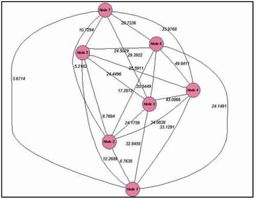
In this step, an edge-weighted complete graph is constructed, where its vertices are IoT devices and the weight of each edge is the Euclidean distance between its devices. In each iteration, for each cluster, a weighted graph is constructed from alive nodes. Figure 1 shows a weighted graph for a cluster with 7 nodes.

Figure 1. A weighted graph for a cluster with 7 nodes.

Step 2. The construction of the MST

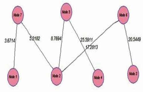
In this step, in each iteration, the MST is constructed for each weighted graph of previous step. If the number of alive nodes in one cluster would be more than one, this is a tree with the least total weight of edges between the spanning trees of that graph. The prime algorithm (Prim 1957) is used for MST construction. Figure 2 shows the MST of Figure 1.

Figure 2. The MST of Figure 1.

Step 3. Calculating the fitness function and selecting the optimal CH

The third step consists of the CH selection. In the process of CH selection, the fitness value for all candidates is calculated and based on it, the best CH is selected. We have considered all essential characteristics that a CH should have and combine them in a feature using a fitness function. In the following, first essential parameters are described and then the fitness function is defined.

Essential Parameters in Selecting a CH

The proposed algorithm belongs to the second category of CH selection algorithms, where in the first phase, the clustering is done and in the second phase, the CH is selected. After clustering, each node belongs to a cluster. In the second phase, each node is a CH candidate. For each CH candidate, the essential parameters that should be considered in evaluating its fitness are shown in Table 2.

Table 2. The essential parameters that are used in evaluating each candidate fitness

Parameter	Notation
The remaining energy of node $i$	$E_i$
The cluster that node $i$ belong to it	$C_i$
The number of alive nodes that belong to $C_i$	$N_i$
Total energy of other alive nodes that belong to $C_i$	$\sum _{j=1}^{N_i}{E}_j$
The distance of node $i$ to each node such as $j$ that is neighbor of it in MST	$d_{i{j}_{MST}}$
Total distances of node $i$ to all alive neighbor nodes in the minimum spanning tree	$\sum _{j=1}^{N_i}{d}_{i{j}_{MST}}$
The distance between two nodes $i$ and $j$ that belong to the same cluster	$d_{ij}$
Distance of node $i$ to the base station	$d_{iB}$
The number of alive neighbors of node $i$ in the MST	$N_{iMST}$

After the calculation of these parameters, the fitness value of each node to be a CH is calculated using equation 1(1) $F(i)=E_i\sum _{j=1}^{N_i}{E}_j\times \{\sum _{j=1}^{N_i}{d}_{i{j}_{MST}}\sum _{j=1}^{N_i}{d}_{ij}\times d_{iB}\times N_{iMST}{N}_i.$(1) ,

(1) $F(i)=E_i\sum _{j=1}^{N_i}{E}_j\times \{\sum _{j=1}^{N_i}{d}_{i{j}_{MST}}\sum _{j=1}^{N_i}{d}_{ij}\times d_{iB}\times N_{iMST}{N}_i.$(1)

Each node with a fitness value being more than other nodes of the same cluster is selected as the CH for that cluster. Thus, a node that its distance to the base station and total distance of it to other alive nodes that are neighbor of it in MST are minimum, and also the remaining energy of it and the number of its neighbors in MST are maximum, is the best selection to be a CH. The value of the fitness function is calculated for all sensor nodes and the node is qualified to be CH in the current round, for which this value is the highest.

Step 4. Data transferring

In this phase, all nodes that belong to a cluster transfer their data to their respective CH and the CH will then send the received data to the BS. Since the MST is constructed in each cluster, this tree is used to transfer data to the CH in addition to selecting the optimal CH. Instead of sending each node’s information directly to its CH, it transfers them to the parent in the MST and the data are transmitted in the hierarchical of MST to reach the corresponding CH. When the CH receives all corresponding data, it eventually transfers the collected data to the base station. It is also possible to have a multihop communication in each cluster and single-hop communication between CHs and the base station. Figure 3 shows the apparent appearance of the MST formed between the nodes of each cluster. To illustrate this, each cluster is shown with a special color and the CHs are represented with a larger symbol than the cluster member nodes (see Figure 3).

Figure 3. The constructed MST for all clusters.

Figure 4

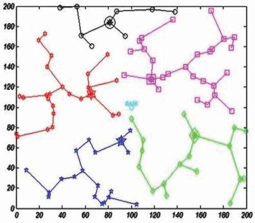
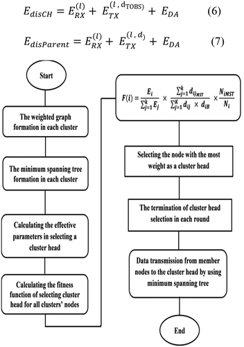
Figure 4. Flowchart of the EEMST algorithm.

Updating the Energy Level of the Nodes

Due to the fact that sending and receiving the data increase the consumption of node energy, the energy consumed per device should be estimated and remaining energy level of devices should be updated accordingly. In this paper, the energy model in Lee and Cheng 2012 is used, but due to using the MST to send data from member nodes to the CH in each cluster, it is necessary to revise the energy model of member nodes. Indeed, in addition to the CH, each member node receives data from other nodes too. Thus, the lost energy of the member nodes and CH is calculated using equation 2(2) $E_{TX}^{(l,\mathrm{d})}=\left\{\begin{array}{ccc}l\ast & E_{elec}^{TX}+l\ast {\epsilon }_{fs}\ast d^2& ,d_0{d}_0\\ l\ast & e_{elec}^{tx}+l\ast {\epsilon }_{mp}\ast =d^4& ,d\ge =d_0\end{array}\right.$(2) ,

(2) $E_{TX}^{(l,\mathrm{d})}=\left\{\begin{array}{ccc}l\ast & E_{elec}^{TX}+l\ast {\epsilon }_{fs}\ast d^2& ,d_0{d}_0\\ l\ast & e_{elec}^{tx}+l\ast {\epsilon }_{mp}\ast =d^4& ,d\ge =d_0\end{array}\right.$(2)

where $E_{TX}^{\left(\mathrm{l},d\right)}$ is the lost energy for the transmitter node, $d$ corresponds to the Euclidean distance of the transmitter and the receiver node in the MST, ${\mathrm{E}}_{\mathrm{e}\mathrm{l}\mathrm{e}\mathrm{c}}^{\mathrm{T}\mathrm{X}},{\epsilon }_{fs},{\epsilon }_{mp}$ and $d_0$ are constant values, which are being defined at the beginning of the network life, and $l$ is the length of packet in bits. The value of $l$ is constant and is determined in the beginning of the network life. The Euclidean distance between two nodes $\left(x_1,{\mathrm{y}}_1\right)$ and $\left(x_2,y_2\right)$ is calculated based on equation 3(3) $d=\sqrt{{(x_1-x_2)}^2+{(y_1-y_2)}^2}.$(3) ,

(3) $d=\sqrt{{(x_1-x_2)}^2+{(y_1-y_2)}^2}.$(3)

The lost energy value of the receiver node (parent, member node) is calculated based on the following equation:

(4) $E_{RX}^{(l)}=l\ast E_{elec}^{RX},$(4)

where $E_{elec}^{RX}$ is the fixed value that is defined at the beginning of the network life and $l$ is the packet length (bits) and is constant all over the network life. This is also being defined at the beginning. The amount of the lost energy of the CH node for receiving information from a node is also being calculated based on equation 4(4) $E_{RX}^{(l)}=l\ast E_{elec}^{RX},$(4) . The CH should then send the information to the base station, where it also consumes energy. To calculate this consumed energy value, equation 2(2) $E_{TX}^{(l,\mathrm{d})}=\left\{\begin{array}{ccc}l\ast & E_{elec}^{TX}+l\ast {\epsilon }_{fs}\ast d^2& ,d_0{d}_0\\ l\ast & e_{elec}^{tx}+l\ast {\epsilon }_{mp}\ast =d^4& ,d\ge =d_0\end{array}\right.$(2) is used, with a difference that d is the Euclidean distance between the CH and the base station. As shown in equation 5(5) $E_{RX}^{(NumberO{f}_{child})}=NumberO{f}_{child}\ast E_{elec}^{RX}.$(5) , due to the CH and receiver, node (parent) may have more than one child and the value of lost energy consumed for receiving information from all children should be multiplied by the number of children (node’s neighbors),

(5) $E_{RX}^{(NumberO{f}_{child})}=NumberO{f}_{child}\ast E_{elec}^{RX}.$(5)

Also, both the CH and the receiver node (parent) consumed some energy for data aggregation before transferring the data. This energy value is a constant and is denoted as E_DA. Accordingly, the lost energy for the CH and the receiver node (parent) is calculated based on the following equations:

(6) $E_{disCH}=E_{RX}^{(l)}+E_{TX}^{(l,{\mathrm{d}}_{\mathrm{T}\mathrm{O}\mathrm{B}\mathrm{S})}}+E_{DA},$(6)

(7) $E_{disParent}=E_{RX}^{(l)}+E_{TX}^{(l,d_{)}}+E_{DA},$(7)

where $E_{RX}^{\left(l\right)}$is the amount of lost energy of the CH node for receiving information from a node, $E_{TX}^{(l,{\mathrm{d}}_{\mathrm{T}\mathrm{O}\mathrm{B}\mathrm{S})}}$ is the lost energy of the CH node for sending the information to the base station, $d$ is the Euclidean distance of the CH and the BS and ${\mathbf{E}}_{\mathbf{D}\mathbf{A}}$ is the energy for data aggregation. In equation 7(7) $E_{disParent}=E_{RX}^{(l)}+E_{TX}^{(l,d_{)}}+E_{DA},$(7) , $E_{RX}^{\left(l\right)}$ is the lost energy value of the receiver node, $E_{TX}^{(l,d_{)}}$ is the lost energy for the transmitter node, $d$ is the Euclidean distance of the transmitter and receiver nodes in the MST and ${\mathbf{E}}_{\mathbf{D}\mathbf{A}}$ is the data aggregation energy. If a CH would be the only alive node in the cluster, the energy for data collecting (E_DA) will not be deducted from its energy. Now, the energy level of the nodes should be updated as stated in the following, so that in the next rounds, this energy is to be used. Based on G. Wang, Wang, and Tao 2009, the remaining energy of each node at the end of each round will be equal to

(8) $E_{Res}=E-E_{dis}.$(8)

This will be finished, when all nodes are dead and the network will be down.

Performance Evaluation

For evaluating the proposed, we conduct several experiments. In the following, we first describe the simulation environment and tools. Then, we determine the assumptions and default values that have been used for the simulated network configuration. Later, the evaluation metrics are determined. Finally, the simulation results and comparison results are depicted.

Simulation Setup

The EEMST algorithm is implemented in MATLAB. In order to evaluate the network lifetime in different situations, it can be considered with the number of different clusters. Also, since the location of the base station has a significant impact on the network lifetime, different locations for establishment of the base station are considered. In order to ensure accuracy of the simulation, the results were obtained at each stage of 30 iterations and then averaging was performed.

Assumptions and Default Values

The initial assumption and configuration values of the simulated network are depicted in Table 2.

Performance Evaluation Parameters

For evaluating the performance of the proposed EEMST algorithm, following criteria are used:

1. Network lifetime

2. The remaining energy of the nodes

3. Total number of data packets that a BS receives

4. Total energy consumed by CHs.

Performance Evaluation in Terms of Network Lifetime

To evaluate our proposed method, first, we conducted several experiments to investigate the impact of the different network configuration in the EEMST algorithm on the network lifetime. In the first one, the base station coordinates were (100,100), initial energy was 2 J and network area was 200*200 (config 1). In this algorithm, we explored the impact of the number of clusters on the network lifetime. The results of this experiment are depicted in Table 3.

Table 3. Comparing the network lifetime of the EEMST algorithm for different numbers of clusters, (x_s,y_s) = (100,100) and E = 2 J (config. 1)

Number of clusters	Network lifetime	First node dead
5	6791.8	2254.867
10	7661.567	1986.933
15	8303.8	1782.4
20	8646.733	1686.533

In the second experiment, we repeated the previous configuration with a new configuration, where the base station coordinates were (200,200), the initial energy was 2 J and the network area was 200*200 (config 2). Table 4 depicts the results of this experiment.

Table 4. Comparing the network lifetime of the EEMST algorithm for different numbers of clusters, (x_s,y_s) = (200,200) and E = 2 J (config. 2)

Number of clusters	Network lifetime	First node dead
5	6279.333	1184.333
10	7141.6	695.6333
15	7588.633	448.1667
20	7914.467	356.6667

Tables 5 and 6 show the results of third and fourth experiments, respectively. In the third experiment, the coordinates of the base station were (275,200) (conFigure 3). These were (300,300) (config 4) in the fourth experiment. Another parameters were the same as the first experiment.

Table 5. Comparing the network lifetime of the EEMST algorithm for different numbers of clusters, (x_s,y_s) = (275,200) and E = 2 J (config. 3)

Number of clusters	Network lifetime	First node dead
5	5232.9	774.8333
10	5418.4	309.7333
15	5580.4	220.7
20	5490.433	158.3

Table 6. Comparing the network lifetime of the EEMST algorithm for different numbers of clusters, (x_s,y_s) = (300,300) and E = 2 J (config. 4)

Number of clusters	Network lifetime	First node dead
5	2558.8	337.7
10	2179.533	114.2333
15	1836.333	59.93333
20	1637.933	56.1

Table 7

Table 7. The initial assumptions of the algorithm

Variables	Parameters	Values
S	Network area	100 × 100 m^2 200 × 200 m^2 1000 × 1000 m^2
n	Number of nodes	100
(xs,ys)	Base Station coordinates	(50,50), (100,100), (200,200), (200,275), (300,300), (500,500)
C	Number of clusters	5, 10, 15, 20
l	Data package length	4000 bit
d0	Energy model threshold	$\cong$87.71
Eelec	Energy of electronics	50nJ/bit
EDA	Data aggregation energy	5nJ/bit
efs	Amplifier coefficient (d < d0)	10pJ/bit/m^2
eamp	Amplifier coefficient (d ≥ d0)	0.0013pJ/bit/m^4
E	Initial energy	2 J, 0.5 J, 0.6 J

As the results in Tables 3–6 approve that when a BS coordinate is considered in the center of a network area or at the edge of the area, any increase in the number of clusters results in the increased network lifetime. Indeed, when the number of clusters increases, the intracluster distance decreases and this leads to the reduction in the energy required for intracluster communications. However, in a network with a base station outside the sensors area, the lower number of clusters shows better performance. In this case, the intercluster communication decreases and therefore, the required energy also decreased. Therefore, among the examined locations, the network with the BS in the center is better than the BS on the edge or outside of the sensors area. Indeed, if the BS is located in the center, required energy for sending messages to the BS is being decreased.

We compared our proposed algorithm (EEMST) with three baseline papers. These algorithms were LEACH (Heinzelman, Chandrakasan, and Balakrishnan 2000), Naïve Bayes (Jafarizadeh, Keshavarzi, and Derikvand 2017), BASA-WMST (Saravanan and Madheswaran 2014) and Hybrid algorithm (Praveen Kumar and Rajasekhara Babu 2019a). The results of this comparison are depicted in Figures 5 to 12.

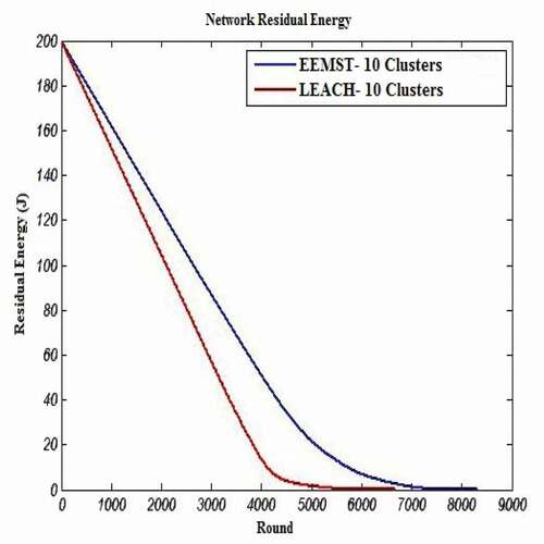
Figure 5. Comparing the network lifetime of EEMST and LEACH algorithms for C = 10, S = 200 × 200, (x_s,y_s) = (100,100) and E = 2 J (config. 5).

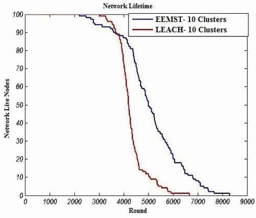
Figure 5 shows the results of comparison between EEMST and the LEACH algorithms with the term of network’s lifetime in the stated configuration. As is shown in this figure, the network’s lifetime in the proposed algorithm has significantly improved compared to the LEACH algorithm. Indeed, in EEMST, the CH is selected such that the energy of nodes is consumed uniformly. This lead to the increase in the lifetime of the network, while in the LEACH algorithm, CH is randomly selected. This results in unbalance energy consumption of CHs and reducing lifetime of the network.

As is seen in Figure 6, the EEMST algorithm outperforms the Naïve Bayes algorithm in terms of network lifetime, since the Naïve Bayes algorithm only considers residual energy and total distance of all member nodes to the cluster head, while our proposed algorithm considers other properties such as the number of alive nodes in each cluster and sum of remaining energies of other clusters’ nodes. Also, Figure 7 shows that our proposed algorithm has better performance than the BASA-WMST algorithm, since in each cluster, the communication is multihop and each node sends its data to the neighbor in MST. Thus, all nodes involve in data transmission and the CH consumes lower energy. Also, in selection of CH essential characteristics such as node energy, the distance of the node from other nodes and the location of node in MST are considered. Also, Figure 8 presents the network lifetime of our proposed algorithm compared with the BASA-WMST algorithm. Our approach outperforms the BASA-WMST algorithm since our approach is multihop and balances energy consumption between all nodes, while BASA-WMST is single-hop and energy consumption patterns of its nodes are not the same.

Figure 6. Comparing the network lifetime of EEMST and Naïve Bayes algorithms for C = 10, S = 100 × 100, (x_s,y_s) = (50,50) and E = 2 J (config. 6).

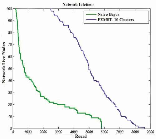
Figure 7. Comparing the network lifetime of EEMST and BASA-WMST algorithms for C = 10, S = 1000 × 1000, (x_s,y_s) = (500,500) and E = 0.6 J (config. 7).

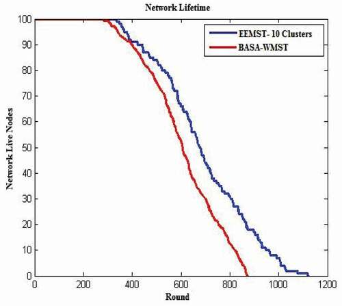
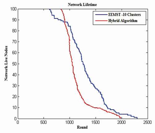
Figure 8. Comparing the network lifetime of EEMST and hybrid algorithm for C = 10, S = 100 × 100, (x_s,y_s) = (50,50) and E = 0.5 J (config. 8).

The Performance Evaluation in Terms of Energy

Figure 9 shows the comparison results of the EEMST algorithm with the LEACH algorithm in terms of remaining energy. This comparison shows that the EEMST algorithm outperforms the LEACH algorithm in terms of energy consuming. Indeed, in the proposed algorithm, it has been tried to have energy consumption balanced between all nodes of each cluster and thus, CHs and other nodes are more alive.

Figure 9. Comparing the remaining energy of the network nodes in the EEMST algorithm and LEACH algorithm for C = 10, S = 200 × 200, (x_s,y_s) = (100,100) and E = 2 J (config. 9).

Performance Evaluation for the Amount of Received Data Packets by the BS

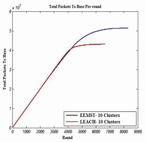
Figure 10 shows the total number of received packets at the BS in each round. As it has been shown in this figure, the total number of received packets in EEMST is more than that in the LEACH algorithm, since the proposed algorithm is multihop and each node sends data to its neighbor in MST. Indeed, by applying the multi-hop mechanism, the energy consumption pattern of all nodes in the network is similar, which leads to robustness in our network.

Figure 10. Comparing the total number of received data packets at the BS in the EEMST algorithm and LEACH algorithm for C = 10, S = 200 × 200, (x_s,y_s) = (100,100) and E = 2 J (config. 10).

The next evaluation results of the EEMST algorithm performance for the number of received data packets by the BS are shown in Figure 11. As is seen in this figure, the proposed algorithm outperforms other algorithms in terms of the total number of received packets by the BS.

Figure 11. Comparing the number of data packets received at different locations of the base station in the EEMST algorithm and LEACH for C = 5 and C = 10, S = 200 × 200, (x_s,y_s) = (100,100) and E = 2 J (config. 11).

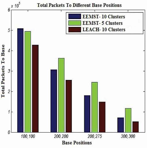
The previous depicted figures show that the number of received packets by the BS is dependent on the coordinates of BS and the number of clusters. As the base station moves farther from the network area, the fewer number of packets will be received in the BS. Also, at farther distances, the network with a fewer number of clusters has better performance than the network with more clusters. Therefore, according to the results, the network with more clusters and the location of the BS in the 100, 100 (center of the network area) will received the most data packets.

Performance Evaluation for Energy Consumption of CHs

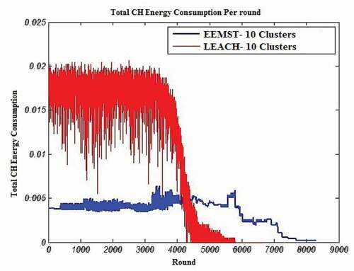
Figure 12 shows the comparison of total energy consumption by CHs in the EEMST algorithm and comparison of it with the LEACH algorithm. As it is shown in this figure, CHs in the EEMST algorithm in different rounds use less energy than LEACH algorithm CHs. The optimal selection of CH and intracluster multihop communication has two resons for this matter. Indeed, since nodes of each cluster transfer their data to their nearest neighbor’s node (parent) in the MST and the data are transmitted node to node to reach the corresponding CH, the CH consumes less energy for receiving and collecting data than intracluster single-hop mode.

Figure 12. Comparing the total energy consumption of CHs in the EEMST algorithm and the LEACH algorithm for C = 10, S = 200 × 200, (x_s,y_s) = (100,100) and E = 2 J (config. 12).

Conclusions

To maximize energy efficiency and thereby increase the lifespan of the IoT network, we studied optimal CH selection in this paper. By utilizing weighted graphs and Euclidean distance-based MST, we optimized the data routing between the CHs and the member nodes. It should be noted that specific criteria were taken into account during the selection process. The criteria include a node’s remaining energy, its distance to the base station, its number of neighbors in the MST and the total distances between the candidate node and its alive neighbors in the MST. Node criteria such as the number of neighbor nodes within the MST and the distances between the neighbor nodes ensure that each node communicates with the closest neighbor node within the MST. Energy is being saved in this case because intracluster communication is being reduced. The energy required for intercluster communications is reduced as well by selecting the closest CH to the base BS based on the node distance to the base station. The proposed algorithm applies multihop communications in each cluster single-hop communication between CHs and the base station. The experimental results demonstrated that using the weighted minimum spanning tree for routing and cluster head selection led to balancing energy consumption between all nodes and consequently increasing network lifetime.

Future Works

As a future work, we plan to improve the accuracy of our selection by incorporating more accurate weights. This can be achieved by the probability aspect for nodes or selecting CHs. Furthermore, we plan to use hierarchical optimization of graph geometry in order to reduce energy consumption.

Disclosure Statement

No potential conflict of interest was reported by the author(s).

References

- Afshoon, M., A. Keshavazi, T. Derikvand, and M. Bohlouli. 2020. Efficient Cluster Head Selection Using the Non-linear Programming Method for Wireless Sensor Networks. In: Bohlouli M., Sadeghi Bigham B., Narimani Z., Vasighi M., Ansari E. (eds) Data Science: From Research to Application. CiDaS 2019. Lecture Notes on Data Engineering and Communications Technologies, vol 45. Springer, Cham. doi:https://doi.org/10.1007/978-3-030-37309-2_1.
- Azad, P., Navimipour, N.J., Rahmani, A.M. et al. 2020. The role of structured and unstructured data managing mechanisms in the Internet of things. Cluster Comput 23: 1185–1198. doi:https://doi.org/10.1007/s10586-019-02986-2.
- Barolli, L., Q. Wang, E. Kulla, B. Kamo, F. Xhafa, and M. Younas. 2012. “A Fuzzy-Based Simulation System for Cluster-Head Selection and Sensor Speed Control in Wireless Sensor Networks,” 2012 Third International Conference on Emerging Intelligent Data and Web Technologies, pp. 16-22, doi: https://doi.org/10.1109/EIDWT.2012.14.
- Behera, T. M., S. K. Mohapatra, U. C. Samal, M. S. Khan, M. Daneshmand, and A. H. Gandomi. 2019. Residual Energy Based Cluster-Head Selection in WSNs for IoT Application. IEEE INTERNET OF THINGS JOURNAL 6 (3):5132–39. doi:https://doi.org/10.1109/JIOT.2019.2897119.
- Busch, C., R. Kannan, and A. V. Vasilakos. 2012. Approximating congestion+ dilation in networks via” quality of routing” games. IEEE Transactions on Computers 61 (9):1270–83. doi:https://doi.org/10.1109/TC.2011.145.
- Cao, X., H. Zhang, J. Shi, and G. Cui. 2008. “Cluster Heads Election Analysis for Multi-hop Wireless Sensor Networks Based on Weighted Graph and Particle Swarm Optimization,” 2008 Fourth International Conference on Natural Computation, pp. 599-603, doi: https://doi.org/10.1109/ICNC.2008.693.
- Chapuis, G., H. Djidjev, D. Lavenier, and R. Andonov. 2017. “GPU-accelerated shortest paths computations for planar graphs.
- Chen, F., P. Deng, J. Wan, D. Zhang, A. V. Vasilakos, and X. Rong. 2015. Data mining for the internet of things: literature review and challenges. International Journal of Distributed Sensor Networks 11 (8):431047. https://www.hindawi.com/journals/ijdsn/aa/431047/abs/.
- Chen, J., and H. Shen. 2008. MELEACH-L: More energy-efficient LEACH for large-scale WSNs. 4th International Conference on Wireless Communications, Networking and Mobile Computing (Wicom) 1–4.
- Chiu, S. L. 1994. Fuzzy model identification based on cluster estimation. Journal of Intelligent & Fuzzy Systems 2 (3):267–78. doi:https://doi.org/10.3233/IFS-1994-2306.
- Du, X., M. Guizani, Y. Xiao, and H.-H. Chen. 2007. Two tier secure routing protocol for heterogeneous sensor networks. IEEE Transaction on Wireless Communications 6 (9):3395–401. doi:https://doi.org/10.1109/TWC.2007.06095.
- Elias, K., P. Mohanty Saraju, C. Gavin, A. Umar, and S. Prabha. 2016. Design of a high-performance system for secure image communication in the internet of things. IEEE 4:1222–42.
- Gajjar, S., M. Sarkar, and K. Dasgupta. 2014. Cluster head selection protocol using Fuzzy logic for wireless sensor networks. International Journal of Computer Applications 97 (7):38–43. http://search.proquest.com/openview/3d2a3ffe9d4931fe2b42dc435d0e670e/1?pq-origsite=gscholar&cbl=136216.
- Han, K., J. Luo, Y. Liu, and A. V. Vasilakos. 2013. Algorithm design for data communications in duty-cycled wireless sensor networks: A survey. IEEE 51 (7):107–13.
- Han, T., L. Zhang, S. Pirbhulal, W. Wanqing, and C. D. A. Victor Hugo. 2019. A novel cluster head selection technique for edge-computing based IoMT systems. Computer Networks 158:114–22. doi:https://doi.org/10.1016/j.comnet.2019.04.021.
- Heinzelman, W. R., A. Chandrakasan, and H. Balakrishnan. 2000. “Energy-efficient communication protocol for wireless microsensor networks,” Proceedings of the 33rd Annual Hawaii International Conference on System Sciences, pp. 10 pp. vol.2, doi: https://doi.org/10.1109/HICSS.2000.926982.
- Hu, W., W. Yao, H. Yawei, and L. Huanhao. 2019. Selection of cluster heads for wireless sensor network in Ubiquitous power internet of things. International Journal of Computers Communications & Control 14 (3):344–58. doi:https://doi.org/10.15837/ijccc.2019.3.3573.
- Huang, G., L. Xiaowei, and H. Jing 2006. “Dynamic Minimal Spanning Tree Routing Protocol for Large Wireless Sensor Networks,” 2006 1ST IEEE Conference on Industrial Electronics and Applications, pp. 1-5, doi: https://doi.org/10.1109/ICIEA.2006.257220.
- Hussain, S., and O. Islam. 2007. “An Energy Efficient Spanning Tree Based Multi-Hop Routing in Wireless Sensor Networks,“ 2007 IEEE Wireless Communications and Networking Conference, pp. 4383-4388, doi: https://doi.org/10.1109/WCNC.2007.799.
- Jafarizadeh, V., A. Keshavarzi, and T. Derikvand. 2017. Efficient cluster head selection using Naïve Bayes classifier for wireless sensor networks. Wireless Netw 23: 779–785. doi:https://doi.org/10.1007/s11276-015-1169-8.
- Jing, Q., A. V. Vasilakos, J. Wan, L. Jingwei, and D. Qiu. 2014. Security of the internet of things: Perspectives and challenges. Wireless Networks 20 (8):2481–501. doi:https://doi.org/10.1007/s11276-014-0761-7.
- Keshavarzi, A., A. T. Haghighat, and M. Bohlouli. 2017. Adaptive resource management and provisioning in the cloud computing: A survey of definitions, standards and research roadmaps. KSII Transactions on Internet and Information Systems (TIIS) 11 (9):4280–300.
- Keshavarzi, A., A. T. Haghighat, and M. Bohlouli. 2020. Enhanced time-aware QoS prediction in multi-cloud: A hybrid k-medoids and lazy learning approach (QoPC). Computing 102 (4):923–49. doi:https://doi.org/10.1007/s00607-019-00747-y.
- Keshavarzi, A., A. T. Haghighat, and M. Bohlouli. 2021. Clustering of large scale QoS time series data in federated clouds using improved variable Chromosome Length Genetic Algorithm (CQGA). Expert Systems with Applications 164:113840. doi:https://doi.org/10.1016/j.eswa.2020.113840.
- Lachowski, R., M. E. Pellenz, E. Jamhour, M. C. Penna, and R. Souza. 2015. An efficient distributed algorithm for constructing spanning trees in wireless sensor networks. Sensors 15: 1518–36. OPEN ACCESS. doi:https://doi.org/10.3390/s150101518.
- Lee, J.-S., and W.-L. Cheng. 2012. Fuzzy-logic-based clustering approach for wireless sensor networks using energy predication. IEEE Sensors Journal 12 (9):2891–97. doi:https://doi.org/10.1109/JSEN.2012.2204737.
- Li, C., H. Zhang, B. Hao, and L. Jiandong. 2011. A survey on routing protocols for large-scale wireless sensor networks. Sensors 11:3498–526. doi:https://doi.org/10.3390/s110403498.
- Li, M., L. Zhenjiang, and A. V. Vasilakos. 2013. A survey on topology control in wireless sensor networks: Taxonomy, comparative study, and open issues. IEEE 101 (12):2538–57. doi:https://doi.org/10.1109/JPROC.2013.2257631.
- Lindsey, S., and C. S. Raghavendra. 2002. “PEGASIS: Power-efficient gathering in sensor information systems,” Proceedings, IEEE Aerospace Conference, pp. 3-3, doi:https://doi.org/10.1109/AERO.2002.1035242.
- Liu, X.-Y., Y. Zhu, L. Kong, C. Liu, Y. Gu, A. V. Vasilakos, and M.-Y. Wu. 2015. CDC: Compressive data collection for wireless sensor networks. IEEE Transactions on Parallel and Distributed Systems 26 (8):2188–97. doi:https://doi.org/10.1109/TPDS.2014.2345257.
- Meng, T., W. Fan, Z. Yang, G. Chen, and A. V. Vasilakos. 2016. Spatial reusability-aware routing in multi-hop wireless networks. IEEE Transactions on Computers 65 (1):244–55. doi:https://doi.org/10.1109/TC.2015.2417543.
- Muruganathan, S. D., D. C. F. Ma, R. I. Bhasin, and A. O. Fapojuwo. 2005. A centralized energy-efficient routing protocol for wireless sensor networks. IEEE Communications Magazine 43 (3):8–13. doi:https://doi.org/10.1109/MCOM.2005.1404592.
- Nguyen, H. P., L. Phan Quang Huy, P. Van Viet, N. Xuan Phuong, D. Balasubramaniam, and A.-T. Hoang. 2021. Application of the Internet of Things in 3E (efficiency, economy, and environment) factor-based energy management as smart and sustainable strategy. Energy Sources, Part A: Recovery, Utilization, and Environmental Effects 1–23. doi:https://doi.org/10.1080/15567036.2021.1954110.
- Ni, Q., Q. Pan, D. Huimin, C. Cao, and Y. Zhai. 2015. A novel cluster head selection algorithm based on fuzzy clustering and particle swarm optimization. IEEE/ACM Transactions on Computational Biology and Bioinformatics 14 (1):76–84. doi:https://doi.org/10.1109/TCBB.2015.2446475.
- Ozdemir, S., and Y. Xiao. 2009. Secure data aggregation in wireless sensor networks: A comprehensive overview. Computer Networks 53 (12):2022–37. doi:https://doi.org/10.1016/j.comnet.2009.02.023.
- Pal, V., G. Singh, R. P. Yadav, and R. P. Yadav. 2015. Cluster head selection optimization based on genetic algorithm to prolong lifetime of wireless sensor networks. Procedia Computer Science 57:1417–23. doi:https://doi.org/10.1016/j.procs.2015.07.461.
- Peyravi, F., and A. Keshavarzi. 2009.“Agent Based Model for Call Centers Using Knowledge Management,” 2009 Third Asia International Conference on Modelling & Simulation, pp. 51-56, doi:https://doi.org/10.1109/AMS.2009.147.
- Pourghebleh, B., Hayyolalam, V. A 2020. comprehensive and systematic review of the load balancing mechanisms in the Internet of Things. Cluster Comput 23: 641–661. doi:https://doi.org/10.1007/s10586-019-02950-0
- Praveen Kumar, R. M., and M. Rajasekhara Babu. 2019. “Implementing self adaptiveness in whale optimization for cluster head section in internet of things.” Cluster Computing 22 (1):1361–72. doi:https://doi.org/10.1007/s10586-017-1628-3
- Praveen Kumar, R. M., and M. Rajasekhara Babu. 2019a. A hybrid cluster head selection model for internet of things. Cluster Computing 22 (6):13095–107. doi:https://doi.org/10.1007/s10586-017-1261-1.
- Prim, R. C. 1957. Shortest connection networks and some generalizations. Bell Labs Technical Journal 36 (6):1389–401. doi:https://doi.org/10.1002/j.1538-7305.1957.tb01515.x.
- Saravanan, M., and M. Madheswaran. 2014. A hybrid optimized weighted minimum spanning tree for the shortest intrapath selection in wireless sensor network. Mathematical Problems in Engineering: 2014. https://www.hindawi.com/journals/mpe/2014/713427/abs/
- Sharma, T., B. Kumar, G. S. Tomar, and I. Berry. 2014. Particle swarm optimization based cluster head election approach for wireless sensor network. International Journal of Smart Device and Appliance 2 (2):11–26. http://iacsportal.org/images/demo/ijsda/2014/IJSDA_2014_2_2_article2.pdf.
- Varghese, B. 2016. Cluster head selection in wireless sensor networks. International Journal of Latest Research in Engineering and Technology (IJLRET) 2 (4):60–66.
- Vo, D. T., X. P. Nguyen, N. Thai Duong, H. Rahmat, H. Thanh Tung, and D. T. Nguyen. 2021. A review on the internet of thing (IoT) technologies in controlling ocean environment. Energy Sources, Part A: Recovery, Utilization, and Environmental Effects 1–19. doi:https://doi.org/10.1080/15567036.2021.1960932.
- Wang, G., Y. Wang, and X. Tao. 2009. “An Ant Colony Clustering Routing Algorithm for Wireless Sensor Networks,” 2009 Third International Conference on Genetic and Evolutionary Computing, pp. 670-673, doi:https://doi.org/10.1109/WGEC.2009.22.
- Wang, W., B. Wang, Z. Liu, L. Guo, and W. Xiong. 2011. A cluster-based and tree-based power efficient data collection and aggregation protocol for wireless sensor networks. Information Technology Journal 10 (3):557–64. doi:https://doi.org/10.3923/itj.2011.557.564.
- Wang, X., and H. Qian. 2012. Constructing a 6LoWPAN wireless sensor network based on a cluster tree. IEEE Transactions on Vehicular Technology 61 (3):1398–405. doi:https://doi.org/10.1109/TVT.2012.2185260.
- Xu, X., R. Ansari, A. Khokhar, and A. V. Vasilakos. 2015. Hierarchical Data Aggregation Using Compressive Sensing (HDACS) in WSNs. ACM Transactions on Sensor Networks (TOSN) 11 (3):45. doi:https://doi.org/10.1145/2700264.
- Younis, O., and S. Fahmy. 2004. HEED: A hybrid, energy-efficient, distributed clustering approach for Ad Hoc sensor networks. IEEE Transactions on Mobile Computing 3 (4):366–79. doi:https://doi.org/10.1109/TMC.2004.41.
- Zeng, Y., K. Xiang, L. Deshi, and A. V. Vasilakos. 2013. Directional routing and scheduling for green vehicular delay tolerant networks. Wireless Networks 19 (2):161–73. doi:https://doi.org/10.1007/s11276-012-0457-9.
- Zhang, J., Y. Xie, D. Liu, and Z. Zhang. 2012. OCTBR: Optimized Clustering Tree Based Routing Protocol for Wireless Sensor Networks.
- Zhang, X. M., Y. Zhang, F. Yan, and A. V. Vasilakos. 2015. Interference-based topology control algorithm for delay-constrained mobile Ad Hoc networks. IEEE Transactions on Mobile Computing 14 (4):742–54. doi:https://doi.org/10.1109/TMC.2014.2331966.
- Zheng, G., and H. Zhengbing. 2010. Tree routing protocol with location-based uniformly clustering strategy in WSNs. Special Issue: All-Optically Routed Networks Guest Editors: Antonio Teixeira, Anna Tzanakaki, Davide Careglio, and Miroslaw Klinkowski 5 (11):1243–388. doi:https://doi.org/10.4304/jnw.5.11.1245-1247.
- Zhou, B., A. Marshall, and L. Th. 2005. “An energy-aware virtual backbone tree for wireless sensor networks,” GLOBECOM '05. IEEE Global Telecommunications Conference, 2005., pp. 6 pp.-, doi:https://doi.org/10.1109/GLOCOM.2005.1577373.