Artificial Bee Colony-Artificial Neural Network (ABC-ANN) Hybrid Algorithm’s Performance on the Modeling of Thermodynamic Properties of a Refrigerant Gas (R404a)

ABSTRACT

In this study, it was aimed to determine the thermodynamic properties of an environmentally friendly refrigerant (R404a) for both the saturated liquid–vapor region (wet vapor) and superheated vapor region, in the temperature range of 173–498°K, and the pressure range of 10–3600 kPa by using an adaptive artificial neural network algorithm. Performing the analysis of these gases with differential equations by using a computer is very time consuming and requires high computational power for calculation. Using numerical equations for modeling the thermodynamic properties of gasses to eliminate these drawbacks is a more accurate approach and this modeling can be accomplished with artificial intelligence algorithms such as the Artificial Neural Network (ANN). The proper selection of the activation function, which is one of the most important parameters for ANN, directly affects the validity of the model according to the problem and its application. In this study, an adaptive ANN was developed in which the optimal activation function combination was found by using the ABC algorithm and thus the error of the network were reduced when compared to the classical ANN. The improvements of in percentage errors were observed to increase from 7.55% to 76.68%. Finally, the accuracy of the numerical equations that describe the thermodynamic properties of R404a gas was increased. Using this technique helps to figure out the performance of the gas under related working conditions.

Introduction

Modeling the thermodynamic behavior of a gas, depending on various parameters such as temperature, pressure, and volume, is one of the critical issues. The enthalpy and entropy values of the gas, under the predetermined operating conditions, are obtained from the H-S graph or the Mollier diagram. It is very effective to use modeling methods such as artificial neural networks in obtaining these values, which are very difficult to express mathematically for the wet or the super-heated region. Additionally, modeling is always used before any experimental testing to formulate new blends or to study the effect of changes in the composition, on the behavior and cooling performance (Doubek 2018).

Although Artificial Neural Network (ANN) has successfully calculated satisfied results in solving nonlinear equations, it is difficult to find the minimum global point if the model is not fully determined. In this aspect, the most important factor is to determine the activation function depending on the model. Another disadvantage is the need for a huge and consummate data set for developing an effective model with high estimation accuracy. Avoiding these disadvantages can be achieved with a hybrid algorithm that selects the most appropriate activation function of the ANN with a meta-heuristic algorithm. This feature takes an advantage over hybrid methods against classical AI-based methods. Hybrid algorithm-based optimization and estimation models are suitable for all branches of science. Furthermore, it provides great ease in predicting data where experimental applications are difficult to conduct. In addition, hybrid algorithms obtain more accurate and faster solutions for the optimization of nonlinear systems (Sonmez et al. 2015).

In this study, the thermodynamic properties of a refrigerant gas were determined by utilizing an adaptive/hybrid algorithm. Studies have been carried out on many different refrigerants and various efforts are underway to find new gases that are more efficient, energy-efficient, affordable, and environmentally friendly. It is important to test these refrigerants and figure out their thermodynamic properties. The R404a has been selected for calculating its thermodynamic properties by using a hybrid algorithm. R404A is a mixture of R-125 (44%), R-143a (52%), and R134a (4%). It is a non-ozone-depleting, long-term alternative to R-502 and R-22, as these gasses are well suited for low- and medium-temperature refrigeration applications. Its chemical notation is CHF2CF3/CH3CF3/CH2FCF3, its molecular weight is 97.60, and boiling point at one atmosphere is – 46.45°C.

The most common algorithms for defining the parameters of refrigerant gases are ANN or GA. Sozen et al. proposed an approach by using ANN to determine the thermodynamic properties of the R404a gas. They examined and compared the performance of different ANN algorithms and the number of hidden layers (Sözen, Arcaklioğlu, and Menlik 2010). In another study, ANNs with a back-propagation algorithm were employed in different gases in order to obtain the accurate prediction models for the thermodynamic properties. ANNs show their ability to accurately predict the properties of refrigerants (Mora R et al. 2014). In another ANN modeling of the refrigerant, thermodynamic performance was realized under a variable speed compressor. Hence, this method avoids the need for a large number of experiments to analyze of the system (Kizilkan 2011).

Mohebbi et al. developed a new approach to predict the density of a liquid for different refrigerants by using a neural network based on a genetic algorithm (GA). The main prediction was realized by ANN; moreover, some parameters such as the number of hidden processing elements, the learning rate and the momentum rate were optimized by the GA (Mohebbi, Taheri, and Soltani 2008). The Sencan et al. proposed an artificial neural network (ANN) model to determine properties such as the heat conduction coefficient, dynamic viscosity, kinematic viscosity, thermal diffusivity, density, and the specific heat capacity of refrigerants (Şencan, Köse, and Selbaş 2011).

The reason for using ANN in studies is its strong modeling capability. When ANN is not preferred, different equations have been developed, similar to the work performed by Zyczkowski et al., to obtain the properties of the R1234 gas (Zyczkowski et al. 2020). The use of cubic equations of state, which is another modeling technique, is highly preferred in the literature. A desktop application was developed to model the thermophysical properties of the two different types of refrigerants, namely R1234yf and R410A (Atalay and Coban 2015). Another cubic equation of state modeling study was conducted to generate thermodynamic property data (Neto and Barbosa 2010). A three-parameter cubic equation of state was developed by Coquelet et al. to predict the properties of mixture gases (Coquelet, El Abbadi, and Houriez 2016). Sahin et al. preferred gene expression programming to estimate the thermodynamic properties of the R513A refrigerant (Sahin, Kovacı, and Dikmen 2021).

In this study, a proposed hybrid algorithm was developed and applied to predict the thermodynamic properties (enthalpy and entropy) of the R404a gas. The key point is finding the enthalpy and entropy value of the gas under specified conditions. Probably, the easiest and fastest way to achieve this value is to model mathematically. Here, the modeling capability of ANN becomes crucial. On the other hand, the optimum selection of the parameters of the ANN affects the performance of the model considerably. In this study, a new hybrid algorithm was proposed by combining ANN with an Artificial Bee Colony (ABC). The ABC was used for selecting the best suitable activation function of ANN. The results show that a hybrid ANN produces better results as compared to a classical ANN. Furthermore, compared with previous studies, the error of modeling has been reduced and the modeling capacity of ANN has been increased with hybrid algorithms.

This manuscript is organized into four sections. The second section includes the mathematical definitions of the algorithms (classical ANN, ABC and adaptive algorithm). In the last subsection of this section, the methodology, equations, and combining of the steps of ANN and ABC are represented. The third section includes applications of the proposed hybrid algorithm for modeling the thermodynamic properties. The experimental results of modeling for the enthalpy and entropy data of the R404a gas are given in the last section.

Modeling of the R404 Gas by an Adaptive Artificial Neural Network (AANN)

Classical ANN

ANN is one of the most powerful methods in many processes such as pattern recognition, classification, function estimation, and optimization. Many successful applications of these processes have been developed thanks to the method that imitates the human nervous system and the brain’s learning ability. There are several network structures with different types of learning in ANN. Back propagation (BP) is the most common network structure and a powerful algorithm type for the node weights adjustment (Dursun and Ozden 2017; Mohanraj, Jayaraj, and Muraleedharan 2012).

As can be seen in the general network structure, which is given in Figure 1, a BP network structure consists of layers including an input layer, at least one hidden layer, and an output layer; and characteristics including a series of propagation errors (PEs), an activation function for each PE in layers, and weights. In order to realize the training process known as the generalized delta rule, in the beginning, random values are assigned to each weight and then input samples are delivered to the network in order. In this feed-forward process, outputs are calculated for each input sample. Then error signals are calculated by comparing the calculated outputs and targets. After this, these error signals are propagated backward from output to input layer in order to make weight adjustments. This feed forward-back propagation process repeats until the total error value reaches the expected minimum value and then the learning process is stopped (Ahmed et al. 2021; Efkolidis et al. 2019).

Figure 1. General structure of the BP Neural Network.

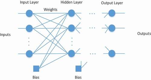
When it is assumed that A defines the input vector and B defines the desired target, A and B values in the network for n inputs and m outputs can be given as follows.

(1) $A=\left(a_1,a_2,\cdots \cdots ,a_n\right)$(1)

(2) $B=\left(b_1,b_2,\cdots \cdots ,b_n\right)$(2)

In the feed-forward process for training, a set of input samples is given to the input layer, and they move to the hidden layer through weights. Each PE in the hidden layer calculates the sum of its weighted inputs to calculate the net output. The net output of the i-th PE on j-th layer is calculated as follows.

(3) $ne{t}_i^j=\sum _{k=0}^n{w}_{ik}{a}_{ik}+b_k$(3)

Where w_ik is the weight value of i-th PE on k-th layer. Then the activation value is calculated as follows by subjecting it to an activation function. Transfer functions used in this study are given in Table 1.

(4) $b_{net}=f^k\left(ne{t}_i\right)$(4)

Table 1. Activation functions used in AANN

Function Number	Function Name	Function
1	Linear	$f\left(x\right)=w_{ik}{a}_{ik}+b_k$
2	Threshold	$f\left(x\right)=\left\{\begin{array}{ccc}1& if& w_{ik}{a}_{ik}+b_k\ge 0\\ 0& if& w_{ik}{a}_{ik}+b_k<0\end{array}\right.$
3	Logistic Sigmoid	$f\left(x\right)=\frac{1}{1+e^{w_{ik}{a}_{ik}+b_k}}$
4	Sinus	$f\left(x\right)=sin\left(w_{ik}{a}_{ik}+b_k\right)$
5	Hyperbolic Tangent	$f\left(x\right)=\frac{1-e^{-2\left(w_{ik}{a}_{ik}+b\right)}}{1+e^{-2\left(w_{ik}{a}_{ik}+b\right)}}$
6	Radial Bases	$f\left(x\right)=e^{-{\left(w_{ik}{a}_{ik}+b\right)}^2}$

These activation values are moved to the output layer and real outputs of the network are calculated in the same way. The BP networks aim to minimize the error between the desired output b and the real output of the network b_net. The network training is continued until this error value is at the minimum level.

Adaptive ANN

Unlike the classical ANN method, the AANN method has a heuristic search unit. AANN is achieved by optimizing ANN with ABC. It is important to note that the hybrid methods can be applied to several optimization problems (Awan et al. 2014; Karaboga and Ozturk 2011; Shah et al. 2012; Shunmugapriya and Kanmani 2017; Tsai 2014). The developed method is based on the hypothesis that neurons can respond to different characteristics. To realize this hypothesis, neurons in a network are designed to have different types of activation functions. The task of the heuristic search algorithm is to determine the type of function of each neuron to maximize the network performance. In this paper, Artificial Bee Colony (ABC) algorithm is used as a heuristic search unit. The six different transfer functions, which are used by each neuron in the network, are determined by the ABC algorithm. These functions have been presented in Table 1 above.

ABC Based Heuristic Search Unit

Artificial Bee Colony is a metaheuristic optimization algorithm and was initially defined by Karaboğa in 2005, and it imitates the life processes and attitudes of honeybees in a colony (Karaboga 2005). In the ABC algorithm, three types of artificial bees, which are namely: employed, onlookers, and scouts, are defined to find the food source with the highest nectar amount by modifying their food positions with time, in the search process. The duty of the employed bees is to exploit the food sources and giving information about the nectar amount to onlookers. The duty of onlookers is to wait at the dancing area and to select the food source. Scouts aim to discover new food sources. The numbers of employed and onlooker bees are half of the colony size, and this number corresponds to the solution number in the search space, because of assigning one employer bee for each food source (Karaboga and Akay 2009; Karaboga and Basturk 2007, 2008; Karaboga and Ozturk 2009; Ozturk and Karaboga 2011; Sonmez 2013).

Implementation of the ABC Algorithm for Optimizing ANN

In the ABC algorithm, the position of a food source corresponds to a possible solution to the problem. For this purpose, in this study, ABC creates a sequence of sources (a set of solution candidates) as the number of neurons in the AANN network model. Accordingly, for a network with n-pieces of neurons, the representation of m-number of solution candidates can be expressed as given in Eq. (5)(5) $S\equiv \left[\begin{array}{ccc}{g}_{11}& \cdots & g_{1n}\\ ⋮& \ddots & ⋮\\ g_{m1}& \dots & g_{mn}\end{array}\right],F\equiv \left[\begin{array}{c}{f}_1\\ ⋮\\ f_m\end{array}\right]$(5) .

(5) $S\equiv \left[\begin{array}{ccc}{g}_{11}& \cdots & g_{1n}\\ ⋮& \ddots & ⋮\\ g_{m1}& \dots & g_{mn}\end{array}\right],F\equiv \left[\begin{array}{c}{f}_1\\ ⋮\\ f_m\end{array}\right]$(5)

In Eq. (5(5) $S\equiv \left[\begin{array}{ccc}{g}_{11}& \cdots & g_{1n}\\ ⋮& \ddots & ⋮\\ g_{m1}& \dots & g_{mn}\end{array}\right],F\equiv \left[\begin{array}{c}{f}_1\\ ⋮\\ f_m\end{array}\right]$(5) ), each row in S is a solution candidate for the problem, and each row in F represents the fitness value of the corresponding solution candidate. The task of the ABC is to improve and update the solution candidates in the S-set and to record the candidate with the best fitness value as a solution. The pseudo-code and operation steps of the intuitive search unit are given in Algorithm 1. The flow chart of the adaptive ANN is presented in Figure 2.

Table

Algorithm 1. Pseudo-code of the ABC algorithm

Defining of cost function Determining of Colony size (p) Creation of Solution Candidate Set (S) (Initial Colony) Repeat 1:p Calculate fitness if (ending criteria) Save the best solution in S and exit else Move the employed bees onto their food sources and determine their nectar amounts. Move the onlookers onto the food sources and determine their nectar amounts. Move the scouts for searching new food sources. Memorize the best food source found so far end for

Figure 2. Flow chart of the proposed adaptive algorithm.

Classical ANN activation functions are defined at the beginning of the algorithm. As seen in Figure 2, the AANN starts with the random selection of activation functions for the neurons. The network is trained by the dataset and the performance of the network is evaluated by the RMSE value. Then this information is used in the ABC algorithm to update the activation functions. The main steps of ABC are applied to find the optimal function. This loop continues until the stopping criteria are satisfied. In this study, ABC aims to find the optimal combination of activation functions used by neurons, in the two hidden layers in the AANN network. In order to achieve this, the cost function used for optimization is defined as the Root Mean Square Error (RMSE) value produced by ANN for each epoch. ABC algorithm minimizes this error value by operating in each epoch during the learning process. Here, the implementations of the ABC algorithm for optimization are explained below step by step.

Step 1: Data input

In this step, the cost functions, which will be used in ANN and, given in Table 1 are defined.

Step 2: Initialization of ABC parameters

In this step, ABC parameters such as the colony dimension, maximum cycle number (MCN), number of variables, and limit parameters are set. The defined parameters of the ABC algorithm for minimizing the RMSE value are given in Table 2.

Table 2. Defined parameters for ABC algorithm

Colony dimension	40
MCN	400
Number of variables	10
Limit parameter	3000

Step 3: Creation of solution candidate set

In this step, a set of food sources (m -number of solution candidates for a network with n-pieces of neurons), which is given in Eq. (5(5) $S\equiv \left[\begin{array}{ccc}{g}_{11}& \cdots & g_{1n}\\ ⋮& \ddots & ⋮\\ g_{m1}& \dots & g_{mn}\end{array}\right],F\equiv \left[\begin{array}{c}{f}_1\\ ⋮\\ f_m\end{array}\right]$(5) ), is generated randomly.

Step 4: Calculation of fitness

Here, the fitness values for each food source positions are calculated by the RMSE value obtained from ANN. Then, the best fitness value is memorized.

Step 5: Move the employed bees onto their food sources and determine their nectar amounts

In this step, a food source position is modified by an employed bee. Thus, a new food source is created by visual information. Then, the nectar amount of this new source is calculated. Creating this new source is achieved by the following equation.

(6) $v_{ij}=g_{ij}+{\alpha }_{ij}\left(g_{ij}-g_{kj}\right),k\in (1,2,\dots ..,S),j\in (1,2,\dots ..,D)$(6)

where, k and j are indices chosen randomly, $\alpha$is a random number in the interval of $\left[-1,1\right]$, D is the number of parameters to be optimized. Then, a comparison between the fitness values of the old food source and the new one is conducted by the employed bees. If the new nectar amount is better than the old one, the new food source is memorized. Otherwise, the old food source is kept and the new one is discarded.

Step 6: Move the onlookers onto the food sources and determine their nectar amounts

After the previous step, employed bees come back to the hive to share information on the nectar amount of the sources. Then, according to this information, onlooker bees select a new food source and calculate its fitness value. The selection process is achieved by a probability value given as follows.

(7) $P_i=\frac{fitnes{s}_i}{\sum _{j=1}^{S}fitnes{s}_j}$(7)

Step 7: Move the scouts for searching new food sources

In this step, onlooker bees find new positions by modifying existing food source positions and then they calculate fitness values of the new sources. The evaluation and discarding process of food sources are conducted in the same way as given in step 5.

Step 8: Memorize the best food source found so far

The best food sources are kept memorized and the number of cycle is increased.

Step 9: Stopping the search process

This loop between steps 5 to 9 continues until the stopping criterion is met. The stop criterion is defined with the maximum cycle number (MCN).

Application of the Proposed Adaptive Model

The proposed adaptive model was developed for both the saturated liquid–vapor region (wet vapor, WV) and the superheated vapor (SHV) of R404a. The output parameters of the prediction models are thermodynamic properties such as enthalpy and entropy. The first model that has two inputs of “temperature” and “vapor quality” developed the R404a gas parameters under the wet vapor region. The second model that has three inputs of “temperature,” “pressure” and “volume” developed the R404a gas parameters under the superheated vapor region.

ANN and Adaptive AANN program codes have been developed and written in Visual Studio.Net by using C# language. The implementations of the algorithm and problem formulation have been conducted on the same platform. The algorithm is simulated on an Intel Core2 Duo processor with 2.2 GHz frequency and 2046 MB RAM.

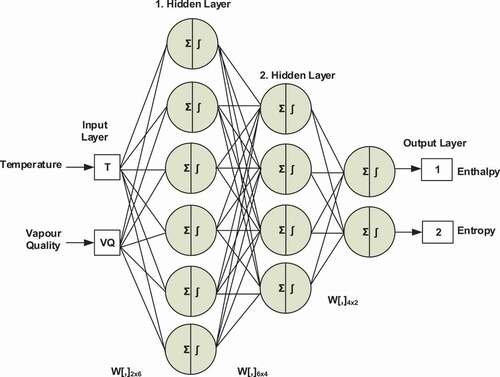
In Figure 3, the proposed AANN model for the WV region is given. It has three layers as two inputs, hidden layers, and outputs. The input parameters of the developed model are temperature and vapor quality. Enthalpy and entropy, which are the output parameters, represent the thermodynamic properties of the R404a. The outputs are applied to the model separately, since the data distribution has completely different characteristics. The first case shows enthalpy and the second one shows the entropy parameter of the gas.

Figure 3. The proposed model of the gas under wet vapor region.

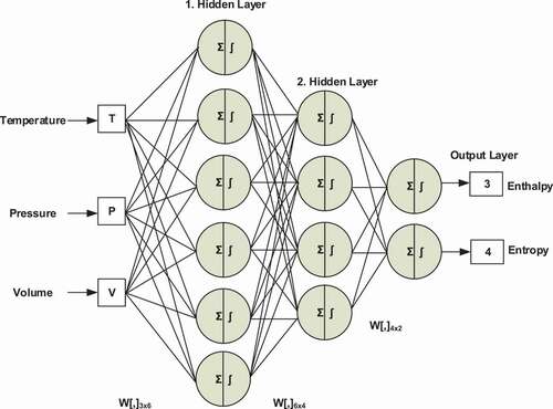
In Figure 4, the proposed AANN model for the SHV region is given. It has three layers as three inputs, two hidden layers, and two outputs. The input parameters of the developed model are temperature, pressure, and volume. Enthalpy and entropy represent the thermodynamic properties of the R404a, which are the output parameters of the proposed model. The outputs are applied to the model separately since the data distribution has completely different characteristics. The third case shows enthalpy and the fourth one shows the entropy parameter of the gas.

Figure 4. The proposed model of the gas under superheated vapor region.

In order to define the best number of neurons for each layer, approximately 50 different network structures have been established. The general feature of these network structures is that the number of neurons will decrease from the first hidden layer to the output. That is the funnel network structure has been adopted. The structure that produces minimum network error was obtained as 6 neurons in the first hidden layer and 4 neurons in the second hidden layer for both the wet vapor and superheated regions.

AANN estimation model is used for enthalpy and entropy data in two different regions (WV and SHV) of the R404a gas for four different experimental data in total. AANN selects a function that provides the lowest error from seven different transfer functions for each model. Thus, the development of a more accurate prediction model is provided as compared to a classical ANN. The optimum combination of transfer functions, that have been developed by AANN, are given in Table 3 for each case. The first and second cases indicate the activation function’s number for the developed AANN’s neurons for the enthalpy and entropy data of R404a under the WV region, respectively. The third and fourth cases indicate the activation function’s number of the developed AANN’s neurons for enthalpy and entropy data of R404a under the SHV region, respectively.

Table 3. The optimum combination of transfer functions for AANN

Cases	The transfer function numbers for first hidden layer	The transfer function numbers for second hidden layer	The transfer function numbers for output layer
1 (WV- Enthalpy)	1-1-2-4-4-1	4-4-1-3	1
2 (WV- Entropy)	6-4-6-1-6-4	1-1-1-4	1
3 (SHV- Enthalpy)	4-4-4-5-6-5	4-4-4-4	1
4 (SHV- Entropy)	4-3-1-2-3-4	6-1-1-1	1

As mentioned above, one of the characteristics of transfer functions of the AANN models is that only a value between zero and one can be produced. The input and output data sets were normalized before the training and testing process to obtain the optimal predictions. Inputs and outputs are normalized (i.e., between the ranges of zero and one) by using the equation below:

(8) $X_{normalized}=\frac{x_i-x_{min}}{x_{max}-x_{min}}$(8)

The performance (accuracy) of the developed model assesses by using multiple metrics such as the root mean squared error (RMSE), the coefficient determination (R²), the mean absolute error (MAE), and the mean absolute percentage error (MAPE). Additionally, the standard deviation of the test value is given in the last row. These statistical criteria may be used to compare the predicted and actual values. During learning, the error is estimated by RMSE.

The root mean square error (RMSE) has been used as a standard statistical metric to measure the model performance. It measures the difference between values predicted by a model and the values actually observed from the environment. The mean absolute error (MAE) is another useful measure widely used in model evaluations. While they have both been used to assess model performance for many years, there is no consensus on the most appropriate metric for model errors (Chai and Draxler 2014; Sahin 2011). The coefficient of determination (R²) represents the variance between predicted and the linear fit data. In other words, it is the percent of closeness to linear fit line. The mean absolute percentage error (MAPE) is one of the most widely used measures of forecast accuracy, due to its advantages of scale-independency and interpretability (Kim and Kim 2016). The formulas of the metric forecast-accuracy metrics are given below.

(9) $RMSE=\sqrt{\frac{1}{n}\sum _{k=1}^n{\left|y_k-{\hat{y}}_k\right|}^2}$(9)

(10) $MAE=\frac{1}{n}\sum _{k=1}^n\left|y_k-{\hat{y}}_k\right|$(10)

(11) $MAPE=\frac{1}{n}\sum _{k=1}^n\frac{\left|y_k-{\hat{y}}_k\right|}{{\hat{y}}_k}\ast 100$(11)

(12) $R^2=1-\left(\frac{\sum _{k=1}^n{\left|y_k-{\hat{y}}_k\right|}^2}{\sum _{k=1}^n{{\hat{y}}_k}^2}\right)$(12)

Where $y_k$ is the real (measured) value, $\widehat{y_k}$ is the predicted value and $n$ is the number of samples.

Experimental Results

In this study, the thermodynamic properties of R404a have two main regions, namely: wet vapor (WV) and superheated vapor (SHV). For both regions, the properties of the gas are as follows. Critical temperature, pressure, density, and volume are 72.07°C, 3731.5 kPa, 484.5 kg/m³, 0.00206 m³/kg, respectively. 1826 experimental data for WV region sets were pre-pared for the training and testing of AANN. The ratio for the training and testing data was selected as 85:15, i.e. 1566 and 260 sets of the experimental data were randomly selected. 2332 experimental data for SHV region sets were pre-pared for the training and testing of AANN. The ratio for training and testing data was selected as 80:20, i.e., 1867 and 465 sets of the experimental data were randomly selected. Additionally, for both regions, the sample patterns are shown in Table 4. The data used has been obtained from the technical information sheet of the DuPont Suva 404a refrigerant gas.

Table 4. Data samples for wet vapor and superheated vapor regions

	Region
Properties	WV			SHV
Temperature (°C)	– 46	65	0	0	–35	100
Vapor Quality	0	1	0.5
Pressure (kPa)	103.5	3194.6	611.1	20	40	70
Specific Volume (m^3/kg)	0.0008	0.0043	0.1715	1.1586	0.501	0.4516
Enthalpy (kJ/kg)	138.1	380.9	284.15	377.3	349.3	468.4
Entropy (kJ/kgK)	0.7537	1.5599	1.3084	1.9289	1.7606	2.1056

As an example, weights and biases obtained from ANN and AANN after training to estimate the Entropy for the saturated region are given in Tables 5 and 6, respectively.

Table 5. Weights and biases of ANN to estimate entropy for saturated vapor region

Inputs to Hidden Layer 1
Nodes	w1	w2	b
1	0,8381	0,9708	−1,2744
2	1,0806	0,5597	−0,4944
3	−1,1463	1,1486	−0,9514
4	−1,3690	1,4580	−1,5069
5	0,7398	−0,6017	−1,0414
6	2,6174	2,4869	0,1608
	Hidden Layer 1 to Hidden Layer 2
Nodes	w1	w2	w3	w4	b
1	0,4641	1,3708	0,0937	1,6346	1,7707
2	0,9779	−0,0255	2,2667	−0,0310	2,9286
3	0,7715	0,9020	0,5005	0,8297	1,1830
4	−1,2663	1,7209	0,3681	0,0427	3,2430
5	0,8038	1,1327	0,0791	0,9435
6	−0,1053	1,3532	−0,1147	2,9183
Hidden Layer to Output (Entropy)
Nodes	w1	b
1	0,4581	0,3695
2	−0,2801
3	0,2126
4	0,0349

Table 6. Weights and biases of AANN to estimate entropy for saturated vapor region

Inputs to Hidden Layer 1
Nodes	w1	w2		b
1	0,9925	0,6106		0,0017
2	−0,2217	1,7342		−0,1268
3	1,2055	1,0952		−0,7525
4	−2,3955	1,6869		−1,8771
5	−0,9506	1,0240		−0,9174
6	1,6921	1,3815		0,2100
Hidden Layer 1 to Hidden Layer 2
Nodes	w1		w2		w3		w4		b
1	0,3668		1,6844		2,9571		−0,3238		2,4294
2	0,6829		−0,0659		1,2723		0,6517		1,9964
3	1,2254		0,8548		0,0591		0,5989		3,3438
4	0,2917		1,6550		0,7400		0,4257		1,7553
5	−0,7648		1,4979		0,6073		2,2368
6	−0,7494		0,5007		1,0572		0,9836
Hidden Layer to Output (Entropy)
Nodes	w1		b
1	−0,2584		0,5979
2	−0,6813
3	0,8404
4	0,4308

The metrics of the accuracy of the developed model are described in the previous section. RMSE is the main stop criteria for the optimization cycle. It is the most important value for the comparison of the developed algorithm. Additionally, standard deviation (SD) values of the errors are given in tables in the last column. It helps to verify the normal distribution of the data.

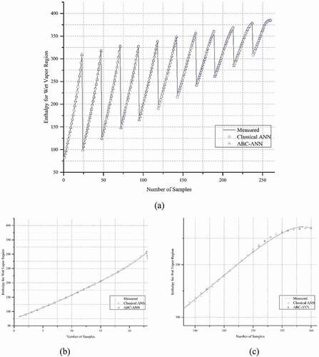
The results of the statistical metrics for enthalpy data at the WV region are given in Table 7. It can be clearly shown that R² results are very close to one. The other metrics are very close to AANN and classical ANN except for MAPE. The difference of the developed model gives a better solution for the MAPE metric. In Figure 5, data regression graphs are given. The comparisons of the measured and predicted data (ANN and AANN) are presented in Figure 6a, which demonstrates the difference between them. As can be seen clearly from the zoomed graphs (Figure 6b,c), the developed hybrid model provides closer results to the measured data line than the classic ANN model.

Table 7. Performance analysis of the prediction algorithms for Enthalpy at WV region

Algorithm	R^2	RMSE	MAE	MAPE	SD
Classical ANN	0,99,997	0,00339	0,00266	0,64,521	0,0021
ABC-ANN	0,99,998	0,00329	0,00265	0,55,950	0,0019

Figure 5. Test data (Enthalpy, WV region) regression graph for ANN and AANN (ABC-ANN).

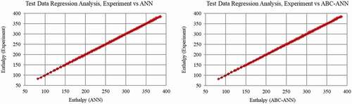
Figure 6. Comparison of measured, ANN and AANN data for Enthalpy, WV region a) all data b) zoom in beginning data c) zoom in last data.

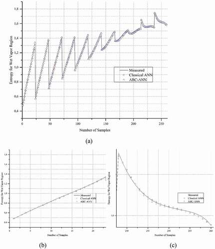
The results of the statistical metrics for entropy data at the WV region are given in Table 8. It can be clearly shown that R² results are very close to one. The other metrics show that visible improvement could be achieved by AANN compared to classical ANN. In Figure 7, data regression graphs are given. The comparisons of the measured and predicted data (classical ANN and AANN) are presented in Figure 8a. As can be seen clearly from the zoomed graphs (Figure 8b,c), the developed hybrid model provides closer results to the measured data line than the classic ANN model.

Table 8. Performance analysis of the prediction algorithms for Entropy at WV region

Algorithm	R^2	RMSE	MAE	MAPE	SD
Classical ANN	0,99,997	0,00340	0,00268	0,60,310	0,0021
ABC-ANN	0,99,998	0,00285	0,00205	0,51,129	0,0017

Figure 7. Test data (Entropy, WV region) regression graph for ANN and AANN (ABC-ANN).

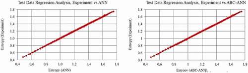
Figure 8. Comparison of measured, ANN and AANN data for Entropy, WV region a) all data b) zoom in beginning data c) zoom in last data.

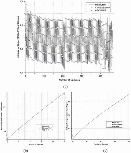
The results of the statistical metrics for entropy and enthalpy data at the SHV region are given in Tables 9 and 10, respectively. It is shown that R² results are very close to one. The other error metrics (RMSE, MAE, MAPE, and SD) are under the acceptable threshold. The developed adaptive model (AANN) achieves a serious improvement as compared to the classical ANN. In Figs. 9 and 11, data regression plots are given for enthalpy and entropy, respectively. Fig. 10a-c and Fig. 12a-c were obtained to compare and evaluate the performance of the developed model.

Table 9. Performance analysis of the prediction algorithms for Enthalpy at SHV region

Algorithm	R^2	RMSE	MAE	MAPE	SD
Classical ANN	0,99,998	0,00205	0,00161	1,78,711	0,0013
ABC-ANN	0,99,999	0,00117	0,00080	1,26,715	0,0009

Table 10. Performance analysis of the prediction algorithms for Entropy at SHV region

Algorithm	R^2	RMSE	MAE	MAPE	SD
Classical ANN	0,99,989	0,00522	0,00418	1,09859	0,0031
ABC-ANN	0,99,994	0,00389	0,00321	0,96,811	0,0022

Figure 9. Test data (Enthalpy, SHV region) regression graph for ANN and AANN (ABC-ANN).

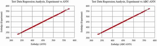
Figure 10. Comparison of measured, ANN and AANN data for Enthalpy, SHV region a) all data b) zoom in beginning data c) zoom in last data.

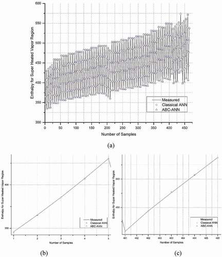
Figure 11. Test data (Entropy, SHV region) regression graph for ANN and AANN (ABC-ANN).

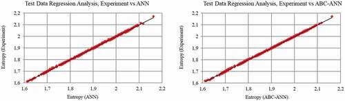
Figure 12. Comparison of measured, ANN and AANN data for Entropy, SHV region a) all data b) zoom in beginning data c) zoom in last data.

In Table 11, some samples consisting of real values and calculated values with ANN and AANN have been given. Moreover, error values between real and calculated values obtained from both methods have been presented. It is clearly seen that AANN provides a decreased error of the model. The last column represents the improvement of percentage error reduction (IPER). The calculation equation of the improvement as a percentage is given below.

(13) $E_{reduction}=\frac{E_{AANN}-E_{ANN}}{E_{ANN}}\times 100$(13)

Table 11. Comparison of real and calculated h and s values

	Real	ANN	AANN	Error ANN	Error AANN	IPER
Case-1 Enthalpy (h) WV (kJ/kg)	82,1000	82,5931	82,2524	0,4931	0,1524	69%
	137,4900	138,9136	137,9281	1,4236	0,4381	69%
	200,0600	200,1748	199,9467	0,1148	0,1133	1%
	328,8000	329,0916	328,7641	0,2916	0,0359	88%
Case-2 Entropy (s) WV (kJ/kgK)	0,7489	0,7450	0,7485	0,0039	0,0004	90%
	0,4781	0,4805	0,4787	0,0024	0,0006	75%
	1,1683	1,1613	1,1683	0,0070	0,0000	100%
	1,6440	1,6397	1,6454	0,0043	0,0014	67%
Case-3 Enthalpy (h) SHV (kJ/kg)	550,8000	549,4844	549,8028	1,3156	0,9972	24%
	348,8000	348,4706	348,7368	0,3294	0,0632	81%
	411,1000	411,5447	411,4506	0,4447	0,3506	21%
	476,2000	476,4546	476,1729	0,2546	0,0271	89%
Case-4 Entropy (s) SHV (kJ/kgK)	1,8642	1,8633	1,8640	0,0009	0,0002	78%
	2,0430	2,0461	2,0440	0,0031	0,0010	68%
	1,6422	1,6402	1,6412	0,0020	0,0010	50%
	1,9454	1,9486	1,9442	0,0032	0,0012	63%

The improvements of the percentage error reduction (IPER) were calculated for all the test data and represented in Table 12. According to results, the errors of the model has been reduced thanks to the presented/proposed AANN. Thus, the thermodynamics properties of R404a were estimated more accurately as compared to classical ANN. In Case-4, the improvement of percentage is higher than other cases. This is most probably because the randomly selected test data is predicted by the ANN with greater error.

Table 12. Improvements of percentage error (IPER)

	ANN	AANN	IPER
Case – 1	0,3549	0,3281	7,55
Case – 2	0,3084	0,2485	19,41
Case – 3	0,1062	0,0328	8,34
Case – 4	0,1313	0,0103	76,68

Conclusion

In this study, an adaptive ANN model is proposed to model the thermodynamic properties of the environmentally friendly refrigerant gas (R404a) for both the saturated liquid–vapor region (wet vapor) and superheated vapor region.

One of the biggest disadvantages of ANN, which has a strong modeling ability between its complex network structure and inputs as well as outputs, is the necessity of choosing the correct parameters. The classical ANN uses a predefined activation function to calculate the neurons’ output. In this sense, the correct selection of the activation functions leads to both the modeling accuracy of the ANN and the prolongation of the time to obtain the parameters in the modeling. The developed adaptive model updates these functions dynamically per each layer. In this developed model, in order to define the optimal combination of the activation function of neurons, the ABC algorithm has been used as a heuristic search unit. The developed model has been applied to test data and the results obtained have been compared with classical ANN results. The main metric of the performance of the developed model is R² and it is closer to one. The other metrics show that the AANN gives a better performance than the classical ANN. The improvements of percentage error reduction (IPER) are improved by AANN. Thus, empirical equations of the thermodynamic properties of the R404a calculate more accurately. In further studies, if the thermodynamic properties are unknown, modeling can be performed with less experimentation by using a heuristic-based algorithm to develop properties (instead of the Mollier Chart). Deep learning-based neural networks or derivatives can be studied in the general modeling of gases.

Disclosure statement

No potential conflict of interest was reported by the author(s).

References

- Ahmed, R., S. Mahadzir, N. E. M. Rozali, K. Biswas, F. Matovu, and K. Ahmed. 2021. Artificial intelligence techniques in refrigeration system modelling and optimization: A multi-disciplinary review. Sustainable Energy Technologies and Assessments 47:101488. doi:https://doi.org/10.1016/j.seta.2021.101488.
- Atalay, H., and M. T. Coban. 2015. Modeling of thermodynamic properties for pure refrigerants and refrigerant mixtures by using the helmholtz equation of state and cubic spline curve fitting method. Universal Journal of Mechanical Engineering 3 (6):229–51. doi:https://doi.org/10.13189/ujme.2015.030604.
- Awan, S. M., M. Aslam, Z. A. Khan, and H. Saeed. 2014. An efficient model based on artificial bee colony optimization algorithm with neural networks for electric load forecasting. Neural Computing & Applications 25 (7–8):1967–78. doi:https://doi.org/10.1007/s00521-014-1685-y.
- Chai, T., and R. R. Draxler. 2014. Root mean square error (RMSE) or mean absolute error (MAE)? - Arguments against avoiding RMSE in the literature. Geoscientific Model Development 7 (3):1247–50. doi:https://doi.org/10.5194/gmd-7-1247-2014.
- Coquelet, C., J. El Abbadi, and C. Houriez. 2016. Prediction of thermodynamic properties of refrigerant fluids with a new three-parameter cubic equation of state. International Journal of Refrigeration-Revue Internationale Du Froid 69:418–36. doi:https://doi.org/10.1016/j.ijrefrig.2016.05.017.
- Doubek, M. 2018. “Thermophysical properties of refrigerants: Experiment and simulations.” PhD, Faculty of Mechanical Engineering, Czech Technical University
- Dursun, M., and S. Ozden. 2017. Optimization of soil moisture sensor placement for a PV-powered drip irrigation system using a genetic algorithm and artificial neural network. Electrical Engineering 99 (1):407–19. doi:https://doi.org/10.1007/s00202-016-0436-8.
- Efkolidis, N., A. Markopoulos, N. Karkalos, C. G. Hernández, J. L. H. Talón, and P. Kyratsis. 2019. Optimizing models for sustainable drilling operations using genetic algorithm for the optimum ANN. Applied Artificial Intelligence 33 (10):881–901. doi:https://doi.org/10.1080/08839514.2019.1646014.
- Karaboga, D. 2005. An idea based on honey bee swarm for numerical optimization. Turkey: Erciyes University, Engineering Faculty.
- Karaboga, D., and B. Akay. 2009. A comparative study of Artificial Bee Colony algorithm. Applied Mathematics and Computation 214 (1):108–32. doi:https://doi.org/10.1016/j.amc.2009.03.090.
- Karaboga, D., and B. Basturk. 2007. A powerful and efficient algorithm for numerical function optimization: Artificial bee colony (ABC) algorithm. Journal of Global Optimization 39 (3):459–71. doi:https://doi.org/10.1007/s10898-007-9149-x.
- Karaboga, D., and B. Basturk. 2008. On the performance of artificial bee colony (ABC) algorithm. Applied Soft Computing 8 (1):687–97. doi:https://doi.org/10.1016/j.asoc.2007.05.007.
- Karaboga, D., and C. Ozturk. 2009. Neural networks training by Artificial Bee Colony algorithm on pattern classification. Neural Network World 19 (3):279–92.
- Karaboga, D., and C. Ozturk. 2011. A novel clustering approach: Artificial Bee Colony (ABC) algorithm. Applied Soft Computing 11 (1):652–57. doi:https://doi.org/10.1016/j.asoc.2009.12.025.
- Kim, S., and H. Kim. 2016. A new metric of absolute percentage error for intermittent demand forecasts. International Journal of Forecasting 32 (3):669–79. doi:https://doi.org/10.1016/j.ijforecast.2015.12.003.
- Kizilkan, O. 2011. Thermodynamic analysis of variable speed refrigeration system using artificial neural networks. Expert Systems with Applications 38 (9):11686–92. doi:https://doi.org/10.1016/j.eswa.2011.03.052.
- Mohanraj, M., S. Jayaraj, and C. Muraleedharan. 2012. Applications of artificial neural networks for refrigeration, air-conditioning and heat pump systems—A review. Renewable and Sustainable Energy Reviews 16 (2):1340–58. doi:https://doi.org/10.1016/j.rser.2011.10.015.
- Mohebbi, A., M. Taheri, and A. Soltani. 2008. A neural network for predicting saturated liquid density using genetic algorithm for pure and mixed refrigerants. International Journal of Refrigeration 31 (8):1317–27. doi:https://doi.org/10.1016/j.ijrefrig.2008.04.008.
- Mora, R., . J. E., C. Pérez T, F. F. González N, and J. D. Ocampo D. 2014. Thermodynamic properties of refrigerants using artificial neural networks. International Journal of Refrigeration 46:9–16. doi:https://doi.org/10.1016/j.ijrefrig.2014.07.007.
- Neto, M. A. M., and J. R. Barbosa. 2010. Modeling of state and thermodynamic cycle properties of HFO-1234yf using a cubic equation of state. Journal of the Brazilian Society of Mechanical Sciences and Engineering 32 (5):461–67. doi:https://doi.org/10.1590/S1678-58782010000500005.
- Ozturk, C., and D. Karaboga. 2011. Hybrid Artificial Bee Colony algorithm for neural network training. IEEE Congress on Evolutionary Computation 84–88. New Orleans, LA, USA https://doi.org/https://doi.org/10.1109/CEC.2011.5949602
- Sahin, A. S. 2011. Performance analysis of single-stage refrigeration system with internal heat exchanger using neural network and neuro-fuzzy. Renewable Energy 36 (10):2747–52. doi:https://doi.org/10.1016/j.renene.2011.03.009.
- Sahin, A. S., T. Kovacı, and E. Dikmen. 2021. A GEP-based model approach for estimating thermodynamic properties of R513A refrigerant. El-Cezerî Journal of Science and Engineering 8 (1):376–88. doi:https://doi.org/10.31202/ecjse.814527.
- Şencan, A., İ. İ. Köse, and R. Selbaş. 2011. Prediction of thermophysical properties of mixed refrigerants using artificial neural network. Energy Conversion and Management 52 (2):958–74. doi:https://doi.org/10.1016/j.enconman.2010.08.024.
- Shah, H., R. Ghazali, N. M. Nawi, and M. M. Deris. 2012. Global hybrid ant bee colony algorithm for training artificial neural networks. Computational Science and Its Applications 7333:87–100.
- Shunmugapriya, P., and S. Kanmani. 2017. A hybrid algorithm using ant and bee colony optimization for feature selection and classification (AC-ABC Hybrid). Swarm and Evolutionary Computation 36 (Supplement C):27–36. doi:https://doi.org/10.1016/j.swevo.2017.04.002.
- Sonmez, Y. 2013. Estimation of fuel cost curve parameters for thermal power plants using the ABC algorithm. Turkish Journal of Electrical Engineering and Computer Sciences 21:1827–41. doi:https://doi.org/10.3906/elk-1203-10.
- Sonmez, Y., U. Guvenc, H. T. Kahraman, and C. Yilmaz. 2015. A comperative study on novel machine learning algorithms for estimation of energy performance of residential buildings. 3rd International Istanbul Smart Grid Congress and Fair. Istanbul, Turkey https://doi.org/https://doi.org/10.1109/SGCF.2015.7354915
- Sözen, A., E. Arcaklioğlu, and T. Menlik. 2010. Derivation of empirical equations for thermodynamic properties of a ozone safe refrigerant (R404a) using artificial neural network. Expert Systems with Applications 37 (2):1158–68. doi:https://doi.org/10.1016/j.eswa.2009.06.016.
- Tsai, H. C. 2014. Integrating artificial bee colony and bees algorithm for solving numerical function optimization. Neural Computing & Applications 25 (3–4):635–51. doi:https://doi.org/10.1007/s00521-013-1528-2.
- Zyczkowski, P., M. Borowski, R. Luczak, Z. Kuczera, and B. Ptaszynski. 2020. Functional equations for calculating the properties of low-GWP R1234ze(E) refrigerant. Energies 13 (12):12. doi:https://doi.org/10.3390/en13123052.