A DBN-DEVS Extension for Modeling and Simulate Uncertain Systems

ABSTRACT

In this paper, our goal is to propose a new extension to the Discrete Event System (DEVS) formalism, which is based on Dynamic Bayesian Network (DBN), and this extension will be called DBN-DEVS, which allows to modeling and simulate the uncertain behavior of complex systems. To gain their modeling power, we will integrate the Dynamic Bayesian Network which will allow DEVS to be useful for a wide range of applications domain. To test and validate our extension, we took the field of intrusion detection to model the uncertain behavior of IDS during prediction intrusion detection.

Introduction

To propose incorporation of uncertainty into DEVS concepts, most of the works has concerned the introduction of fuzzy notions (Kwon et al. 1996). Fuzzy-DEVS modeling and simulation can be practical in the study of different kinds of systems such as the case of the modeling of systems, for which we have few observations of how and where the actor being actions as a sensor or expert.

Table 1. Observed actions in DARPA 2000

DDoS steps	Actions
Phase1	A1: icmp_ping, A6: icmp_reply A11: icmp_port_unreachable
Phase2	A2: rpc_sadmind_request A3: sadmind_ping
Phase3	A4: sadmind_root_query A5: sadmind_bof, A10: rsh_root
Phase4	A7: telnet_info A8: telnet_login_incorrect A9: telnet_bad_login
Phase5	A12: launch DDoS

Table 2. Preprocessed observation data for a DDoS attack

Action1	Action2	… …	ActionN	Phase =
1	1	… …	0	Ph1
0	0	… …	1	Ph5
… …	… …	… …	… …	… …

Table 3. Test result

Actions	P(DDoS/Action,Phase)
A1	19%
A1 A6	28%
Phase1 A2	70%
Phase1 A2 A3	100%
Phase2 A4 A5	100%
Phase3 A7	100%
Phase3 A7 A8	100%
Phase3 A7 A8 A9	100%

The study of uncertain systems thus requires the integration of several techniques within a model. To take into account uncertain transition, we propose to define an approach allowing the addition of a technique based on Dynamic Bayesian Network DBN, in the environment of DEVS.

In the DEVS formalism, Zeigler (1976) introduced the concept of external transition function δ_ext that represents the response of the system to the input events. The system is in a state S_t at a time t. An external event occurs, then the function δ_ext indicates what is the new state S_t+1 of the system according to S_t.1. In this work, our goal is to define this function in case of uncertain transition to predict the new state St+1 of system that according to both external events and actual state St (sequential system).

The first part introduces the basic concepts of our work: DEVS and DBN theory. The second part proposes a general vision of our approach of modeling and presents our caption methodology of DBN modeling. The third part, an example allows illustrating the feasibility of the approach inside the DEVS environment. Finally, a conclusion recapitulates the essential points of our work and provides prospects for the work that remains to do.

Related Works

A several extensions of DEVS have been presented for the modeling and simulation of complex dynamic systems, which are based on computational method. Among those approaches, we can cite:

NEURO-DEVS

This extension proposed by (Filippi, Bisgambiglia, and Delhom 2002) is an hybrid methodology to describe complex systems. In this work, authors have proposed an approach to extend Object Oriented Modeling and Simulation environment (JDEVS) with neural network objects.

The Neuro-DEVS environment proposes an alternative with three main applications of the environment:

1. Concurrent simulation can be used to avoid an unexpected behavior of a neural network by comparing the neural network output with the output of a simple model to validate the result.

2. Adaptive models can be used to modify the neural network runtime according to an error (difference between the model’s forecast and the real-world data collected afterward).

3. Artificial Neural Network as a sub-component can be used if Neural Networks provides better results for only a piece of the whole system.

Fuzz-iDEVS

In this work, authors (Bisgambiglia, Innocenti, and Bisgambiglia 2018) have proposed Fuzz-iDEVS extension that is based on definitions of the Fuzzy Set Theory to represent and use imprecise information in the DEVS formalism. The goal of authors was to present a generalization to DEVS for be able to adapt with imprecision in all of its elements (events, transition functions, state). Authors propose to extend the DEVS formalism toward the Fuzzy Set Theory (FST). This approach differs compared to (Kwon et al. 1996) considering all model parameters, especially the values (X, Y, S, ta) and not only the state transitions functions. This method wish for model imprecision and not uncertainty.

NB-DEVS

In another work, Mostefaoui and Dahmani (2019) present a new approach (NB-DEVS) of modeling for discrete events systems that allow specification of uncertain parameters systems. This work based on the integration of naïve Bayesian Network in the DEVS formalism offers the possibility to deal with the uncertainties in transitions between states.

Background

The DEVS Formalism

The DEVS formalism is a modeling approach based on the general theory of systems. More precisely, it is a modular and hierarchical formalism for modeling, centered on the notion of state. A system is represented, for its structural form, by two types of models.

Modeling involves interconnecting these different types of models to form a new model describing the behavior of the studied system, it is the functional aspect.

Atomic models are the basic components of formalism; they describe the behavior of the system. Their operation is similar to that of state machines.

A DEVS system consists of atomic and coupled models. An atomic model presents behavior, while a coupled model describes structure. A coupled model is a net of nested models, which can be either atomic or coupled.

An atomic model is presented as a septet$M=\left(X,Y,S,ta,{\delta }_{ext},{\delta }_{int},\lambda \right)$ where:

• X is the set of input events. If there are more than one input ports, the input events are represented as doubles$\left(p,v\right)$, where p is the input port and v is the received value.

• The same principle applies for the set of output events Y.

• S is the set of states. The model always finds itself in just one state.

• Time advance function$\mathrm{t}\mathrm{a}:S\to {\mathbb{R}}^{\ast }$, where ${ }^{\ast }={\cup }^{\left\{\mathrm{\infty }\right\}}$, defines duration of each state.

• The external transition function ${\delta }_{ext}:\mathrm{Q}\mathrm{x}\mathrm{X}\to \mathrm{S}$, where $\mathrm{Q}=\left\{\left(\mathrm{s},\mathrm{e}\right)\left|\mathrm{s}\in \mathrm{S},\mathrm{e}\in \left[0,\mathrm{t}\mathrm{a}\left(\mathrm{s}\right)\right]\right.\right\}$, defines how the model responds to an incoming event considering the time e elapsed from the last event, or in other words, which state will become the new current state.

• The internal transition function ${\delta }_{int}:\mathrm{S}\to \mathrm{S}$ defines which state becomes the new current state after the time elapsed exceeds the current state’s lifespan.

• The output function $\lambda :S\to Y$ defines how a state of the system generates an output event when the elapsed time reaches to the lifetime of the state.

DBNs: Representation

A DBN (Dean and Kanazawa 1989) is a technique to extend Bayes networks (BN) to represent probability distributions about collections of random variables, X₁, X₂ … . We only consider discrete time stochastic processes, so we increase the index t by one every time a latest observation arrives. The observation could represent that something has changed, making this a model of a discrete-event system. The term dynamic means a modeling of dynamic system, not that the structure changes over time.

A DBN comprises a BN which defines the prior$\mathrm{P}\left({\mathrm{X}}_1\right)$, and a two-slice temporal BN (2TBN) which defines $\mathrm{P}\left({\mathrm{X}}_{\mathrm{t}}\left|{\mathrm{X}}_{\mathrm{t}-1}\right.\right)$ by a DAG (directed acyclic graph) as follows:

(1) $P\left(X_t\left|X_{t-1}\right.\right)=\prod _{i=1}^{N}P\left(X_t^i\left|Pa\left(X_t^i\right)\right.\right)$(1)

where ${\mathrm{X}}_{\mathrm{t}}^{\mathrm{i}}$ is the i’ th node at time t and $\mathrm{P}\mathrm{a}\left({\mathrm{X}}_{\mathrm{t}}^{\mathrm{i}}\right)$ are the parents of ${\mathrm{X}}_{\mathrm{t}}^{\mathrm{i}}$ in the graph. The nodes in the initial slice of a 2TBN do not have any parameters associated with them, but each node in the next slice of the 2TBN (two-slice temporal Bayes net) has an related conditional probability distribution (CPD), which defines $P\left(X_t^i\left|Pa\left(X_t^i\right)\right.\right)$ for $t>1$.

The arcs between slices are from left to right, presenting the causal flow of time. If there is an arc starting from $X_{t-1}^i$ to $X_t^i$, this node will be called persistent.

The semantics of a dynamic Bayesian network can be defined by unrolling the 2TBN until T time-slices. The JD (joint distribution) is then given by:

(2) $P\left(X_{1:T}\right)=\prod _{t=1}^T\prod _{i=1}^{N}P\left(X_t^i\left|Pa\left(X_t^i\right)\right.\right)$(2)

Proposed Approach

The section introduces the concepts that have been defined to integrate DBN into DEVS models. We try to present our approach that allows defining the process for the mapping from a given input to an output and state transition using DBN.

Our work begins from the limitations presented in the work of Mostefaoui and Dahmani (2019). In those work, authors presented an idea by coupling DEVS and Naïve Bayes Network, but their proposed model presents a major problem when they placed the same node representing a states (S_i, S_i+), in different layers of their Naive Bayesian model (

Figure 1. DEVS atomic model.

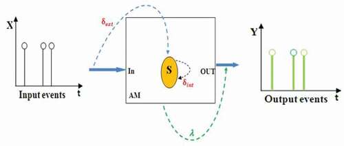
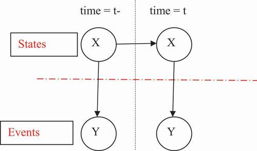
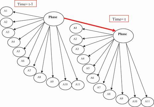
Figure 2. Example of 2DBN.

Figure 3).

Figure 3. Example of 2DBN (Mostefaoui and Dahmani 2019).

This conception prevents us to modeling a dynamic system when:

1. System states aren’t temporal variables, in fact the variables S_i, S_i+ become same, and in this case, we have cyclic causality relation, so we are talking about a non-DAG (Directed Acyclic Graph) model.

2. At the beginning, prevision of the next state S₁ requires knowledge of P(S₀) like a prior probability (observation, evidence), which is impossible when initial state is unknown.

To resolve this problem, we will integrate DBN into DEVS that allows prediction of initial state of system by representing BN in different level of time. To succeed in this integration, the following supplies have to be fulfilled:

Specify a DBN Model Structure that Describes a System

When the states of our dynamic model (system) do not need to be directly observable, they may influence some other variables (extern events) that we can directly measure. Also, the behavior (states) of our system isn’t a unique (simple state), it may be considered as a complex structure of states. Each state in our dynamic model at one slice (time instance) may depend on one or more states at the previous slice (t-1) and (or) on some variables (extern events) in the same time instance (slice t).

Now, we can specify our DBN model saying that it consists of probability distribution function on the sequence of T variables (states) $X=\left\{x_1,\dots ,x_T\right\}$ and the sequence of T observable variables (extern events) $Y=\left\{y_1,\dots ,y_T\right\}$. This can be expressed by:

(3) $P\left(X,Y\right)=\prod _{t=2}^{T}P\left(x_t\left|x_{t-1}\right.\right)\prod _{t=1}^{T}P\left(y_t\left|x_t\right.\right)P\left(x_1\right)$(3)

Learning Parameters of DBN

The structure of the network is already defined; we have to calculate the distribution of probabilities. The observation data (Corpus) [Dataset , 2000] allow us to estimate the distributions of conditional probabilities that can be made by a simple frequency calculation. Once the observations (states) are obtained and formatted (corpus), we can calculate the probability distribution (parameters) for each variable. In this step, we will define three sets of parameters:

1. Prior State Distribution $P\left(X\right)$, that Brings Initial Probability Distribution in the Start of Process.

The probability of observing the state of the system $P\left(X=x\right)$, can be calculated as follows:

(4) $P\left(X=x\right)=\frac{NB\left(X=x\right)}{N}$(4)

Where

• x is the value of a state.

• NB (X = x): Number of lines where state = x.

• N: the size of corpus (total number of lines).

2. State transition probability distribution function $P\left(x_t=\mathrm{a}\left|x_{t-1}=\mathrm{b}\right.\right)$ that specifies time dependencies between the states.

(5) $P\left(x_t=\mathrm{a}\left|x_{t-1}\right.=\mathrm{b}\right)=\frac{NB\left(x_t=aand{x}_{t-1}=b\right)}{NB\left(x_{t-1}=b\right)}$(5)

where

• $a,b\in \left\{valuesofstate\right\}$.

• $NB\left(x_t=aand{x}_{t-1}=b\right)$ Number of lines where state = a in time t and state = b in time t-1.

• $NB\left(x_{t-1}=b\right)$: Number of lines where state = b in time t-1.

3. Observation probability distribution function$P\left(y_t\left|x_t\right.\right)$ that specifies the conditional probability distribution of external events in the context of the state at time slice t. This probability can be calculated as follows:

(6) $P\left(y_t=e\left|x_t\right.=s\right)=\frac{NB\left(y_t=eand{x}_t=s\right)}{NB\left(x_t=s\right)}$(6)

where

• $s\in \left\{valuesofstate\right\}ande\in \left\{valuesofexternalevents\right\}$

• $NB\left(y_t=e\mathrm{a}\mathrm{n}\mathrm{d}{x}_t=s\right)$ Number of lines where external event = e in slice time t and state = s in the same slice time.

• $NB\left(x_t=s\right)$: Number of lines where state = s.

Inference for Prediction of New State

At the stage, our goal is to define external transition function (DEVS) by estimating the probability distribution function for predicting next state $X_{t+1}$ given observations (extern events) $Y_{t+1}$ and actual state $X_t$ of system.

Formally, this objective will be realized by estimation of $P\left(X_{t+1}\left|X_{t,}\right.Y_{t+1}\right)$

We have probability distribution function

$P\left(X_{t+1},X_t,Y_{t+1}\right)=P\left(X_t\right)P\left(X_{t+1}\left|X_t\right.\right)P\left(Y_{t+1}\left|X_t\right.\right)$

and

$P\left(X_{t+1},X_t,Y_{t+1}\right)=P\left(X_t\right)P\left(Y_{t+1}\right)P\left(X_{t+1}\left|X_{t,}\right.Y_{t+1}\right)$

Then

$P\left(X_{t+1}\left|X_t=x\right.,Y_{t+1}=y\right)=\frac{P\left(X_{t+1}\left|X_t\right.\right)P\left(Y_{t+1}=y\left|X_t=x\right.\right)}{P\left(Y_{t+1}=y\right)}$

(7) $=\frac{1}{\alpha }P\left(X_{t+1}\left|X_t\right.\right)P\left(Y_{t+1}\left|X_t=x\right.\right)$(7)

Note that α is a constant that can be obtained by normalization.

Now, we can predict the next state of our system by calculating

(8) $X_{t+1}=\underset{s\in S}{argmax}P\left(X_{t+1}=s\left|X_t=x\right.,Y_{t+1}=y\right)$(8)

where $s\in \left\{valuesofstate\right\}$

Simulation algorithm

Variables:

DEVS = < X, Y, S, δext_inc, δint, λ, ta >

t_l // last event time

t_n // next event time

x // current external event

y // current output of the model

s_c // current state

s_n // next state

Receiving i-message (i, t) at time t:

t_l ← t – e

t_n ← t_l +ta(s)

Receiving *-message (*,t) at time t:

if (t ! = tn) then Error: bad synchronization

y ← λ (s)

s ← δ_int(s)

t_l ← t

t_n ← t_l +t_a(s)

Receiving x-message (x,t) at time t with input x:

t_l ← 0

t_n ← 0

if !(t_l ≤ t≤ t_n) then

Error: bad synchronization

e ← t – t_l

if (t_l = = 0) then // Prediction of initial state which is unknown

${\mathrm{s}}_{\mathrm{n}}\leftarrow {\delta }_{ext}\left(\left({\mathrm{s}}_{\mathrm{l}},\mathrm{e}\right),\mathrm{x}\right)=\underset{s\in S}{argmax}P(s|x)$

else

${\mathrm{s}}_{\mathrm{n}}\leftarrow {\delta }_{ext}\left(\left({\mathrm{s}}_{\mathrm{l}},\mathrm{e}\right),\left(\mathrm{x}\right)\right)=\underset{s\in S}{argmax}P(s|s_c,x)$

Endif

t_l ← t

t_n ← t_l +ta(s_n)

Example and Modeling

Now, we will model the behavior of an Intrusion Detection System (IDS) that monitors a network or systems for malicious activity or policy violations, by taking advantage of available historical data, and provides efficient model for analyzing, detecting, and predicting most plausible attack scenario.

However, intruders can use complex attacks to achieve their goals. Often, they perform a series of actions (elementary attacks) in a well-defined sequence, called “scenario” or “plan of attack.” Most of these actions are reported by IDSs, but the logical relationships between these actions (sequence of actions) are not detected by standard tools. Thus, system administrators are often submerged by a large volume of alerts to correlate manually. To this end, the goal of the correlation is to research relationships between alerts.

Few studies have applied Bayesian Networks (RBs) to alert correlation (Benferhat, Kenaza, and Mokhtari 2008; Geib and Goldman 2001; Qin and Lee 2004). In this paper, we present a new approach to alert correlation based on DBN for detecting coordinated attacks. Our approach is effective for predicting attack scenarios and does not involve a great deal of expert knowledge. The alert correlation process will be considered in this article as a classification problem. Given a set of recently observed actions and a set of intrusion objectives, our goal is to determine the most plausible intrusion objectives.

Our approach will be illustrated on first scenario of Defense Advanced Research Projects Agency (DARPA) 2000 Data (datasets, 2000) that includes Distributed Denial of Service (DDoS) driven by a novice attacker. The goal of this attack is that a relatively novice attacker tries to demonstrate his performance using a “script” attack to compromise multiple hosts on the Internet, install the necessary components to conduct a DDoS, and then launch a DDoS against a government site. In this attack, the opponent exploits a flaw in the Sadmind tool (remote administration tool) to gain root access in three Solaris hosts on the Eyrie Air Force Base (AFB) site. The phases of the attack scenario are:

1. Phase1: Scan AFB site from a remote site.

2. Phase2: Find IP addresses of Solaris hosts running Sadmind.

3. Phase3: Compromise of hosts via the vulnerability of Sadmind.

4. Phase4: Installation of the mstream DDoS Trojan on the three hosts of the AFB site.

5. Phase5: Launch of DDoS.

In phase 1, the intruder performs an IPsweep of several subnets on the AFB site. It sends ICMP-echo requests in this scan and listens for ICMP-echo reply to determine which hosts are in place. In phase 2, the discovered hosts are queried to determine which ones execute Sadmind. In phase 2, the discovered hosts are queried to determine which ones execute Sadmind. In Phase 3, the intruder attempts to compromise the hosts running Sadmind. The attacker tries to exploit Sadmind several times in each host, each time with different parameters. At the end of this phase, the intruder obtains root access on three hosts. In phase 4, the attacker performs a telnet connection on the compromised hosts and installs the necessary components for the DDoS (mstrem server and mstream client). In the last phase, the intruder launches the DDoS against the victim.

Construction of the DBN

To build the DBN, we will perform some preprocessing on the observation data. The data contains a set of alerts that report the actions performed and also information on each intrusion phase (whether or not it has been reached). We will first group the DDoS observed phases in a single class called “Phase-Intrusion” and we assign to each phase a number between 0 and 5. The class will contain the values: Domain (class) = {0, Ph1, Ph2, Ph3, Ph4, Ph5} (0 means no phase is reached).

Thus, we will obtain the observations in the form of vectors marked by one or more actions from 0 to N. These actions represent all the variables of the DBN. We have also observed a successful DDoS attack against some hosts, so this intrusion objective will represent the class of DBN.

Figure 4 shows the DBN of the first DARPA 2000 scenario. The network structure is already defined, and it remains for us to calculate the distribution probability.

Figure 4. DBN model.

Figure 5. DDoS DBN model.

As it was defined in the precedent section, we can calculate:

1. Prior state distribution $P\left(Phase\right)$:

(9) $P\left(Pahse=x\right)=\frac{NB\left(Phase=x\right)}{N}$(9)

Where:

• $x\in \left\{0,Ph1,Ph2,Ph3,Ph4,Ph5\right\}$.

• NB (Phase = x): Number of lines where Phase = x.

• N: the size of corpus (total number of lines).

1. Observation probability distribution function. $\mathrm{P}\left({\mathrm{A}}_{\mathrm{n}}^{\mathrm{t}}\left|\mathrm{P}\mathrm{h}\mathrm{a}\mathrm{s}{\mathrm{e}}_{\mathrm{t}}\right.\right)$

(10) $P\left({\mathrm{A}}_{\mathrm{n}}^{\mathrm{t}}=\mathrm{a}\left|\mathrm{P}\mathrm{h}\mathrm{a}\mathrm{s}{\mathrm{e}}_{\mathrm{t}}=\mathrm{s}\right.\right)=\frac{\mathrm{N}\mathrm{B}\left({\mathrm{A}}_{\mathrm{n}}^{\mathrm{t}}=\mathrm{a}\mathrm{a}\mathrm{n}\mathrm{d}\mathrm{P}\mathrm{h}\mathrm{a}\mathrm{s}{\mathrm{e}}_{\mathrm{t}}=\mathrm{s}\right)}{\mathrm{N}\mathrm{B}\left(\mathrm{P}\mathrm{h}\mathrm{a}\mathrm{s}{\mathrm{e}}_{\mathrm{t}}=\mathrm{s}\right)}$(10)

where:

• $s\in \left\{0,Ph1,Ph2,Ph3,Ph4,Ph5\right\}$ and $a\in \{0,1\}$.

• $\mathrm{N}\mathrm{B}\left({\mathrm{A}}_{\mathrm{n}}^{\mathrm{t}}=\mathrm{a}\mathrm{a}\mathrm{n}\mathrm{d}\mathrm{P}\mathrm{h}\mathrm{a}\mathrm{s}{\mathrm{e}}_{\mathrm{t}}=\mathrm{s}\right)$ Number of lines where Action = a in slice time t and $\mathrm{P}\mathrm{h}\mathrm{a}\mathrm{s}{\mathrm{e}}_{\mathrm{t}}=\mathrm{s}$ in the same slice time.

• $NB\left(\mathrm{P}\mathrm{h}\mathrm{a}\mathrm{s}{\mathrm{e}}_{\mathrm{t}}=\mathrm{s}\right)$: Number of lines where $\mathrm{P}\mathrm{h}\mathrm{a}\mathrm{s}{\mathrm{e}}_{\mathrm{t}}=\mathrm{s}$ at time t.

1. Phase transition $\mathrm{P}\left(\mathrm{P}\mathrm{h}\mathrm{a}\mathrm{s}{\mathrm{e}}_{\mathrm{t}+1}\left|\mathrm{P}\mathrm{h}\mathrm{a}\mathrm{s}{\mathrm{e}}_{\mathrm{t}}\right.\right)$.

$P\left(\mathrm{P}\mathrm{h}\mathrm{a}\mathrm{s}{\mathrm{e}}_{\mathrm{t}+1}=\mathrm{a}\left|\mathrm{P}\mathrm{h}\mathrm{a}\mathrm{s}{\mathrm{e}}_{\mathrm{t}}=\mathrm{b}\right.\right)=\frac{\mathrm{N}\mathrm{B}\left(\mathrm{P}\mathrm{h}\mathrm{a}\mathrm{s}{\mathrm{e}}_{\mathrm{t}+1}=\mathrm{a}\mathrm{a}\mathrm{n}\mathrm{d}\mathrm{P}\mathrm{h}\mathrm{a}\mathrm{s}{\mathrm{e}}_{\mathrm{t}}=\mathrm{b}\right)}{\mathrm{N}\mathrm{B}\left(\mathrm{P}\mathrm{h}\mathrm{a}\mathrm{s}{\mathrm{e}}_{\mathrm{t}}=\mathrm{b}\right)}$

where:

• $a,b\in \left\{0,Ph1,Ph2,Ph3,Ph4,Ph5\right\}$.

• $\mathrm{N}\mathrm{B}\left(\mathrm{P}\mathrm{h}\mathrm{a}\mathrm{s}{\mathrm{e}}_{\mathrm{t}+1}=\mathrm{a}\mathrm{a}\mathrm{n}\mathrm{d}\mathrm{P}\mathrm{h}\mathrm{a}\mathrm{s}{\mathrm{e}}_{\mathrm{t}}=\mathrm{b}\right)$ Number of lines where Phase = a in slice time t + 1 and $\mathrm{P}\mathrm{h}\mathrm{a}\mathrm{s}{\mathrm{e}}_{\mathrm{t}}=\mathrm{b}$ in the slice time t.

• $NB\left(\mathrm{P}\mathrm{h}\mathrm{a}\mathrm{s}{\mathrm{e}}_{\mathrm{t}}=\mathrm{b}\right)$: Number of lines where $\mathrm{P}\mathrm{h}\mathrm{a}\mathrm{s}{\mathrm{e}}_{\mathrm{t}}=\mathrm{b}$ at time t.

1. Prediction of new state: Now, we can predict the next phase of attack by using Equations (7)(7) $=\frac{1}{\alpha }P\left(X_{t+1}\left|X_t\right.\right)P\left(Y_{t+1}\left|X_t=x\right.\right)$(7) and (8(8) $X_{t+1}=\underset{s\in S}{argmax}P\left(X_{t+1}=s\left|X_t=x\right.,Y_{t+1}=y\right)$(8) ).

$Phas{e}_{t+1}=argma{x}_s\left\{P\left(Phas{e}_{t+1}=s\left|Phas{e}_t=e\right.,Actio{n}_{t+1}=a\right)\right\}$

where

• $s,e\in \left\{0,Ph1,Ph2,Ph3,Ph4,Ph5\right\}$ $,a\in \left\{0,1\right\}$ And $Actio{n}_{t+1}$ is vector of values of each action.

Modeling Methodology DBN-DEVS

Our modeling methodology must be compatible with DEVS standards. DEVS is based on the paradigm of discrete events, to take into account uncertain data, it is necessary to make some modifications to the structure of these events.

• DEVS Events

In DEVS formalism, the exchange of data is established through the ports of the different elements of a model, via two types of fundamental events: external events and internal events. An external event provided at time t represents a modification (at time t) of the value of one or more input ports belonging to a given element M. This results after a modification of the variables of M, to the instant t. In our case we will take in consideration only the extern events (actions).

$X=\left\{\left(inport1,A1\right),\left(inport2,A2\right),\dots ,\left(inport11,A11\right)\left|A_n\in \left\{0,1\right\}\right.\right\}$ is set of input ports and their values.

• Set of states

$\mathrm{S}=\left\{0,Ph1,Ph2,Ph3,Ph4,Ph5\right\}$

• External transition function

${\delta }_{ext}:QxX\to S$, where $Q=\left\{\left(s,e\right)\left|s\in \mathrm{S},e\in \left[0,+\mathrm{\infty }\right]\right.\right\}$

${\delta }_{ext}\left(\left(\mathrm{s},\mathrm{e}\right),\left(\mathrm{A}\mathrm{c}\mathrm{t}\mathrm{i}\mathrm{o}\mathrm{n}{\mathrm{s}}_{\mathrm{t}+1}=\mathrm{a}\right)\right)=argma{x}_{ph}\left\{P\left(Phas{e}_{t+1}=ph\left|Phas{e}_t=s\right.,Actio{n}_{t+1}=a\right)\right\}$

Where a is vector of values of each action at time t+1.

The behavior of DEVS is in external transition function. The input trajectory is a series of events (actions) occurring at times t + 1. The state of the system changes whenever an external event (input) or occurs. Parallel DEVS allows multiple ports to receive values at the same time (Zeigler, Kim, and Praehofer 2000).

Discussion of Results

Now, let’s illustrate the prediction phase with a scenario removed from DARPA 2000 data. This scenario represents a successful case of the DDoS attack against two separate hosts. This scenario was removed from the learning stage, namely data preprocessing and DBN construction for use in the prediction phase. This scenario will be used to test our approach.

From the simulation of this system, analyzing the previous table, it was found that if we have an icmp_ping (A1) then our system is under attack with a probability estimated by 19%. Next, if we observe an icmp_reply (A6) the degree of DDoS attack augment to 28% and we can predict the initial state of our system (State = Phase1). In the same manner, our DBN will predict the different phases of DDoS attack after observation of external events (Actions), regardless of the previous state (phase).

After generating each alert, we updated these observations in the DBN and inferred the new probability of reaching DDoS. According to the new probabilities, it is clear that after generating the A3 alert, we can confirm that the DDoS can be reached directly without achieving the end of this scenario.

Conclusion

In this work, we explore the ability of DEVS in modeling of uncertain systems; by integrating DBN that model dynamic processes by describing the dependencies between the variables over time. Nodes (representing states in our system) in a DBN are still connected; however, DBNs allow encoding cycles and feedbacks between states when considering their relationships over different time levels, in which was the problem in BN-DEVS.

DBN-DEVS modeling provides a simple and efficient framework for discrete event modeling of real systems whose state transition cannot be accurately known.

To validate our approach, DBN-DEVS extension has been successfully used in modeling of IDS behavior, and then, predict DDoS attack.

Disclosure Statement

No potential conflict of interest was reported by the author(s).Figure 1Figure 2Figure 5Table 1Table 2Table 3

References

- Benferhat, S., T. Kenaza, and A. Mokhtari. 2008. Réseaux Bayésiens naïfs pour la détection des attaques coordonnées. In Journées Francophone sur les Réseaux Bayésiens, 177–194. France: Lyon.
- Bisgambiglia, P. A., E. Innocenti, and P. Bisgambiglia. 2018. Fuzz-iDEVS: An approach to model imprecisions in discrete event simulation. Journal of Intelligent & Fuzzy Systems 34 (4):2143–57. doi:https://doi.org/10.3233/JIFS-171020.
- Dataset. 2000. http://www.ll.mit.edu/IST/ideval/data/data_index.html.
- Dean, T., and K. Kanazawa. 1989. A model for reasoning about persistence and causation. Artificial Intelligence 93 (1–2):1–27.
- Filippi, J., P. Bisgambiglia, and M. Delhom. 2002. Neuro-devs, an hybrid methodology to describe complex systems. In Proceedings of the SCS ESS 2002 Conference on Simulation in Industry, vol. 1, 647–52. Marseilles, France.
- Geib, C. W., and R. P. Goldman. 2001. Plan recognition in intrusion detection systems, vol. 1, 46–55. DISCEX, Anaheim, California, USA
- Kwon, Y., H. Park, S. Jung, and T. Kim. 1996. Fuzzy-Devs formalism: Concepts, realization and application. Proceedings AIS 1996,227-234. Anaheim, California, USA.
- Mostefaoui, K., and Y. Dahmani. 2019. NB-DEVS: A hybrid approach for modelling and simulation of imperfect systems. International Journal of Simulation and Process Modelling 14 (4):377–88. doi:https://doi.org/10.1504/IJSPM.2019.103588.
- Qin, X., and W. Lee. 2004. Attack plan recognition and prediction using causal networks, 370–79. ACSAC,Tucson, AZ, USA.
- Zeigler, B. 1976. Theory of modelling and simulation. Première ed. Florida, USA: Robert E. Kreiger publishing company.
- Zeigler, B. P., T. G. Kim, and H. Praehofer. 2000. Theory of modeling and simulation: Integrating discrete event and continuous complex dynamic systems. 2nd ed. Boston: Academic Press.