Intelligent Detection and Real-time Monitoring of Engine Oil Aeration Using a Machine Learning Model

ABSTRACT

This research work develops a machine learning model for detecting and real-time monitoring engine oil aeration in an internal combustion engine using only single high-speed oil pressure sensor. The presented method uses a five level cascading discrete wavelet transform with Daubechies 4 tap wavelet and an associated variance metric to identify features related to oil aeration from a set of recorded oil pressure traces. A Gaussian process regression model is then used to correlate the identified features to measured oil aeration and the presented approach is successfully able to predict engine oil aeration to an uncertainty of under ±0.02 from the measured oil aeration values. The sensitivity of this method to varying sampling frequencies is also tested and the method is found to be successful over a wide range of sampling frequencies. This method of predicting measured oil aeration using a single high-speed oil pressure sensor has the benefit of monitoring engine oil aeration without the need for direct measurement.

Introduction

The lubrication system of an internal combustion engine is a critical system that serves many purposes including friction reduction, cooling, and the removal of debris and impurities from the many moving components of an engine. As the lubricating oil flows through engine passages, its exposure to air results in oil aeration as air is trapped in moving liquid oil. While a small degree of oil aeration is normal during engine operation, high amounts of oil aeration can result in poor lubrication, leading to problems such as wear, seized engine parts, and catastrophic damage. Entrapped air in oil can also reduce thermal properties of oil and can cause thermal damage in components that are cooled using liquid oil. Hence, limiting oil aeration to acceptable levels is an important aspect of good design in internal combustion engines.

Multiple factors can simultaneously influence oil aeration in an engine. These include engine speed, oil temperature, amount of oil in the engine, oil viscosity, oil pressure, and engine oil circulation design (Baran 2007). Of these, engine speed, oil temperature, pressure, viscosity, and the amount of oil in the engine can all vary concurrently and over wide ranges during the course of normal engine operation making it difficult to predict and monitor severe oil aeration without direct measurement.

Methods of measuring oil aeration can take many forms and usually express aeration as a volume fraction of air found in an oil-and-air mixture. One of the most common methods of measuring oil aeration involves taking an oil sample from the oil passages while the engine is under operation and collecting it in a graduated container to record its initial volume. Air from the mixture is allowed to escape freely to atmosphere and the change in volume of the sample is recorded over a period of time. The remaining volume of the oil sample left in the graduated container, and the volume of air escaped to atmosphere are used to calculate the oil aeration of the collected sample (Koch, Hardt, and Haubner 2001). The method, commonly called the volume method, is very simple to implement and is commonly used in industry (Qiao et al. n.d.) as the equipment required is easily available in lab environments. The method is suitable for use for most internal combustion engines with minimal modifications in a laboratory environment. However, such a method cannot be used for vehicle application or for real-time monitoring since the engine must be modified to allow access to internal oil passages and a significant period of time must pass for air to escape from the air-oil mixture to generate a measurement. Moreover, since a human operator is typically used to record the change in volume of the oil-air mixture, rigid controls are required to maintain repeatability of measurements. For example, the amount of time allocated for air to escape from the graduated cylinder must remain the same for each measurement to ensure consistent results.

More complex methods that provide higher repeatability by reducing operator involvement have been proposed in literature. One such alternative to the volume method is proposed in (Bregent et al. 2000). This method involves extracting an oil sample from an operating engine and then measuring oil aeration by comparing compressibility of the sample to that of unaerated oil and pure air. By comparing these three densities, the oil aeration of the sample can be estimated. Another method with improved repeatability over the volume method is listed in (Koch, Hardt, and Haubner 2001). This method also extracts a sample of engine oil from a running engine but then separates air from engine oil using a vacuum cylinder. The separated air and oil mixture is then re-pressurized in a cylinder to a pressure of 1 bar before reading the air volume to measure oil aeration. The use of a repeatable vacuum and standard re-pressurization procedure gives this method improved repeatability over the volume method.

While the above methods all aim to improve repeatability over the volume method, they all require samples of oil to be extracted from the engine to perform oil aeration measurements. Hence, these methods cannot run in real-time or in-vehicle and cannot provide live oil aeration measurements as the engine operates under transient conditions. Other methods of online oil aeration measurement have also been proposed in literature. One such method involves using X-ray absorption (Deconninck, Delvigne, and Videx 2003) to measure oil aeration without sampling oil out of engine. In this, a small amount of engine oil is diverted outside the engine through specialized equipment that measures the intensity attenuation of X-rays transmitted through the oil. By comparing the measured attenuation value to those of pure oil and pure air, oil aeration can be measured. However, a limitation of this method is that the intensity attenuation of the transmitted X-rays depends on the size and distribution of air bubbles rather than the amount of air trapped in liquid oil. Hence, it is possible to get differing results through this method for the same amount of oil aeration. Another online oil aeration measurement method involves measuring density of aerated oil using a Coriolis meter (Morgan et al. 2004); (Ha 2005). By comparing the density of the measured fluid to oil and air density, the oil aeration can be measured online without sampling oil out of the engine.

Although the above methods have the advantage on providing online oil aeration measurements, they still require specialized equipment and modifications to the engine oil pathways and hence cannot be easily adapted to oil aeration measurements in vehicles. McComb and Cooper have proposed a modeling approach that can be implemented in-vehicle to measure oil aeration (McComb and Cooper 2003). This method models oil aeration by recording the engine oil pressures at four different locations along with engine speed and oil temperature. A Multiple Linear Regression (MLR) model is then developed to fit the measured oil aeration data and used to predict engine oil aeration in-vehicle. This method demonstrates good success in predicting engine oil aeration under well-controlled steady-state test conditions. However, the oil conditions of an engine are subject to change by many factors such as the oil aging, vehicle dynamics (cornering, acceleration, etc.) and the contribution from these factors to oil pressure variations ultimately leads to uncertainties in oil aeration prediction inferred from oil pressure. Newer engines also have technologies such as variable-displacement oil pumps (VDOP), to maintain oil pressure despite increasing aeration resulting in skewed results from a regression model.

One promising method of modeling and predicting such complex phenomena that are influenced by multiple interrelated factors is using machine learning. Machine learning uses algorithms and statistical models in computer systems to build a mathematical model based on sample data. These algorithms are “learned” by the computer without explicitly being programmed and hence can be used to model complex phenomena where the interactions between factors is not known a-priori or is secondary to the goal of predicting the overall phenomena. As a result, this approach has been successfully used to model complex behavior such as diagnosing heart health from EKG results (Li, Rajagopalan, and Clifford 2014) to diagnosing faults in rotating machinery before the onset of failure (Kateris et al. 2014). This paper uses a trained machine learning model to quantify and predict oil aeration in an engine using a high-speed oil pressure sensor.

To overcome the limitations of previous work, this report proposes a novel method of inferring and monitoring oil aeration using data from an engine oil-pressure sensor similar to McComb and Cooper. However, unlike the previous model, no engine operating conditions are input to this model and a machine learning approach is utilized for its predictions. This model leverages the benefits of machine learning described earlier by requiring no prior relationships between oil aeration and oil pressure to be known and instead, develops the necessary features for regression predictions on its own using a set of collected data to monitor the amount of oil aeration. This method is described in detail in the following sections.

Modeling Methodology

In order to train the machine learning model, oil aeration data was collected on a naturally aspirated V8 engine run with commercially available 5W30 oil. The design of experiments considers primary factors contributing to oil aeration in practical use, including engine speeds ranging from 1000 rpm to 6000 rpm and various conditions of oil age, fill, and temperature to mimic those potentially encountered in vehicle.

A schematic of the overall test setup is shown below in Figure 1. The engine oil pan was also modified with the addition of a compressed air line controlled with a pressure regulator to allow the engine to be artificially aerated allowing engine operating conditions to be decoupled from oil aeration, allowing the machine learning model to learn only oil aeration characteristics and ignore signals related to engine operation. A classical burette measurement system was connected to the engine to quantify oil aeration. Solenoid valves were installed to control the flow of oil samples through the burettes and back to the engine oil pan. The temperature of the oil samples were measured by thermocouples.

Figure 1. Overview of test setup.

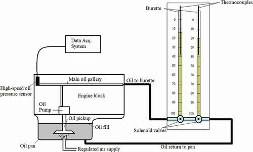
The oil pressure was used as the real-time indicator of oil aeration under the theory that more air trapped in the oil would lead to a greater degree of fluctuation and variance in the oil pressure as the oil was compressed by the oil pump. Besides its original functionality, the oil pump was essentially used as a testing device for oil aeration detection purpose. Therefore, a high-speed oil pressure sensor was mounted on the oil gallery passages closest to the oil pump outlet to record the engine oil pressure. Oil pressure data from the mounted sensor was recorded with high speed data acquisition system triggered by an engine mounted encoder. The resulting oil pressure was recorded in the data acquisition system with a constant 1 degree crank angle resolution, independent of the engine operating speed. Due to the fixed sampling rate of the data acquisition system in reference to the engine speed, this paper will refer to all frequency measurements in engine order as opposed the Hertz. An engine order of 1 signifies a frequency occurring once every rotation of the engine crankshaft. The data acquisition was conducted over 300 combustion cycles of the engine (each consisting of 720 degrees of crank angle rotation for a four-stroke engine) and the resulting signal was cycle-averaged in the crank angle domain to yield a single trace consisting of oil pressure measurements with 1 degree crank angle resolution over 720 crank angle degrees.

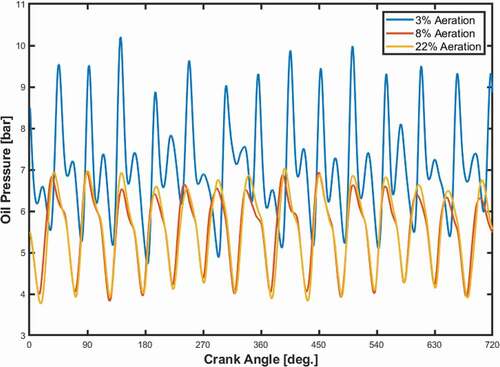
A sample of the averaged oil pressure traces recorded using the high-speed oil pressure sensor are shown in Figure 2. The traces show 14 distinct peaks as the 7 lobes of the engine oil pump, rotating at the same speed as the engine, pressurize the oil over two engine revolutions (720 degrees of crank angle). These pressure pulses contains useful information of oil aeration, as evidenced by the change in traces with changing oil aeration. However, the correlation between the traces is not straightforward. For example, a significant change is observed when aeration increases from 3% to 8% while further increase to 22% corresponds to a minute difference in the magnitude of the pressure pulses.

Figure 2. 300 cycle averaged oil pressure traces recorded by the high-speed oil pressure sensor in the crank angle domain with three different measured oil aeration.

For each oil pressure trace logged using the pressure sensor, the corresponding oil aeration was measured using the volume method by sampling oil from the engine oil gallery into a burette. The initial volume of the sample was recorded along with its temperature and atmospheric pressure and the oil sample was allowed to deaerate over thirty minutes. After this period of time, the final volume of the sample was also recorded with the corresponding temperature and atmospheric pressure. With these measurements, the oil aeration in the sampled oil-air mixture was calculated as the volume change of the sampled oil-air mixture and then corrected to standard temperature and pressure conditions to eliminate the influence of engine operating conditions. This was achieved using the following equations:

$Oilaeration=\frac{V_{air}}{V_{air}+V_{oil}}$

$V_{oil}=\frac{V_2}{1-{\alpha }_t\left(T_{ref}-T_2\right)}$

$V_{air}=\frac{P_{atm}{T}_{ref}\left(V_1-\frac{V_2}{1-\frac{{\alpha }_t}{\rho }\left({\mathrm{T}}_2-T_1\right)}\right)}{P_{ref}{T}_1}$

In these, V_air and V_oil refer to the volume of air and oil in the sample, respectively, corrected to a common reference temperature and pressure of T_ref and P_ref. These were calculated using V₁ and V₂, the volumes of the sampled oil at initial fill and after thirty minutes, T₁ and T₂, the temperatures of the sampled oil at initial fill and after thirty minutes, α_t, the coefficient of thermal expansion of the oil, ρ, the density of oil, and P_atm, the atmospheric pressure at the time of sampling. For this work, P_ref and T_ref were chosen as 101325 Pa and 373.15 K, and the density of oil and coefficient of thermal expansion were found to be 802.25 kg/m³ and 0.613 kg/(m³-K) from the manufacturer’s specifications.

A total of 134 averaged oil pressure traces and their corresponding oil aeration measurements using the volume method were collected in this manner for training the machine learning model. These were then divided into two sets: the first set consisting of 108 (80% of the total number of traces) randomly chosen traces was used in training the machine learning algorithm, while a second set of 26 (20% of the total number of traces) were reserved to validate the model and compare the performance of various machine learning hyper-parameters. These data sets were referred to as the training dataset and validation dataset, respectively. Besides these, an additional set of 12 oil pressure traces were collected from another engine of the same type in a different test room to test the performance of the machine learning model in eliminating setup related phenomenon from the learned oil aeration behavior. This set of 12 traces was referred to as the test dataset and served to independently test the performance of the machine learning model on previously unseen data.

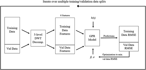
In order to extract the necessary features for training the machine learning model, each averaged oil pressure trace was analyzed with one-dimensional wavelet decomposition analysis. This decomposition analysis consisted of using five levels of cascading decomposition of the averaged oil pressure trace using a discrete wavelet transform (DWT). The DWT of a signal decomposes a signal by passing it through a pair of related high-pass and low-pass filters and then down-samples the result by a factor of two to generate a set of corresponding coefficients called the detail and approximation coefficients, respectively. These coefficients then represent the behavior of the input signal in the corresponding half (low or high) band of the input sampling frequency. In a cascading decomposition, each set of approximation coefficients then undergoes the DWT to generate a new pair of approximation and detail coefficients representing information on the signal in finer frequency bands. Figure 3 below illustrates this concept of a wavelet decomposition up to level three. Additional information about the DWT can be found in (Dghais and Ismail 2013).

Figure 3. Schematic of a three-level cascading DWT. g[n] and h[n] represent the corresponding low-pass and high-pass filters, respectively.

For the purposes of the oil aeration analysis described here, five levels of cascading DWT were undertaken to generate six corresponding sets of coefficients (five detail coefficients and one approximation coefficient at the fifth level). Each level of decomposition represented frequency content summarized in Table 1 below. The DWT decomposition was limited to five levels since the frequency content of the level five detail coefficients successfully captured the frequency content of the engine oil pump operating at a speed of 7 engine orders. The Daubechies 4 wavelets were used to generate the corresponding filters for this analysis as they were found to produce the best fit for the training and validation datasets.

Table 1. Frequency content of each level of DWT decomposition of the sampled oil pressure trace with sampling frequency f_s of 360 engine orders (1 degree sampling resolution)

Level	Coefficients	Frequency content
1	Detail	$\frac{f_s}{4}\mathrm{t}\mathrm{o}\frac{f_s}{2}$	90–180 Engine orders
2	Detail	$\frac{f_s}{8}\mathrm{t}\mathrm{o}\frac{f_s}{4}$	45–90 Engine orders
3	Detail	$\frac{f_s}{16}\mathrm{t}\mathrm{o}\frac{f_s}{8}$	22.5–45 Engine orders
4	Detail	$\frac{f_s}{32}\mathrm{t}\mathrm{o}\frac{f_s}{16}$	12.25–22.5 Engine orders
5	Detail	$\frac{f_s}{64}\mathrm{t}\mathrm{o}\frac{f_s}{32}$	6.13–12.25 Engine orders
5	Approx	$0\mathrm{t}\mathrm{o}\frac{f_s}{64}$	0–6.13 Engine orders

After generating the six sets of coefficients using the cascading DWT, the variance of each set was calculated using the formula:

$x=Var\left(C_i\right)=\frac{1}{n_i}\sum _{j=1}^{n_i}{\left(c_j-{\mu }_{Ci}\right)}^2;\mathrm{i}=1\dots 6$

where Var(C_i) is the variance of the DWT coefficients of set i (i ranges from 1 to 6 for the five detail and one approximation set of coefficients), n_i is the number of coefficients in set i, resulting from the DWT at that level, c_j are the individual coefficients in that set and µ_Ci is the arithmetic mean of that set of coefficients. This set of 6 variance values for the DWT coefficients was referred to as x, a vector of 6 values that together represented the oil aeration content for each oil pressure trace.

These six DWT variances for each recorded oil pressure trace were then fed into a Gaussian Process Regression (GPR) model as predictors along with the corresponding measured oil aeration values using the volume method as the expected response. The GPR model was then optimized using the training set of oil pressure traces to fit and predict the observed aeration to the recorded oil pressure trace.

A GPR model is a nonparametric model that calculates the probability distribution of parameters over all admissible functions that fit the data as it becomes available. It has the advantage of providing good fit over small datasets and allows good trade-off between fitting and smoothing based on the observed dataset. A more detailed analysis of GPR is presented in (Seeger 2004). For the oil aeration prediction, this GPR model used was of the form of

where y was the measured oil aeration i.e. the response, h(x) was a basis function to transform x, the set of six DWT variance-based predictors for each measured oil aeration y, β was a vector of coefficients for the basis function transformation and, f(x) was a variable introduced for the GPR model to capture the variance in the six predictors in the training dataset. This latent variable f(x) was chosen such that the set of all f(x) for each recorded oil measurement y formed a Gaussian distribution with a mean of 0 and a covariance defined by a Kernel function k(x,x’). In mathematical terms,

$f\left(x\right)\sim \mathcal{N}\left(0,k\left(x,x{ }^{\mathrm{\prime }}\right)\right)$

With this model, the response of the GPR model was expressed using the probability function:

$P\left(y|x,f\left(x\right)\right)\sim \mathcal{N}(y|h\left(x\right)\beta +f\left(x\right),{\sigma }^2)$

Thus, using the GPR model, the probability of each measured oil aeration could be expressed using a Gaussian distribution function with a mean equal to a transformation of the observed DWT features and their covariance and a standard deviation σ, that captured the inherent system noise during the measurement process. The GPR model then optimized the values of σ and β to minimize the difference in the predicted response and the observed values. h(x) and k(x) are left as hyperparameters for the model to be adjusted to improve fit.

For the oil aeration modeling, only the hyperparameter h(x) was optimized to improve the model fit. The hyperparameter f(x) kernel function was kept constant for this model to reduce computation effort and took the form of the ‘rational quadratic’ kernel function listed in (Rasmussen and Williams 2006). The options examined for the hyperparameter options for the basis function h(x) are listed below in Table 2.

Table 2. Basis functions h(x) explored for GPR model hyperparameter optimization

Basis function	h(x)
None	$h\left(x\right)=0$
Constant	$h\left(x\right)=1$
Linear	$h\left(x\right)=x+1$
Quadratic	$h\left(x\right)=x^2+x+1$

For each basis function, the optimal σ and β were calculated initially using the training data and then refined through iteration to minimize the root-mean-squared error (RMSE) on the validation dataset. To observe the effect of the training/validation data split on the resulting optimization, this entire optimization process was repeated multiple times using additional random training/validation data splits. The basis function that yielded the lowest average validation RMSE over these multiple training/validation splits was chosen as the optimal model for oil aeration prediction. A summary of the overall process used to develop the trained model is shown below in Figure 4.

Figure 4. Schematic of the training process for the GPR model for oil aeration predictions. Note that h(x) is a hyperparameter of the model and is fixed during each iteration.

After training the model to minimize the prediction RMSE on the validation dataset, the final set of 12 oil pressure traces was fed into the model as an independent verification of the model on previously unseen data. Like the training and validation data, six DWT predictors were extracted from these 12 traces and this set of predictors was fed into the GPR model with optimal h(x), σ and β as determined from the training process. The predictions from the model were then used to calculate the RMSE error on the test set to characterize the performance of the model.

Results

Using the above methodology, the trained GPR model with the six variance-based features of the five-level DWT decomposition contained the following parameters listed in Table 3.

Table 3. Parameters of optimized GPR model

Parameter	Value
$\beta$	$0.0830$
$\sigma$	$0.0142$
$h\left(x\right)$	Constant; $h\left(x\right)=1$
Mean Val. RMSE	0.0157

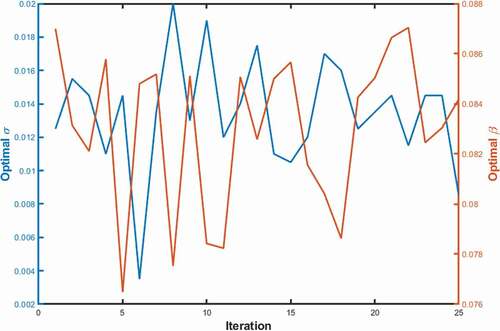
During the optimization process, the optimal sigma for the GPR model was found to be heavily dependent on the training/validation data split and tended to vary depending on the random distribution of oil pressure traces into the training or validation data sets. An example of this dependence is shown below in Figure 5 for a series of iterations using randomly divided training and validation data sets. Hence, to minimize the effect any training data bias, 25 random training/validation splits were run and the optimal values of σ and β were averaged over each iteration to give an overall optimal set of parameters for the model. As a result of the averaging process, these averaged parameters were not optimal for any one training/validation split but instead minimized the error given any randomly assigned data distribution.

Figure 5. Variation in optimal σ and β of GPR model based on training/validation data split.

Using this averaging concept to reduce the dependence on training/validation data split, the hyperparameter h(x) was optimized for this model by running 25 iterations of various training/validation data splits for each basis function and calculating the resulting validation data RMSE as shown in Figure 4. To get an estimate of the performance of each basis function, the results of the 25 iterations were then averaged into a representative value for that basis function. The results of these iterations are shown below in Figure 6 and the averaged values for each function are summarized in Table 4.

Table 4. Mean of GPR model parameters for each basis function over 25 iterations of training/validation data split. Note that β is a vector of coefficients for the basis function h(x) and x is a vector of six DWT-based variances for each observation y.

Basis function	Mean of optimal β	Mean of optimal σ	Mean validation RMSE
h(x) = 0	-	0.0156	0.0164
h(x) = 1	0.0830	0.0142	0.0157
h(x) = x + 1	βl	0.0129	0.0186
h(x) = x^2 + x + 1	βq	0.0119	0.0221

β_l = [0.0744, 0.00985, 0.0146, −0.0188, 0.0193, −0.0131, −0.0113]

β_q = [0.0554, 0.0185, 0.0181, −0.0211, −0.0134, −0.0024, −0.0656, 0.0014, – 0.0055, 0.0012, 0.0110, 0.0037, 0.0109]

Figure 6. RMSE of oil aeration predictions on the validation dataset over multiple iterations of training/validation data split.

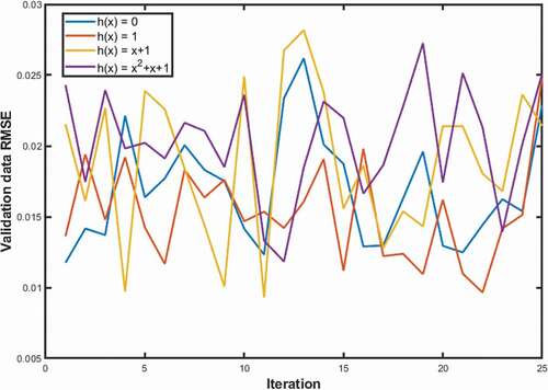
From these results, it was observed that the hyperparameter h(x) = 1, i.e. the constant basis function, on average, resulted in the best prediction accuracy in the model and hence the parameters for this model were chosen as the optimized parameters of the GPR model as previously shown in Table 3.

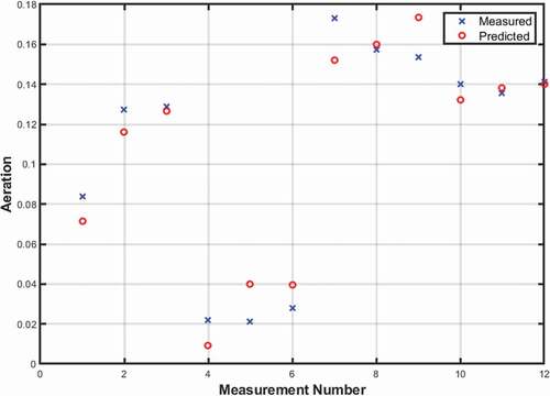
Finally, this GPR model with the optimized parameters was used with the 12 oil pressure traces from the test dataset to determine its effectiveness on previously unseen data. The overall prediction performance and the accuracy of predictions on the test dataset are shown below in Figure 7 and Figure 8, respectively. The RMSE values of this model are summarized in Table 5. Thus, the optimized GPR model with parameters shown in Table 3 was able to fit the training data with a RMSE of 0.0129 from the measured oil aeration value using the volume method. Furthermore, for the validation data, the same model yielded an RMSE of 0.0157 from the measured oil aeration and an RMSE of 0.0121 on the 12 independent oil pressure traces sampled to test the model. The similarity in fit between the training, validation, and test data sets indicates good fit of this model and excludes potential overfitting or underfitting issues and demonstrates that the trained model is successfully able to predict oil aeration by recording fluctuations in engine oil pressure alone.

Table 5. Performance of optimized GPR model

	Optimized GPR model
Training data RMSE	0.0129
Validation data RMSE	0.0157
Test data RMSE	0.0121

Figure 7. Performance of the GPR model with the training, validation, and test datasets compared to an ideal model fit.

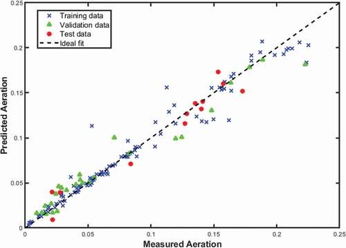
Figure 8. Optimized GPR model predictions with on the test data compared to measured aeration.

Practical Considerations

The machine learning method presented here shows good success in detecting oil aeration using only a high-speed oil pressure sensor and this method has the potential for implementation in real-time monitoring oil aeration in vehicle. However, in-vehicle recordings of oil pressure may have to make use of lower resolution data than 1 degree of crank angle, especially if a high-resolution encoder cannot be easily mounted on the engine due to space constraints and data must instead be collected using existing engine signals such as crank rotation sensors or flywheel rotation sensors.

To test the effects of such signals on the model, the collected signals were downsampled to a resolution of 3 and 6 degrees of angular resolution. The training and validation datasets were then fed into the process shown in Figure 4 and Table 3. No hyperparameter optimization was conducted for this investigation and the previously found constant basis function h(x) was used. With this model, the previous analysis was repeated and the GPR model was found to have the following characteristics shown in Table 6. The predictions made by the model for the 3 degree resolution data are shown in Figure 9 and Figure 10 and the model predictions for the 6 degree resolution data are shown Figure 11 and Figure 12.

Table 6. Performance of GPR model on downsampled oil pressure traces

	1 degree sampling	3 degree sampling	6 degree sampling
Training data RMSE	0.0129	0.0075	0.0060
Validation data RMSE	0.0157	0.0171	0.0238
Test data RMSE	0.0121	0.0179	0.0240

Figure 9. Performance of the GPR model with the training, validation and test datasets compared to an ideal model fit for oil pressure traces sampled at 3 degrees resolution.

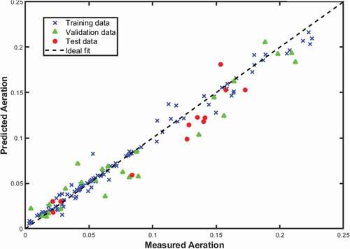
Figure 10. GPR model predictions with on the test data compared to measured aeration using oil pressure traces sampled at 3 degrees resolution.

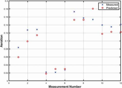
Figure 11. Performance of the GPR model with the training, validation, and test datasets compared to an ideal model fit for oil pressure traces sampled at 6 degree resolution.

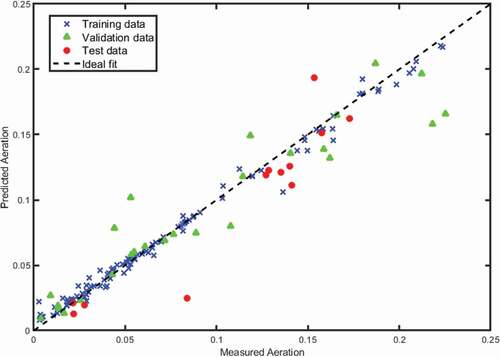
Figure 12. GPR model predictions with on the test data compared to measured aeration using oil pressure traces sampled at 6 degrees resolution.

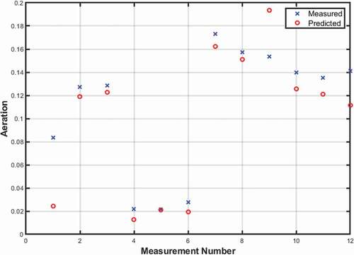
In both cases, the downsampled data resulted in worse aeration predictions from the model compared to the 1 degree resolution data. Both cases also demonstrated a degree of overfitting, as the training data showed low RMSE, while the validation and test datasets showed similar and higher prediction RMSE. These results indicate that the lower sampling resulted in the model learning the behavior of training data to a greater degree rather than the characteristics of the oil aeration in the training data.

However, despite the poorer fit, the 3 degree resolution model was still able to accurately predict the oil aeration in the test data with an error of approximately ± 0.02 from the measured aeration values. Even the 6 degree resolution model was able to predict the oil aeration in the test data with an error very close to ± 0.02 for 10 out of the 12 test data points. For engine design or diagnostic cases, such an error may be acceptable, especially during stages where engine components are being iteratively tested to see if they qualitatively reduce oil aeration. The greater uncertainty in the oil aeration predictions of the lower resolution models can also be mitigated by making several predictions using the model at the same operating point, thus getting a better idea of the true oil aeration condition of the engine.

Thus, the presented model can provide an acceptable method of predicting oil aeration even when the oil pressure data is sampled at resolutions as low as 6 degrees of crankshaft rotation.

Conclusion

This research work develops a machine learning model for intelligent detection and real-time monitoring of oil aeration using only high-speed engine oil pressure recordings. This method has the advantage of monitoring and predicting the oil aeration conditions of an engine online and in-vehicle without the need for specialized test equipment. Once trained using previous oil pressure data, this method was successfully able to predict the engine oil aeration with an uncertainty of under ±0.02 from the measured oil aeration values. Furthermore, while the method was found to work best when used with oil pressure data sampled at 1 degree crank angle resolution, investigating its sensitivity to sampling rate found that it may produce acceptable results with sampling resolutions as low as 6 degrees.

Disclosure Statement

No potential conflict of interest was reported by the author(s).

References

- Baran, B. A. 2007. engine lubrication oil aeration. Cambridge: Massachusetts Institute of Technology.
- Bregent, R. L., P. A. Porot, E. A. Monchaux, and J. M. Cailliez. 2000. “The SMAC, under pressure oil aeration measurement system in running engines.” SAE technical paper No. 2000–01-1818.
- Deconninck, B., T. Delvigne, and G. Videx. 2003. “Air-X, and innovative device for online oil aeration measurement in running engines.” SAE technical paper no. 2003-01-1995.
- Dghais, A., and M. Ismail. 2013. A comparative study between discrete wavelet transform and maximal overlap discrete wavelet transform for testing stationarity. International Journal of Mathematical and Computational Sciences 7 (12):1677–81.
- Kateris, D., D. Moshou, X.-E. Pantazi, I. Gravalos, N. Sawalhi, and S. Loutridis. 2014. A machine learning approach for the condition monitoring of rotating machinery. Journal of Mechanical Science and Technology 28 (1):61–71. doi:https://doi.org/10.1007/s12206-013-1102-y.
- Koch, F., T. Hardt, and F. Haubner. 2001. “Oil aeration in combustion engines – analysis and optimization.” SAE Paper No. 2001-01-1074.
- Li, Q., C. Rajagopalan, and G. D. Clifford. 2014. A machine learning approach to multi-level ECG signal quality classification. Computer Methods and Programs in Biomedicine 117 (3):435–47. doi:https://doi.org/10.1016/j.cmpb.2014.09.002.
- McComb, N., and A. Cooper. 2003. “A new technique for dynamic oil aeration monitoring.” SAE Paper 2003-01-1994.
- Morgan, C., J. Cummings, R. Fewkes, and J. Jackson. 2004. “A new method of measuring aeration and deaeration of fluids.” SAE Paper No. 2004-01-2914.
- Qiao, X., L. Pengfei, J. Bai, J. Zhuang, and Z. Huang. n.d. “Oil aeration measurement on a high-speed diesel.”
- Rasmussen, C. E., and C. K. Williams. 2006. Gaussian processes for machine learning. Cambridge, Massachusetts: MIT Press.
- Seeger, M. 2004. Gaussian processes for machine learning. International Journal of Neural Systems 14 (2):69–106. doi:https://doi.org/10.1142/S0129065704001899.