Strip Steel Defect Classification Using the Improved GAN and EfficientNet

ABSTRACT

In recent years, deep-learning detection algorithms based on automatic feature extraction have become the focus of defect detection. However, limited by industrial field conditions, the insufficient number of images in the collected dataset restricts the detection effect of deep learning. In this paper, an algorithm of strip steel defect classification using the improved GAN and EfficientNet was proposed. First, the label deconvolution network is constructed, where the image labels were deconvolved layer by layer to obtain the conditional masks that were superimposed into the generator and discriminator to form Mask-CGAN. Then, the mode-seeking generative adversarial networks (MSGAN) were improved and used to solve the problem of mode collapse. Finally, the EfficientNet was improved and trained on the dataset expanded by Mask-CGAN, which achieved the classification of strip steel defects. Experiments showed that Mask-CGAN proposed in this paper can generate true-to-life images and solve the problem of insufficient samples in deep learning. The improved EfficientNet with fewer parameters can accurately and efficiently classify strip steel defects.

Introduction

Strip steel is one of the important raw materials in automotive, marine, aerospace, and other industries. The quality of strip steel directly affects the final performance of industrial products. In the production process of strip steel, various defects such as holes, scratches, rolling, cracks, and pits will occur due to different raw material sources, different processing techniques, and different rolling equipment (Neogi, Mohanta, and Dutta 2014). These defects in strip steel not only affect the appearance but also reduce the wear resistance, corrosion resistance, fatigue resistance, and other physical properties of industrial products, thus leading to the existence of huge potential safety hazards in industrial products. Therefore, it is of great significance to study the defect detection of strip steel.

In recent years, the performance of deep learning in the field of image recognition is getting higher and higher (Kiani, Keshavarzi, and Bohlouli 2020; Yang et al. 2019; Zhuang et al. 2019). In this paper, deep learning was used to classify strip steel defects. However, there are few samples of strip steel defect dataset, which brings difficulties to the training of deep learning. Therefore, an algorithm of strip steel defect classification using the improved GAN and EfficientNet was proposed in this paper. Firstly, in order to generate various kinds of strip steel defect images, the image generation model GAN was improved. The label deconvolution network was constructed and integrated into the generator and discriminator to form Mask-CGAN. In order to solve the problem of mode collapse, the mode-seeking generative adversarial networks (MSGAN) were introduced and improved. Then, strip steel defect images were generated by Mask-CGAN and used to expand the dataset. Finally, in order to improve the accuracy and real-time of strip steel defect classification, the image classification network EfficientNet was improved and trained on the expanded dataset.

China is the world’s largest manufacturing country, China’s industrial products production in the world’s first 220 kinds of production, including crude steel production has been the world’s first for many years, in 2020 China’s total crude steel production accounted for 57% of the world, of which strip steel production has been accounting for most of the total production, has reached 50% of the total production. With the rapid progress of national modernization and the increasing consumption level of downstream users, the demand for strip steel is also increasing, which also puts forward higher requirements on the quality of strip steel products. Therefore, the research on the defect detection of strip steel is of great significance. It can help manufacturers to better grasp the quality of their products, to separate them according to different quality levels, to provide downstream users with products that meet their quality requirements, to establish the image and reputation of strip steel producers, and to reflect the image of a manufacturing power. The contributions of this research work are as follows:

The image labels were deconvoluted layer by layer to form the label deconvolution network, which was integrated into GAN to generate various kinds of strip steel defect images.

The image similarity calculation of MSGAN was transferred from image space to feature space, which made the similarity calculation more robust. The improved MSGAN was used to solve the problem of mode collapse.

This paper improved EfficientNet so that its parameter amount and predicted time were greatly reduced, which can accurately and efficiently classify strip steel defects.

The structure of the rest of this paper is as follows: Section 2 introduces the related works of strip steel defect detection and GAN. Section 3 introduces the improved EfficientNet and the improved GAN respectively. Section 4 contains the experimental results and analysis of GAN training and strip steel defect classification. Section 5 summarizes the work of this paper and looks forward to the future research.

Related Works

Manual detection of strip steel defects is easily affected by experience and subjective factors, and the detection efficiency is low, so it is difficult to meet the needs of online detection. With the development of machine vision, various detection algorithms based on machine vision have been widely used in strip steel defect detection. Sharifzadeh et al. (2008) used image processing algorithm to detect four kinds of common strip steel defects, with an accuracy of 90%. Ghorai et al. (2013) proposed a defect segmentation method based on texture threshold. The problem of low detection rate of small defects on strip steel surface was solved by extracting the wavelet features of image area by block. Aghdam and Amid (2012) extracted LBP features of strip steel defect image and classified them by decision tree, and achieved good results. Guan (2015) achieved the image segmentation of strip steel defects by constructing saliency maps. Jiawei Zhang, et al. (2020) estimated the degree of defects in each gray level of strip images by membership function, and used the maximum value of fuzzy connected area to locate defects, with detection accuracy as high as 96.8%. HuaiLiang Zhang et al. conducted preliminary detection of surface defects of ceramic tiles by significance, and then conducted secondary detection of image sub-blocks of defect areas, with the final detection accuracy up to 98.75%. The feature extraction of classical algorithm for strip steel defect detection is based on the artificial experience. However, it is difficult to obtain the detection methods matching with strip steel by using the artificial experience. How to automatically extract features to adapt to different types of defect detection has become an urgent problem.

Deep learning can automatically learn image features and its performance in many fields is significantly higher than traditional algorithms. In recent years, more and more researchers have introduced deep learning to solve the detection problem that traditional machine vision is difficult to solve (Haselmann and Gruber 2019; Lin et al. 2020; Wang and Guan 2017). Park et al. (2016) established and tested several depth networks with different depth and layer node number to select the appropriate network structure for surface defect detection. Faghih-Roohi et al. (2016) classified five kinds of rail defects by convolution neural network, with the highest accuracy of 93.04%. Youkachen et al. (2019) realized image segmentation of strip steel defects through convolution automatic encoder and convolution image processing. He et al. (2020) used multilevel feature fusion network and region proposal network to detect strip steel defects, with an accuracy of 92%. Xinglong Feng, Gao, and Luo (2021) proposed the RepVGG algorithm and its combination with the spatial attention mechanism, and the accuracy of the algorithm reached 95.10%. Sebastian Meister, Mahdieu Wermes et al. (2021) proposed a parallel classification method for convolutional neural networks (CNN) and support vector machines, with an average classification rate of 86.0% for convolutional neural networks (CNN) and up to 70% for support vector machines. The deep learning algorithms trained on many samples can effectively solve the problem of defect detection. Due to the constraints of industrial field data collection conditions and data collection costs, the number of samples in the dataset often cannot meet the needs of training, which leads to problems such as underfitting and affects the detection effect. How to expand the dataset with few samples needs further study (Perez and Wang 2017).

Goodfellow et al. (2014) proposed a generative adversarial network (GAN) model, which includes generator and discriminator. The generator tries to generate fake images that deceive the discriminator. The discriminator tries to distinguish between real and fake images. The generator and discriminator continuously conduct confrontation training. Finally, the generator can generate some true-to-life samples according to the characteristics of the original data. Mirza and Osindero (2014) proposed conditional generative adversarial networks (CGAN), which can generate various kinds of images at the same time. Radford, Metz, and Chintala (2016) introduced convolutional neural networks into GANs and proposed deep convolutional generative adversarial networks (DCGAN), which laid the foundation for generating higher resolution images. In recent years, many scholars have used GANs to expand datasets and achieved good results. Frid-Adar et al. (2018) used GANs to generate calculated topography images to expand the dataset, which increased the specificity from 88.4% to 92.4%. Xuan et al. (2019) used GAN to generate multi-view pearl images, and trained multistream structural network on the expanded dataset to significantly reduce the error of pearl classification. Yi and Cho (2020) used GAN to expand the pedestrian detection dataset and achieved good results. Sebastian Meister, Nantwin Moller et al. (2021) show that a conditional deep convolutional generative adversarial network combined with a previous geometric transformation is well suited to generate a large realistic dataset from less than 50 actual input images.

Proposed Method

The Improved EfficientNet

In this paper, image classification network in deep learning was used to realize strip steel defect classification. Some classic image classification networks can achieve high accuracy by increasing the network depth and other operations that complicate the network. However, the complex network structure will lead to too many parameters, take up a lot of memory, and slow prediction speed. In recent years, many scholars began to study lightweight neural networks (Howard et al. 2017; Zhang et al. 2018). On the premise of high accuracy, the network architecture was simplified as much as possible, so that it can run in devices with limited performance such as mobile phones.

While classical classification networks are usually deflated by one dimension to achieve higher accuracy, the Lightweight Neural Network EfficientNet (Tan and Le 2019) searches for the optimal network architecture by adjusting the depth, width, and resolution of the network, comprehensively considering the accuracy and real-time. The author of EfficientNet first obtained the baseline network through the network structure search, that is, EfficientNet-B0, and then scaled it in the three dimensions of depth, width, and resolution to obtain a series of models from EfficientNet-B1 to EfficientNet-B8. From B0 to B8, the number of parameters gets larger and larger, and the accuracy gets higher and higher. The image classification performance of EfficientNet is better than most existing image classification networks, and the improved EfficientNet lightweight network is compared with the classical image classification network, the original EfficientNet, and the original ShuffleNetV2 lightweight classification network, respectively. The results are shown in Table 3. The improved EfficientNet network in this paper has fewer parameters and faster prediction speed, which can meet the requirements of industrial applications. Therefore, EfficientNet is used to classify strip defects in this paper.

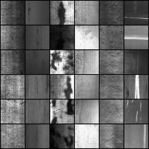
The original strip steel defect dataset contains six kinds of defects, each kind of defect contains 300 images, each image is a gray image with a resolution of 64 × 64. Some examples of the original strip steel defect images are shown in Figure 1. Each column is a kind of strip steel defect, the first column is the crazing defect, the second column is the inclusion defect, the third column is the patch defect, the fourth column is the pitted surface defect, the fifth column is the rolled in scale defect, and the sixth column is the scratch defect.

Figure 1. Some examples of the original strip steel defect images.

The original EfficientNet was trained on the ImageNet dataset containing color images with a resolution of 224×224. The strip steel defect images used in this paper are much less complex and much less difficult to identify, so EfficientNet-B0 with low parameter quantity was used. For the convenience of expression, EfficientNet mentioned below refers to EfficientNet-B0. The original EfficientNet was improved to reduce the number of parameters and increase the operation speed, which is more suitable for the classification of strip steel defects.

Reference the original EfficientNet show way, the structure of the improved EfficientNet is shown in Table 1. “Resolution” is the input resolution, and “Channels” is the number of output channels. Some redundant structures of the original EfficientNet were removed on the premise of retaining the key modules. For example, the out channels in the penultimate row of Table 1 were changed from 1280 to 240. MBConv6 layers were deleted and two layers of MBConv5 were added. Other improvements in Table 1 can be compared in detail with the original EfficientNet.

Table 1. Structure of the improved EfficientNet

Stage	Operator	Resolution	Channels	Layers
1	Conv3x3	64x64	16	1
2	MBConv1, k3x3	32x32	48	2
3	MBConv5, k5x5	16x16	72	2
4	MBConv5, k5x5	8x8	96	1
5	Conv1x1 & Pooling	8x8	240	1
6	Full Connection	1	6	1

The original strip steel defect dataset contains six kinds of defects, each kind of

defect contains 300 images. The original strip steel defect dataset was divided into training set and testing set. Each kind of defect in the training set contained 200 images, and each kind of defect in testing set contained 100 images. The test set was only used for evaluation and did not participate in neural network training. The improved EfficientNet was pre-trained on the train set. After 100 epochs, the accuracy on the test set reached 90.02%, which initially proved the effectiveness of the improved EfficientNet in strip steel defect classification. More complete experiments will be done in section 4.

The Improved GAN

In order to expand the strip steel defect dataset, an improved GAN model combining conditional control advantage of CGAN with convolution advantage of DCGAN was proposed in this paper, which can generate various kinds of strip steel defect images. Firstly, the label deconvolution network was constructed, and the image labels were deconvoluted layer by layer to get the feature maps of different sizes, which were called conditional masks. Then, the conditional masks and the feature maps of the corresponding size in the generator of DCGAN were superposed. Finally, the conditional masks and the feature maps of the corresponding size in the discriminator of DCGAN were superposed. In this way, Mask-CGAN was formed. The specific training flow chart is shown in Figure 4, which also reflects the novelty of combining a supervised deep learning model with an unsupervised GAN model. This part first introduces the label deconvolution network, then analyzes the generator network and the discriminator network in detail.

The Label Deconvolution Network

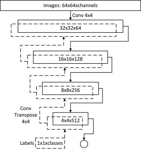
The structure of the label deconvolution network is shown in the dotted line part of Figures 2 and 3. “Labels” refers to image tags, and “classes” refers to the number of image categories. “Conv transpose 4 × 4” refers to the deconvolution operation with the convolution kernel size of 4 × 4. All dashed arrows are deconvolution operations of the label deconvolution network. “4 × 4x512” refers to the size of a set of feature maps, “4 × 4” refers to the width and height, respectively, “512” refers to the number of channels, and so does other similar texts such as “8 × 8 x 256.” The “Mask” in Mask-CGAN refers to the conditional masks, that is, the feature maps of different sizes (dotted boxes in Figures 2 and 3) obtained through the label deconvolution network.

Figure 2. Generator network structure.

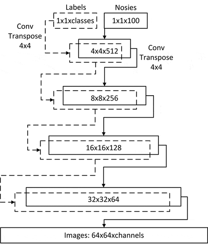
Figure 3. Discriminator network structure.

First, the original image labels are encoded by one-hot to get 1 × 1 x classes image labels. There are six kinds of strip steel defect images, so “classes” is 6. Then, the image labels are deconvoluted to obtain 4 × 4 x 512,8 × 8 x 256,16 × 16 x 128,32 × 32 x 64 conditional masks in turn. The activation function of each layer of the label deconvolution network is LeakyReLU. Except for the input layer, the other layers are processed by batch normalization.

The Generator Network

The generator network structure is shown in Figure 2. “Noises” in Figure 2 refers to a group of random numbers that follow a standard normal distribution, also called Gaussian white noise. “Conv transpose 4 × 4” refers to the deconvolution operation with the convolution kernel size of 4 × 4. The solid arrows in Figure 2 are all deconvolution operations. “Channels” refers to the number of channels of the final generated images. The generator is mainly composed of the noise deconvolution network (solid-line part in Figure 2) and the label deconvolution network (dotted line part in Figure 2). The inputs of the generator are random noises and image labels, and the outputs are images with resolution of 64 × 64. The strip steel defects to be generated are grayscale images, so “channels” is 1. The specific steps of the generator operation are as follows:

The input random noises are deconvolved into 4 × 4 × 512 feature maps, and then added to the corresponding size of conditional masks and deconvolved to obtain 8 × 8 × 256 feature maps.

The 8 × 8 × 256 feature maps are added to the corresponding size of conditional masks and deconvolved to obtain 16 × 16 x 128 feature maps.

The 16 × 16 × 128 feature maps are added to the corresponding size of conditional masks and deconvolved to obtain 32 × 32 × 64 feature maps.

The 32 × 32 × 64 feature maps are added to the corresponding size of conditional masks and deconvolved to obtain the generated images of 64 × 64 × channels.

Other important configurations of the generator network are as follows: except for the Tanh activation function of the output layer, the activation function of the other layers is LeakyReLU. Except for the input layer and the output layer, the other layers are processed by batch normalization to speed up convergence.

Ideally, when the same image labels and different random noises are input to the generator, the strip steel defect images with slightly different features will be generated. But in actual training, GAN is prone to mode collapse. When the same image labels and different random noises are input, the generated images are very similar. Mode collapse can reduce the diversity of the generated samples and even cause image distortion. Mao et al. (2019) conducted research from this perspective and proposed mode seeking generative adversarial networks (MSGAN). As shown in Equation (1)(1) $L_{\mathrm{n}\mathrm{e}\mathrm{w}}=L_{\mathrm{o}\mathrm{r}\mathrm{i}}+{\lambda }_{ms}{L}_{ms}$(1) , MSGAN adds a mode seeking loss (L_ms) to the loss function of the generator. L_ms is shown in Equation (2)(2) $L_{ms}=\underset{G}{max}\left(\frac{d_I\left(G\left(c,z_1\right),G\left(c,z_2\right)\right)}{d_z\left(z_1,z_2\right)}\right)$(2) .

(1) $L_{\mathrm{n}\mathrm{e}\mathrm{w}}=L_{\mathrm{o}\mathrm{r}\mathrm{i}}+{\lambda }_{ms}{L}_{ms}$(1)

where λ_ms is the custom weight and L_ori is the original loss of the generator.

(2) $L_{ms}=\underset{G}{max}\left(\frac{d_I\left(G\left(c,z_1\right),G\left(c,z_2\right)\right)}{d_z\left(z_1,z_2\right)}\right)$(2)

where G refers to the generator, c refers to the image labels, and z₁ and z₂ refer to two sets of random noises. d_I refers to the L1 distance of two groups of images, and d_z refers to the L1 distance of two groups of random noises. The optimization goal of L_ms is to maximize the ratio of the distance between G(c, z₁) and G(c, z₂) with respect to the distance between z₁ and z₂.

MSGAN encourages the generator to generate diversified images to avoid mode collapse through L_ms, which has a good effect. But there is one detail that can be improved. MSGAN judges the similarity of two groups of images by calculating L1 distance in image space, which is easily interfered by background, brightness, and other factors. For example, the features of two groups of images are very similar, but one group of images is generally bright, and the other group of images is generally dark. In this case, the diversity is not ideal, but it is difficult to distinguish in the image space. Therefore, this paper proposed to judge the similarity of two groups of images in the feature space. The convolution neural network is used to extract the feature maps of the two groups of images, and then the L1 distance of the two groups of feature maps is calculated. The improved L_ms is shown in Equation (3)(3) $L_{ms}=\underset{G}{max}\left(\frac{d_F\left(G\left(c,z_1\right),G\left(c,z_2\right)\right)}{d_z\left(z_1,z_2\right)}\right)$(3) .

(3) $L_{ms}=\underset{G}{max}\left(\frac{d_F\left(G\left(c,z_1\right),G\left(c,z_2\right)\right)}{d_z\left(z_1,z_2\right)}\right)$(3)

where d_F denotes the L1 distance between two groups of images in the feature space.

The first part of this section has completed the improvement and pretraining of EfficientNet. Although the sample number of test set used in the pretraining is not large, after the test in this paper, the EfficientNet after the pretraining is enough to extract the feature maps of strip steel defects. When comparing image similarity in feature space, if the size of feature maps is too large, it will inevitably be mixed with background and other interference factors. If the size is too small, it cannot reflect the defect features. Therefore, the 16×16 feature maps of the images are extracted by the pretrained EfficientNet, and then the similarity of the two groups of images is judged in the feature space.

The Discriminator Network

The discriminator network structure is shown in Figure 3. “Conv 4 × 4” refers to the convolution operation with a convolution kernel size of 4 × 4. The discriminator is mainly composed of the image convolution network (solid-line part in Figure 3) and the label deconvolution network (dotted line part in Figure 3). The inputs of the discriminator are images with a resolution of 64 × 64 and image labels, and the outputs are floating values representing the result of the discrimination. The specific steps of the discriminator operation are as follows:

1. The input images are convoluted into 32 x 32 x 64 feature maps, and then added with the corresponding size of conditional masks and convoluted to obtain 16 × 16 x 128 feature maps.

The 16 ×16 x 128 feature maps are added to the corresponding size of conditional masks and convoluted to obtain 8 × 8 x 256 feature maps.

The 8 × 8 x 256 feature maps are added to the corresponding size of conditional masks and convoluted to obtain 4 × 4 x 512 feature maps.

The 4 × 4 x 512 feature maps are added to the corresponding size of conditional masks and convoluted to obtain the discrimination results.

Other important configurations of the discriminator network are as follows: except for the Sigmoid activation function of the output layer, the activation function of the other layers is LeakyReLU. Except for the input layer and the output layer, the other layers are processed by batch normalization to speed up convergence.

Results and Analysis

All the experiments of this section were completed on the same server. The main configuration is as follows: CPU is i7-7820x, graphics cards are two Geforce RTX 2080Ti, operating memory is 32 G, 512 G solid-state hard disk.

This section is divided into two experiments, the parameters used in the GAN image generation experiment and the classification experiment are shown in Table 2.

Table 2. Experimental parameter setting

Networks	Batch size	Optimizer	Learning rate	Training epochs
GAN series of image generation experiments	64	Adam	0.0002	500
Defect classification experiment	64	SGD	0.1	100

Table 3. Image classification of different networks

Networks	Parameter amount (millions)	Predicted time (ms)	Accuracy (%)	F1 score
ShuffleNetV2	1.29	302	93.00	0.93
The original EffieientNet	4.01	292	92.05	0.92
The improved EffieientNet	0.22	231	95.50	0.95
VGG16	17.35	327	93.81	0.94
ResNet34	21.28	323	91.16	0.91
DenseNet121	6.95	320	94.24	0.94

GAN Training Effect Analysis

In this paper, MSGAN was improved and used to solve the problem of mode collapse. Its specific training flow chart is shown in Figure 4. In the original MSGAN, the image similarity calculation is in the image space, and the improved one is in the feature space. In order to verify which space is more suitable for image similarity calculation, the L_ms is removed from the generator loss function, and then the Mask-CGAN is trained for 500 epochs, and L_ms is calculated according to Equations (2(2) $L_{ms}=\underset{G}{max}\left(\frac{d_I\left(G\left(c,z_1\right),G\left(c,z_2\right)\right)}{d_z\left(z_1,z_2\right)}\right)$(2) ) and (3(3) $L_{ms}=\underset{G}{max}\left(\frac{d_F\left(G\left(c,z_1\right),G\left(c,z_2\right)\right)}{d_z\left(z_1,z_2\right)}\right)$(3) ) every 10 epochs, respectively. Finally, the line graph shown in Figure 5 was obtained. In Figure 5, the dotted line represents the image space, and the solid line represents the feature space. The vertical coordinate loss (L_ms) in Figure 5 is equivalent to the evaluation index of the diversity of the generated images. The lower the L_ms, the stronger the diversity.

Figure 4. Training flow chart.

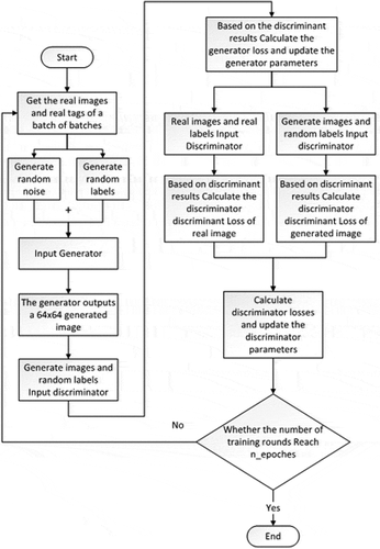
Figure 5. Mode seeking losses in different spaces.

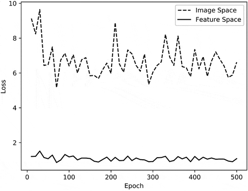
In general, the fluctuation trend of L_ms curve in image space and feature space is basically consistent. However, the overall L_ms curve in the image space is much higher than the feature space. L_ms in the feature space fluctuates around 1 with a small fluctuation range, and L_ms in the image space fluctuates around 7 with a large fluctuation range. Corresponding L_ms curve to the actual images, when the diversity of the generated images is poor or good, it can be indicated in both image space and feature space. When the diversity of the generated images is general, the indication of feature space is stable, while the indication of image space fluctuates greatly. This is because the calculation of similarity in image space will be interfered by background, brightness and other factors, resulting in larger losses and fluctuation. In a word, it is more robust to calculate image similarity in feature space.

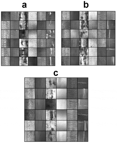
After verifying the effectiveness of the improved MSGAN, the L_ms of Equation (3)(3) $L_{ms}=\underset{G}{max}\left(\frac{d_F\left(G\left(c,z_1\right),G\left(c,z_2\right)\right)}{d_z\left(z_1,z_2\right)}\right)$(3) is multiplied by the weight λ_ms and added to the loss function of the generator. λ_ms is set to 1.0 with reference to the original MSGAN. The original strip defect image is shown in Figures 1, 6(a,b and c) are image generation results of the 100th, 300th, and 500th epochs of Mask-CGAN training, respectively. From the 100th to the 500th epoch, the image generation effect is getting better and better and the model has converged by the 500th epoch. That is to say, Figure 6(c) is the final image generation effect of Mask-CGAN, which is very close to the original images of Figure 1. Therefore, the Mask-CGAN proposed in this paper is suitable for expanding strip steel defect dataset.

Figure 6. Some examples of Mask-CGAN training process.

Strip Steel Defect Classification Effect Analysis

Based on 200 images of each defect in the training set, 1000 images of strip steel defects are generated by using the trained Mask-CGAN. The expanded training set contains 1200 images for each defect, while the test set still contains 100 images for each defect. In order to verify the effectiveness of the improved EfficientNet in strip steel defect classification, the original EfficientNet, the improved EfficientNet, VGG16, ResNet34, and DenseNet121 were used to train 100 epochs on the dataset expanded by Mask-CGAN. Except the networks are different, the other training parameters are the same. The strip steel defect images used in this paper are not very complex and not very difficult to identify, so no more complicated networks are used for comparison. The experimental results are shown in Table 3. “Predicted Time” refers to the average time taken to complete the prediction of 600 images in the test set.

Common indicators for evaluating image classification include accuracy, precision, recall, F1 Score, etc., among which accuracy is the most commonly used, measuring the proportion of correctly classified samples to the total samples. F1 Score combines precision and recall to evaluate the comprehensive performance of classification. Therefore, this paper selects accuracy and F1 score to evaluate the classification effect. The Accuracy and F1 Score shown in Table 3 are the average of the corresponding indicators of each class of image in the test set.

1. In terms of parameter amount, the improved EfficientNet is 0.22 million, about 1/18 of the original EfficientNet, about one-sixth of the original ShuffleNetV2 and 1/97 to 1/32 of other networks.

2. In terms of predicted time, the improved EfficientNet takes 231 ms, 61 ms faster than the original EfficientNet, 71 ms faster than the original ShuffleNetV2 and about 90 ms faster than other networks.

3. In terms of accuracy, the improved EfficientNet is 95.50%, 3.45% higher than the original EfficientNet, 2.5% higher than the original ShuffleNetV2 and 1.26% to 4.34% higher than other networks.

4. In terms of F1 Score, the improved EfficientNet is 0.95, 0.03 higher than the original EfficientNet, 0.02 higher than the original ShuffleNetV2 and 0.01 to 0.04 higher than other networks.

Based on the analysis of the results, all the indicators of the improved EfficientNet are better than other networks. This is because the image complexity of strip steel defects is lower than natural images such as animals and plants, and the detection effect is not good if the neural network structure is too complex. This paper used the lightweight neural network EfficientNet and further simplified it, so that it can classify strip steel defects quickly and accurately.

Conclusion

In order to realize the automatic classification of strip steel defects, the lightweight image classification network EfficientNet was introduced and improved. In order to provide sufficient training samples for EfficientNet, this paper proposed an image generation model called Mask-CGAN. Firstly, the image labels were deconvoluted layer by layer, and the label deconvolution network was constructed. Then, the feature maps of different sizes (conditional masks) in the label deconvolution network were superposed with the feature maps of corresponding sizes in the generator and discriminator to form Mask-CGAN. Then, MSGAN was improved and used to solve the problem of mode collapse. Finally, the improved EfficientNet was trained based on the dataset expanded by Mask-CGAN to realize the efficient classification of strip steel defects. The Mask-CGAN proposed in this paper combined image labels and GAN skillfully, which can generate various kinds of images and be used to expand the strip steel defect dataset. The improved EfficientNet with fewer parameters can accurately and efficiently classify strip steel defects.

The Mask-CGAN proposed in this paper can only generate low-resolution images for the time being, and further research on higher-resolution image generation will be conducted later. This paper improved EfficientNet in the way of simplifying network architecture, and will try other new improvement methods in the future.

Disclosure Statement

There is no potential conflict of interest between the authors.

References

- Aghdam, S. R., and E. Amid. 2012. A fast method of steel surface defect detection using decision trees applied to LBP based features. In Proceedings of the 2012 7th IEEE Conference on Industrial Electronics and Applications (ICIEA), Singapore, 1447–52.
- Faghih-Roohi, S., S. Hajizadeh, A. Nunez, R. Babuska, and B. D. Schutter 2016. Deep convolutional neural networks for detection of rail surface defects. In 2016 International Joint Conference on Neural Networks (IJCNN), 2584–89. Vancouver, Canada.
- Frid-Adar, M., E. Klang, M. Amitai, J. Goldberger, and H. Greenspan. 2018. Synthetic data augmentation using GAN for improved liver lesion classification. In IEEE 15th International Symposium on Biomedical Imaging (ISBI), Washington, DC, USA, 289–93.
- Ghorai, S., A. Mukherjee, M. Gangadaran, and P. K. Dutta. 2013. Automatic defect detection on hot-rolled flat steel products. IEEE Transactions on Instrumentation and Measurement 62 (3):612–21. doi:https://doi.org/10.1109/TIM.2012.2218677.
- Goodfellow, I., J. Pouget-Abadie, M. Mirza, Xu, B., D. Warde-Farley, S. Ozair, A. Courville, and Y. Bengio. 2014. Generative adversarial nets. In 27th International Conference on Neural Information Processing Systems (NIPS), 2672–80. Montreal, Canada.
- Guan, S. Q. 2015. Strip steel defect detection based on saliency map construction using Gaussian pyramid decomposition. ISIJ International 55 (9):1950–55. doi:https://doi.org/10.2355/isijinternational.ISIJINT-2015-041.
- Haselmann, M., and D. P. Gruber. 2019. Pixel-wise defect detection by CNNs without manually labeled training data. Applied Artificial Intelligence 33 (6):548–66. doi:https://doi.org/10.1080/08839514.2019.1583862.
- He, Y., K. Song, Q. Meng, and Y. Yan. 2020. An end-to-end steel surface defect detection approach via fusing multiple hierarchical features. IEEE Transactions on Instrumentation and Measurement 69 (4):1493–504. doi:https://doi.org/10.1109/TIM.2019.2915404.
- Howard, A. G., M. Zhu, B. Chen, D. Kalenichenko, W. Wang, T. Weyand, and H. Adam. 2017. MobileNets: Efficient convolutional neural networks for mobile vision applications. ArXiv Preprint ArXiv:1704.04861.
- Kiani, R., A. Keshavarzi, and M. Bohlouli. 2020. Detection of thin boundaries between different types of anomalies in outlier detection using enhanced neural networks. Applied Artificial Intelligence 34 (5):345–77. doi:https://doi.org/10.1080/08839514.2020.1722933.
- Lin, T. Y., P. Goyal, R. Girshick, K. He, and P. Dollar. 2020. Focal loss for dense object detection. IEEE Transactions on Pattern Analysis and Machine Intelligence 42 (2):318–27. doi:https://doi.org/10.1109/TPAMI.2018.2858826.
- Mao, Q., H. Y. Lee, H. Y. Tseng, S. Ma, and M. H. Yang. 2019. Mode seeking generative adversarial networks for diverse image synthesis. In 2019 IEEE/CVF Conference on Computer Vision and Pattern Recognition (CVPR). doi:https://doi.org/10.1109/CVPR.2019.00152.
- Meister, S., N. Möller, J. Stüve, R.M. Groves 2021. Synthetic image data augmentation for fibre layup inspection processes: Techniques to enhance the data set. Journal of Intelligent Manufacturing 32:1767–89. doi:https://doi.org/10.1007/s10845-021-01738-7.
- Meister, S., M. Wermes, J. Stüve, and R. M. Groves. 2021. Cross-evaluation of a parallel operating SVM – CNN classifier for reliable internal decision-making processes in composite inspection. Journal of Manufacturing Systems 60:620–39. ISSN 0278-6125. doi:https://doi.org/10.1016/j.jmsy.2021.07.022.
- Mirza, M., and S. Osindero. 2014. Conditional generative adversarial nets. ArXiv Preprint ArXiv:1411.1784.
- Neogi, N., D. K. Mohanta, and P. K. Dutta. 2014. Review of vision-based steel surface inspection systems. Eurasip Journal on Image and Video Processing 50:1–19.
- Feng, X., X. Gao, and L. Luo 2021. X-SDD: A New Benchmark for hot rolled steel strip surface defects detection. Symmetry 13 (4):706. doi:https://doi.org/10.3390/sym13040706.
- Park, J. K., B. K. Kwon, J. H. Park, and D. J. Kang. 2016. Machine learning-based imaging system for surface defect inspection. International Journal of Precision Engineering and Manufacturing-Green Technology 3 (3):303–10. doi:https://doi.org/10.1007/s40684-016-0039-x.
- Perez, L., and J. Wang. 2017. The effectiveness of data augmentation in image classification using deep learning. ArXiv Preprint ArXiv:1712.04621.
- Radford, A., L. Metz, and S. Chintala 2016. Unsupervised representation learning with deep convolutional generative adversarial networks. In International Conference on Learning Representations (ICLR). San Juan, Puerto Rico.
- Sharifzadeh, M., S. Alirezaee, R. Amirfattahi, and S. Sadri 2008. Detection of steel defect using the image processing algorithms. In 2008 IEEE International Multitopic Conference (INMIC), 125–27. Karachi, Pakistan.
- Tan, M., and Q. V. Le. 2019. EfficientNet: Rethinking model scaling for convolutional neural networks. In International Conference on Machine Learning (ICML), The Long Beach Convention & Entertainment Center in Long Beach, California, 6105–14.
- Wang, L. Z., and S. Q. Guan. 2017. Strip steel surface defect recognition based on deep learning. Journal of Xi’an Polytechnic University 31 (5):669–74.
- Xuan, Q., Z. Chen, Y. Liu, H. Huang, G. Bao, and D. Zhang. 2019. Multiview generative adversarial network and its application in pearl classification. IEEE Transactions on Industrial Electronics 66 (10):8244–52. doi:https://doi.org/10.1109/TIE.2018.2885684.
- Yang, F., H. Fan, P. Chu, and E. Blasch 2019. Clustered object detection in aerial images In 2019 IEEE/CVF International Conference on Computer Vision (ICCV), 8310–19. Seoul, Korea.
- Yi, C., and J. Cho. 2020. Improving the performance of multimedia pedestrian classification with images synthesized using a deep convolutional generative adversarial network. Multimedia Tools and Applications. doi:https://doi.org/10.1007/S11042-019-08545-6.
- Youkachen, S., M. Ruchanurucks, T. Phatrapomnant, and H. Kaneko. 2019. Defect segmentation of hot-rolled steel strip surface by using convolutional auto-encoder and conventional image processing. In 2019 10th International Conference of Information and Communication Technology for Embedded Systems (IC-ICTES), Kasetsart University, Bangkok, Thailand, 1–5.
- Zhang, J., H. Wang, Y. Tian, and K. Liu. 2020. An accurate fuzzy measure-based detection method for various types of defects on strip steel surfaces. Computers in Industry 122:103231. doi:https://doi.org/10.1016/j.compind.2020.103231.
- Zhang, X., X. Zhou, M. Lin, and J. Sun. 2018. ShuffleNet: An extremely efficient convolutional neural network for mobile devices. In 2018 IEEE/CVF Conference on Computer Vision and Pattern Recognition (CVPR), 6848–56. Utah, USA.
- Zhuang, B., C. Shen, M. Tan, L. Liu, and I. Reid 2019. Structured binary neural networks for accurate image classification and semantic segmentation. In 2019 IEEE/CVF Conference on Computer Vision and Pattern Recognition (CVPR), 413–22. California, USA.