Constrained Clustering for the Capacitated Vehicle Routing Problem (CC-CVRP)

ABSTRACT

eCommerce, postal and logistics’ planners require to solve large-scale capacitated vehicle routing problems (CVRPs) on a daily basis. CVRP problems are NP-Hard and cannot be easily solved for large problem instances. Given their complexity, we propose a methodology to reduce the size of CVRP problems that can be later solved with state-of-the-art optimization solvers. Our method is an efficient version of clustering that considers the constraints of the original problem to transform it into a more tractable version. We call this approach Constrained Clustering Capacitated Vehicle Routing Solver (CC-CVRS) because it produces a soft-clustered vehicle routing problem with reduced decision variables. We demonstrate how this method reduces the computational complexity associated with the solution of the original CVRP and how the computed solution can be transformed back into the original space. Extensive numerical experiments show that our method allows to solve very large CVRP instances within seconds with optimality gaps of less than 16%. Therefore, our method has the following benefits: it can compute improved solutions with small optimality gaps in near real-time, and it can be used as a warm-up solver to compute an improved solution that can be used as an initial solution guess by an exact solver.

Introduction

The Vehicle Routing Problem (VRP) is a generalization of the traveling salesman problem (TSP) which considers multiple vehicles. As its generalization, it can use several exact optimization approaches that have been developed for the TSP (Christofides, Mingozzi, and Toth 1981a). The VRP is one of the most well-studied combinatorial optimization problems due to its practical relevance (Golden, Raghavan, and Wasil 2008; Laporte 2009; Toth and Vigo 2014). The VRP determines the optimal routes of a set of vehicles, based at one or more depots, in order to serve a set of customers (see Toth and Vigo (2002)). This study is concerned with the Capacitated Vehicle Routing Problem (CVRP). The CVRP is NP-Hard since it contains the NP-Hard Traveling Salesman and Bin Packing problems as special cases (Faiz, Krichen, and Inoubli 2014). According to Dantzig and Ramser (1959), the CVRP is defined as follows: find a set of minimum cost vehicle routes starting and ending at the depot such that each customer is visited only by one vehicle and the capacities of vehicles are not exceeded. The fleet of vehicles is identical and has a known capacity. The travel cost between any pair of customers is known and it can be either symmetric (e.g., the same in both directions) or asymmetric.

In its basic definition, the solution of the CVRP is a set of tours, one for each vehicle, comprised of an ordered set of customers. The CVRP has been studied since the early 1960s and the most effective exact formulations can solve problems with up to 100 customers (see Gadegaard and Lysgaard (2021) and the survey of Laporte and Nobert (1987)). Effective exact methods for the solution of CVRP are branch and bound with relaxations (e.g., use of the shortest spanning tree and shortest path relaxations Christofides, Mingozzi, and Toth (1981a)) and branch and cut methods originally used for the solution of the TSP (see Naddef and Rinaldi (2002); Baldacci, Christofides, and Mingozzi (2008); Pecin et al. (2017)). Other exact approaches include dynamic programming Eilon et al. (1974),Christofides (1985) and integer linear programming Fisher and Jaikumar (1978) (e.g., two-index and three-index vehicle flow formulations).

CVRP appears in many applications, ranging from scheduling the deliveries of logistic companies (Wang, Shao, and Zhou 2017) to deliveries with unmanned aerial vehicles (UAVs) (Song, Park, and Kim 2018). Except from delivery problems, CVRP also appears in pickup problems (Tasan and Gen 2012). Several public transport services that operate on-demand need to assign vehicles to passengers by solving CVRPs. Because of its broad applications and its NP-Hardness that does not allow the computation of globally optimal solutions for large-scale problem instances, CVRP has received significant research attention. Recently, the need of rescheduling the routes of vehicles to adapt to the passenger demand changes in near real-time has increased the need to obtain CVRP solutions within a short time, even if these solutions are not the globally optimal ones (Petrakis, Hass, and Bichler 2012). Especially the availability of real-time information about the changes in passenger demand might require to repeatedly solve CVRP problems in order to reassign vehicles to routes. In such cases, exact solvers cannot provide a solution within a reasonable time and generic heuristics may fail if the problem instances are large.

This study contributes in this direction by proposing an approach to compute improved solutions to large-scale CVRP problem instances within seconds. This can be beneficial to vehicle scheduling companies that need to assign their vehicles to routes within a short time. In addition, the proposed approach can be used to compute a solution to large-scale CVRP problems within seconds in order to offer an initial solution guess that speeds up the search of a globally optimal solution from exact CVRP solvers.

In this study, we explicitly focus on large-scale CVRP instances that appear in a broad spectrum of practical applications ranging from logistics to communication networks and agriculture. In contrast to common heuristics, we propose the use of constrained clustering for large-scale CVRP problems. More specifically, we propose a clustering method that is loosely related to k-means and it aims at partitioning our customers into $k$ clusters that are treated as compressed nodes. This allows the partitioning of the data space into Voronoi cells and enables the combination of compressed clusters to find a diverse set of improved tours within a limited computational time. By developing such clusters we solve a much smaller soft-clustered CVRP considering the locations of the cluster heads, also called cluster centroids, instead of solving a CVRP considering all customer locations (see Hintsch and Irnich (2020) for more details about the soft-clustered CVRP).

The remainder of our study is structured as follows. In section 2, we present related studies on solving large-scale CVRPs with a particular focus on clustering methods. In addition, we elaborate further on the contribution of our work in light of the relevant literature. Section 3 introduces our method of constrained clustering that clusters customers. In section 4 we present our numerical experiments. Finally, section 5 provides the concluding remarks and discusses further directions of research.

Related Studies

In this section, we elaborate on the characteristics of the large-scale CVRP and we report heuristic and clustering methods that are commonly used for solving such problems. Qu et al. (2004) defines a CVRP instance of 100 to 1000 nodes as large-scale. Huang and Xiangpei (2012) provide an overview of existing literature on solving large-scale CVRP problems and classify the main solution methods previously used in this area as tabu search, evolutionary algorithms, simulated annealing and local search.

Large instances of the CVRP are typically solved with the use of heuristics. The large body of literature on heuristic solution methods for the CVRP is partially covered by the surveys of Christofides, Mingozzi, and Toth (1981a); Christofides (1985); Magnanti (1981); Bodin (1983); Fisher (1995); Laporte (1992); Konstantakopoulos, Gayialis, and Kechagias (2020). Heuristics include the nearest neighbor algorithm, insertion algorithms, and tour improvement procedures. The classic Clarke & Wright algorithm (Clarke and Wright 1964), the sweep algorithm described by Wren and Holliday (1972); Gillett and Miller (1974) and the Christofides-Mingozzi-Toth two-phase algorithm (Christofides, Mingozzi, and Toth 1981b) are well-known heuristics for the CVRP. Tabu search Gendreau, Hertz, and Laporte (1994); Zhu et al. (2012), ant colony Mazzeo and Loiseau (2004); Lee et al. (2010), genetic algorithms Dorronsoro et al. (2007); Nazif and Lee (2012), and simulated annealing Tavakkoli-Moghaddam, Safaei, and Gholipour (2006); Leung et al. (2010) have also been extensively used in past literature. In a recent survey of Mor and Grazia Speranza (2020) covering the studies on periodic routing problems Zhang et al. (2017); Archetti, Fernandez, and Huerta-Muñoz (2017); Archetti, Jabali, and Grazia Speranza (2015); Campbell and Wilson (2014); Gulczynski, Golden, and Wasil (2011); Campbell and Hardin (2005), inventory routing problems Archetti, Christiansen, and Grazia Speranza (2018); Archetti and Grazia Speranza (2016); Coelho, Cordeau, and Laporte (2014); Archetti et al. (2014); Bertazzi, Savelsbergh, and Grazia Speranza (2008); Archetti et al. (2007); Savelsbergh and Song (2007); Lau, Liu, and Ono (2002), multi-trip VRPs and split deliveries Archetti and Grazia Speranza (2013); Archetti, Savelsbergh, and Grazia Speranza (2006), variable neighborhood search, memetic algorithms, simulated annealing and genetic algorithms were reported as employed solution approaches in several studies. Braekers, Ramaekers, and Van Nieuwenhuyse (2016) refer to Gendreau et al. (2008b) for a categorized bibliography on metaheuristic approaches for different VRP variants.

An initial attempt to solve large CVRP instances was made by Gendreau, Hertz, and Laporte (1994) for problems with instance sizes of up to 199 nodes using tabu search to restrict the route length. The simulated annealing meta-heuristic was later shown to provide an efficient solution for up to 300 nodes (Tavakkoli-Moghaddam, Safaei, and Gholipour 2006). While the simulated annealing algorithm employs an efficient Trie tree data structure to accelerate the search, it solves CVRP with two-dimensional loading constraints for instances with up to 255 nodes (Leung et al. 2010). With three-dimensional loading constraints, an efficient tabu search algorithm can also be equivalently efficient (Zhu et al. 2012). A parallel cellular genetic algorithm, PEGA Dorronsoro et al. (2007), was used to solve large CVRP instances of up to 1200 nodes (Li, Golden, and Wasil 2005). The ant colony heuristic Lee et al. (2010) is also proposed to solve large-scale benchmark instances of Toth and Vigo (2003).

Syrichas and Crispin (2017) solved the VRP with 1200 nodes by quantum annealing. Huang and Xiangpei (2012) used a knowledge representation of qualitative factors, such as experts’ distribution experience, drivers’ preferences, customer features, traffic information, and geographical features on the benchmark instances of Li, Golden, and Wasil (2007) with 200 to 480 nodes.

In addition to large-scale problems, past works have focused on “super” large-scale problems. Arnold, Gendreau, and Kenneth (2019a) solved instances of the CVRP with up to 30000 nodes with a local search heuristic combining pruning and sequential search. Bujel et al. (2019) proposed a clustering algorithm that outperforms the Google OR-tool in solving the capacitated VRP with time windows by performing well on graph sizes of 2000–5000 nodes. Finally, Tu et al. (2017) presented a novel spatial parallel heuristic approach that uses spatial partitioning strategies (vertical rectangle, horizontal rectangle, grid, fan, KD tree, and cluster) to divide a region into a set of small cells that allow using parallel local search. Tu et al. (2017) tested this on large-scale and super large-scale instances with 20000 nodes, using the shared memory library OpenMP as parallel computing platform.

Past studies that use clustering when solving the CVRP typically employ the k-means clustering method. In k-means clustering, customers are grouped into $k$ clusters. Each customer belongs to the cluster with the nearest mean and the resulting centroids are derived from the geo-locations. Mostafa and Eltawil (2017) used k-means clustering to assign customers to a heterogeneous fleet of vehicles before solving the TSP for each vehicle using mixed integer programming (MIP) with valid inequalities that aim to accelerate its computational time. This method is capable of solving a problem size of 100 customers with a 5% optimality gap. Similarly, Singanamala, Reddy, and Venkataramaiah (2018) used k-means clustering as the first stage of a first assign then route approach in solving the multi-depot VRP. This solution technique, known as Cluster-First Route-Second Method (CFRS), first divides customers into clusters, and then solves an independent TSP on each cluster (Shalaby, Mohammed, and Kassem 2021).

The aforementioned clustering studies for the CVRP problem typically use a vicinity-based assignment of clusters to vehicles that stuck in local optima. The use of k-means clustering in our work differs from those studies because we treat the clusters as compressed nodes and solve a high-level CVRP. Our study’s contribution allows combining compressed clusters to find a diverse set of tours, rather than performing a vicinity-based assignment of clusters to vehicles that stuck in a local optimum. Our study transforms the original CVRP problem into a high-level CVRP. We thus reduce the problem’s complexity and we show in simulation that we reduce significantly the computation times without getting trapped in local optima. After using our approach to cluster the CVRP, the CVRP can be modeled as a clustered CVRP (see Defryn and Kenneth (2017); Hintsch and Irnich (2020)) and it can be solved with existing solution methods.

Solving CVRP Using Constrained Clustering

Overview of Our CC-CVRP Approach

The CVRP belongs to the category of NP-hard problems that can be exactly solved only for small problem instances (Gendreau et al. 2008a). Therefore, we concentrate on developing clustering-based heuristic algorithms to solve this problem in large-scale instances. Our Constrained Clustering for the CVRP (CC-CVRP) is loosely related to k-means (Forgy 1965; Lloyd 1982). We use a constrained clustering approach where customers are grouped into clusters (Hintsch and Irnich 2020). Each generated cluster will be served by only one vehicle and contains at least one customer. The resulting clustered CVRP has the following characteristics:

(1) A vehicle can serve more than one cluster;

(2) A cluster should have at least one customer;

(3) Each customer belongs to one, and only one, cluster;

(4) Clusters are determined in such way that all customers in the cluster can be served by a single vehicle.

To provide an overview of the approach, we present an example with five customers in Figure 1. A potential outcome of our CC-CVRP approach is the determination of three clusters with at least one customer each, where each cluster is served by a single vehicle.

Figure 1. CC-CVRP example (step 1): two vehicles starting from a warehouse serve five customers assigned to three clusters.

Note that one vehicle can serve multiple clusters and the sequence of customers served by a vehicle is determined in a subsequent stage by solving a Traveling Salesman Problem (TSP) for each vehicle. The final outcome of our CC-CVRP approach is presented in Figure 2 where we solve the respective TSP problem for each vehicle.

Figure 2. CC-CVRP example (step 2): the minimum cost routes of the vehicles assigned to clusters are determined by solving seperate TSPs.

To summarize, our CC-CVRP approach comprises the following steps:

Step 1: solve the CVRP problem to find a set of optimal cost routes for a fleet of capacitated vehicles considering the cluster heads as representatives of all customers in each cluster (outcome of Figure 1);

Step 2: for each vehicle visiting one or more clusters replace the cluster heads with the customer locations and solve a TSP to determine the optimal order of serving the customers (outcome of Figure 2).

We note that the key aspect of our CC-CVRP approach is the determination of the clusters presented in Figure 1. This will be explained in detail in the next section. Focusing on solving the clustered CVRP problem when the clusters are already provided, we determine first the set of served clusters by each vehicle and then the optimal order of visiting its customers. Clustering of customers is used to reduce the number of variables when solving the NP-Hard CVRP. The cluster heads are similar to virtual customers in the new problem definition, where the demand of the virtual customer is the sum of the demands of the customers that belong to the cluster.

Whereas the second step is straightforward and there exist numerous algorithms for solving the TSP problem, the problem expressed in step 1 needs to be modeled in a different way than the traditional CVRP formulation that considers the actual customers instead of cluster heads. In particular, the locations of customers are now replaced by the locations of the heads of the clusters that represent our virtual customers. For ease of reference, the nomenclature introduced in our proposed CC-CVRP model is presented in Table 1.

Table 1. Nomenclature

Sets	Description
$U{ }^{\mathrm{\prime }}$	$U{ }^{\mathrm{\prime }}=\{1,\dots ,n\}$ is the set of all customers.
Parameter	Description
$q_k$	aggregate customer demand of the $k$-th cluster
$d_{kl}$	distance between the cluster heads of the $k$-th and the $l$-th clusters
$u_i$	location of $i$-th customer
$K$	set of clusters
$R$	maximum searching radius (maximum allowed distance between a customer and a cluster head)
$W$	maximum number of customers that can belong to a single cluster
$V$	number of available vehicles
$Q$	vehicle capacity
${\mu }_i$	demand of customer $i$
$n$	number of customers
Variable	Description
${\theta }_k$	load of the vehicle after visiting the $k$-th cluster.
$y_{kl}$	{0,1} variable indicating whether traveling from cluster head $k$ to cluster head $l$ is part of the solution
$c_k$	location of $k$-th cluster head
$A_k$	set of customer locations associated with the $k$-th cluster $A_k=\{u_i|i\in k\}$
$a_k$	the set of customers that belong to the $k$-th cluster

Herein, we define the distance between two clusters $c_k$ and $c_l$ as the distance between their cluster head locations $d_{kl}=d(c_k,c_l)$ (see Alg.3 for the determination of the cluster head locations). We thus neglect the inter-distance of the customers inside the clusters in step 1. If we define binary variable $y_{kl}$ which is equal to 1 if traveling from the $k$-th to the $l$-th cluster is part of the solution, we can cast the clustered CVRP using the formulation in Equations (1)(1) $\underset{y_{kl}}{min}\sum _{k\in K}\sum _{l\in K}{d}_{kl}{y}_{kl}$(1) -(9(9) $y_{kk}=0,k\in K$(9) ).

Note that in Equations (1)(1) $\underset{y_{kl}}{min}\sum _{k\in K}\sum _{l\in K}{d}_{kl}{y}_{kl}$(1) -(9(9) $y_{kk}=0,k\in K$(9) ) we find the set of minimum cost routes to serve a set of clusters. That is, in Equations (1)(1) $\underset{y_{kl}}{min}\sum _{k\in K}\sum _{l\in K}{d}_{kl}{y}_{kl}$(1) -(9(9) $y_{kk}=0,k\in K$(9) ) actual customers are replaced by virtual customers (cluster heads).

(1) $\underset{y_{kl}}{min}\sum _{k\in K}\sum _{l\in K}{d}_{kl}{y}_{kl}$(1)

(2) $\mathrm{s}.\mathrm{t}.\sum _{k\in K}{y}_{kl}=1,\mathrm{\forall }l\in K\mathrm{\setminus }\{0\}$(2)

(3) $\sum _{l\in K}{y}_{kl}=1,\mathrm{\forall }k\in K\mathrm{\setminus }\{0\}$(3)

(4) $\sum _{k\in K}{y}_{k0}=\sum _{l\in K}{y}_{0l}$(4)

(5) ${\theta }_l-{\theta }_k\ge q_l{y}_{kl}-Q(1-y_{kl}),\mathrm{\forall }k\in K\mathrm{\setminus }\{0\},l\in K\mathrm{\setminus }\{0\}|l\ne k$(5)

(6) $q_k\le {\theta }_k\le Q,\mathrm{\forall }k\in K\mathrm{\setminus }\{0\}$(6)

(7) $y_{kl}\in \{0,1\},\mathrm{\forall }k,l\in K$(7)

(8) $\sum _{l\in K}{y}_{0l}\le V$(8)

(9) $y_{kk}=0,k\in K$(9)

Equation (1)(1) $\underset{y_{kl}}{min}\sum _{k\in K}\sum _{l\in K}{d}_{kl}{y}_{kl}$(1) searches for the minimum total cost routes to serve all clusters. The indegree and outdegree constraints of Equations (2)(2) $\mathrm{s}.\mathrm{t}.\sum _{k\in K}{y}_{kl}=1,\mathrm{\forall }l\in K\mathrm{\setminus }\{0\}$(2) -(3(3) $\sum _{l\in K}{y}_{kl}=1,\mathrm{\forall }k\in K\mathrm{\setminus }\{0\}$(3) ) ensure that vertices are visited exactly once. That is, exactly one arc enters and leaves each vertex associated with a cluster. Constraint (4) ensures that the number of vehicles leaving the depot is the same as the number of returning vehicles. Considering the subtour elimination constraints proposed by Miller, Tucker, and Zemlin (1960), Equations (5)(5) ${\theta }_l-{\theta }_k\ge q_l{y}_{kl}-Q(1-y_{kl}),\mathrm{\forall }k\in K\mathrm{\setminus }\{0\},l\in K\mathrm{\setminus }\{0\}|l\ne k$(5) -(6(6) $q_k\le {\theta }_k\le Q,\mathrm{\forall }k\in K\mathrm{\setminus }\{0\}$(6) ) impose the capacity requirements of the CVRP. In more detail, when $y_{kl}=0$ constraint (5) becomes ${\theta }_l+Q\ge {\theta }_k$ which holds true for any ${\theta }_l,{\theta }_k\in [0,Q]$. Thus, for $y_{kl}=0$ constraint (5) is not binding. In reverse, when $y_{kl}=1$ constraint (5) imposes that ${\theta }_l\ge {\theta }_k+q_l$. Equation (6)(6) $q_k\le {\theta }_k\le Q,\mathrm{\forall }k\in K\mathrm{\setminus }\{0\}$(6) ensures that the vehicle load after leaving cluster $k$: (i) is greater than or equal to the aggregate demand that is picked up when visiting cluster $k$, (ii) and does not exceed the vehicle capacity $Q$. Constraints (7) are the integrality constraints. Lastly, constraint (8) ensures that we will not use more vehicles than available.

The clustered CVRP problem in Equations (1)(1) $\underset{y_{kl}}{min}\sum _{k\in K}\sum _{l\in K}{d}_{kl}{y}_{kl}$(1) -(9(9) $y_{kk}=0,k\in K$(9) ) returns the minimum cost routes to serve all clusters. However, this solution does not return the minimum cost routes to serve the actual customers. Because of this, we proceed to step 2 where we solve a TSP for each vehicle by replacing the locations of the cluster heads with the locations of the actual customers inside the clusters. Solving a TSP for each vehicle returns the shortest possible route that visits all the customers assigned to that vehicle (namely, all customers inside its visited clusters). It is important to note that when serving the TSP for each vehicle in step 2 we consider only the customers that must be served by a vehicle according to the outcome of step 1. The order of serving these customers is determined by the TSP and the clusters do not play a role in step 2, except from predetermining which customers should be served by each vehicle.

Determining the Clusters and the Cluster Heads

To solve the clustered CVRP in Equations (1)(1) $\underset{y_{kl}}{min}\sum _{k\in K}\sum _{l\in K}{d}_{kl}{y}_{kl}$(1) -(9(9) $y_{kk}=0,k\in K$(9) ), we need to define first the clusters and their respective cluster heads. This is achieved by implementing our clustering algorithm that is implemented in two phases: 1) the assignment phase and 2) the update phase. Alg.3 describes the algorithmic steps following the nomenclature in Table 1. The cluster heads are defined by their positions, $c_k$, where $k=1,\dots ,|K|$, and $|K|$ is the number of clusters (a given parameter). Note that $|K|$ might change from iteration to iteration if we have customers that cannot be assigned to clusters or if we have empty clusters without customers. For this reason, our clustering algorithm is loosely based on k-means since it is self-adaptive.

The cluster heads can be seen as centroids that represent a number of customers. Alg.3 starts with $|K|$ random cluster heads. One way to define the cluster heads is to randomly select $|K|$ clusters. The algorithm then proceeds with assigning the actual customer positions to the closest cluster head, only if this does not violate the constraints of Equations (1)(1) $\underset{y_{kl}}{min}\sum _{k\in K}\sum _{l\in K}{d}_{kl}{y}_{kl}$(1) -(9(9) $y_{kk}=0,k\in K$(9) ). Clearly, $0<|K|\le V\le n$, where $V$ is the total number of available vehicles, and $n$ is the number of customers.

Let $c_k$ be the location of the cluster head of cluster $k\in K$. Let also $a_k$ be the set of customers associated with that cluster. That is, $a_k=\{i|i\in k\}$, where $i\in \{1,\dots ,n\}$ is an actual customer. Let also $A_k$ be the set of customer locations associated with that cluster. Each customer $i\in \{1,\dots ,n\}$ has a customer location $u_i$; hence, $A_k=\{u_i|i\in k\}$. In addition, $a={\bigcup }_k{a}_k$ is the set of assigned customers, while $U=U{ }^{\mathrm{\prime }}\mathrm{\setminus }a$ is the set of unassigned customers and $U{ }^{\mathrm{\prime }}=\{1,\dots ,n\}$ are all customers. Similarly, $C=\{c_1,\dots ,c_{|K|}\}$ is the set of the cluster head locations.

Initially, the cluster head location of each cluster $k$ is randomly selected from the set of customer locations $(u_1,\dots ,u_n)$. That is, $c_k\sim \mathcal{U}(u_1,\dots ,u_n)$, such that $c_k\ne c_j,\mathrm{\forall }j\in K$. We initially assume that all clusters are empty: $a_k=\mathrm{\varnothing },\mathrm{\forall }k\in K$. Using the randomly selected locations of the cluster heads, $c_k,\mathrm{\forall }k\in K$ we perform the following steps:

Step 1: We order the customers $i\in (1,\dots ,n)$ based on their distances to the cluster heads. This ensures that we will cluster customers by prioritizing the ones that are closer to cluster heads. When adding a specific customer to his/her closest cluster head is not possible because of capacity limitations, we know that all previously assigned customers are closer to that cluster than the current customer. Figure 3 shows the effect of assigning a customer to an adjacent cluster when the capacity of the current cluster is reached. The distance of any customer $i\in (1,\dots ,n)$ to his/her closest cluster head $k\in K$ is

$D_i=\underset{k}{min}{d}_{i,k}$

Figure 3. CC-CVRP example (step 1): Customers are ordered by distance. In this way, customers that are assigned to another cluster are the most distant ones from the centroid.

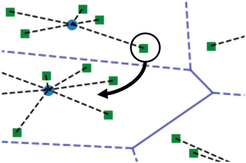
where $d_{i,k}$ is the distance between the location of customer $i$ and the cluster head $c_k$. After computing the distances of customers to their closest cluster heads, $D_1,D_2,\dots ,D_n$, we map customers $(1,2,\dots ,n)$ to $(b_1,b_2,\dots ,b_n)$ which belong to a priority queue $P=(b_1,b_2,\dots ,b_n)$ such that $D_{b_1}\le D_{b_2}\le \dots \le D_{b_n}$. This step is performed by the algorithmic routine in Alg.1.

Algorithm 1 Step 1 – algorithmic routine that returns the ordered list of customers, $P$

1: input: $\{d_{i,k}\},U{ }^{\mathrm{\prime }}$

2: for $i\in U{ }^{\mathrm{\prime }}$ do

3: compute $D_i$ by solving $\underset{k}{min}{d}_{i,k}$

4: set $P=(b_1,\dots ,b_n)$ such that $D_{b_1}\le \dots \le D_{b_n}$

5: output: $P=(b_1,\dots ,b_n)$

Step 2: In this step we assign customers to clusters. Starting from customer $b_1$ in the priority queue we perform the following:

We first initialize the set $C_{b_1}=K$ of the potential clusters where we can assign customer $b_1$ and we determine the closest cluster $k^{\ast }$ to customer $b_1$:

$k^{\ast }=\mathrm{a}\mathrm{r}\mathrm{g}\underset{k}{min}{d}_{b_1,k}$

Then, we check if:

• cluster $k^{\ast }$ has not reached its maximum allowed number of customers, $W$,

• the distance $d_{b_1,k^{\ast }}$ is smaller than or equal to the maximum allowed distance between a customer and a cluster head, $R$,

• and the accumulated customer demand in this cluster, ${\mu }_{b_1}+\sum _{j\in a_k^{\ast }}{\mu }_j$, where $\sum _{j\in a_k^{\ast }}{\mu }_j$ is the aggregate demand of all customers that are already in cluster $k^{\ast }$, is less than or equal to the vehicle capacity $Q$.

If all the above hold true, we add customer $b_1$ to the set of customers $a_k^{\ast }$ of cluster $k^{\ast }$. If not, customer $b_1$ is not assigned to cluster $k^{\ast }$ and we remove cluster $k^{\ast }$ from the set of the potential clusters for customer $b_1:C_{b_1}\leftarrow C_{b_1}\mathrm{\setminus }\{k^{\ast }\}$. Then, we perform the same checks for the remaining clusters in set $C_{b_1}$ until, hopefully, customer $b_1$ is assigned to a cluster.

If customer $b_1$ is assigned to a cluster $k$, we update the cluster head location of that cluster to represent the centroid (geometric center) of all customers in the cluster. The cluster head location for the extended set $a_k$ is calculated as

(10) $c_k=\frac{1}{|a_k|}\sum _{i\in a_k}{u}_i$(10)

where $|a_k|$ is the number of all customers in cluster $k$ that are stored in set $a_k$. This step terminates once we process all customers in the priority queue (see Alg.2).

Algorithm 2 Step 2 – algorithmic routine

1: input: $\{u_i\},W,R,\{{\mu }_i\},K,\{c_k\},\{d_{i,k}\},U$

2: execute Alg.1 to compute $P$

3: for $b_i\in P$ do

4: set $C_{b_i}=K$

5: while $b_i\in U\wedge C_{b_i}\ne \mathrm{\varnothing }$ do

6: set $k^{\ast }=\mathrm{a}\mathrm{r}\mathrm{g}\underset{k}{min}{d}_{b_i,k}$

7: if $|a_{k^{\ast }}|<W\wedge d_{b_i,k^{\ast }}\le R\wedge {\mu }_{b_1}+\sum _{j\in a_{k^{\ast }}}{\mu }_j\le Q$ then

8: $a_{k^{\ast }}\leftarrow a_{k^{\ast }}\cup \{b_i\}$

9: $c_k:=\frac{1}{|a_{k^{\ast }}|}\sum _{i\in a_{k^{\ast }}}{u}_i$

10: $U=U\mathrm{\setminus }\{b_i\}$

11: else

12: $C_{b_i}\leftarrow C_{b_i}\mathrm{\setminus }\{k^{\ast }\}$

13: output: $\{a_k\},\{c_k\}$

Step 3: In this step we remove all customers that are assigned to cluster sets $a_k$ and we keep only the updated locations of the cluster heads $c_k,\mathrm{\forall }k\in K$. With these updated cluster head locations, we perform again Steps 1 and 2 until the assignment of customers to clusters in two consecutive iterations of the algorithm does not change (convergence). If our algorithm has converged and not all customers are assigned to the $K$ clusters or there are clusters from the set $K$ with no customers, we incrementally increase or reduce, respectively, the number of clusters $|K|$ and we perform again all the steps of our clustering algorithm. This self-adaptation part of our clustering algorithm guarantees the assignment of all customers to clusters (Alg.3).

Algorithm 3 Constrained Clustering algorithm

1: while $a_k\ne \mathrm{\varnothing }\mathrm{\forall }k\in K\wedge U\ne \mathrm{\varnothing }$ do

2: $c_k\sim \mathcal{U}(u_1,\dots ,u_n),\mathrm{\forall }k\in K$, such that $c_k\ne c_j,\mathrm{\forall }j\in K$

3: $U\leftarrow \{1,\dots ,n\}$

4: $a_k\leftarrow \mathrm{\varnothing },\mathrm{\forall }k\in K$

5: while $(\{a_k{\}}_1^{|K|}{)}_{\mathrm{p}\mathrm{r}\mathrm{e}\mathrm{v}\mathrm{i}\mathrm{o}\mathrm{u}\mathrm{s}}\ne (\{a_k{\}}_1^{|K|})$ do

6: $(\{a_k{\}}_1^{|K|}{)}_{\mathrm{p}\mathrm{r}\mathrm{e}\mathrm{v}\mathrm{i}\mathrm{o}\mathrm{u}\mathrm{s}}\leftarrow (\{a_k{\}}_1^{|K|})$

7: $(\{a_k{\}}_1^{|K|})\leftarrow$ Alg.2

8: if $U\ne \mathrm{\varnothing }$ then

9: set $|K|\leftarrow |K|+1$, if there are unassigned customers

10: if $\mathrm{\exists }k|a_k=\mathrm{\varnothing }$ then

11: set $|K|\leftarrow |K|-1$ if there are clusters without customers: $a_k=\mathrm{\varnothing },$ for some $k\in K$

12: output: $\{c_k\},\{a_k\}$

Note that the assignment step of customers to clusters, the update step of the locations of the cluster heads, and the termination criterion are loosely based on the k-means algorithm. One main difference is that in our assignment step we do not always assign the customer to the closest cluster head because we require to satisfy also a number of distance and capacity-related constraints. In addition, our number of clusters $|K|$ can change if our algorithm fails to assign all customers to clusters.

Implementation Steps

To summarize, in Figure 4 we present the implementation steps of our constrained clustering approach for the capacitated vehicle routing problem (CC-CVRP).

Figure 4. Implementation overview of the CC-CVRP approach.

Initially, we use information regarding the network topology, the distances among customers and the number of available vehicles to implement the Constrained Clustering Algorithm (Alg.3). By doing so, we assign all our customers to clusters. Using the cluster head locations and the overall demand in each cluster, we solve the clustered CVRP presented in Equations (1)(1) $\underset{y_{kl}}{min}\sum _{k\in K}\sum _{l\in K}{d}_{kl}{y}_{kl}$(1) -(9(9) $y_{kk}=0,k\in K$(9) ) by using an external CVRP solver (i.e., one might use branch-and-cut or a heuristic solver). In this step we assign vehicles to clusters that include one or more customers. Finally, for each vehicle that needs to serve a number of customers from the clusters we solve a TSP to determine the optimal route of serving these customers.

Computational Complexity

Using the big O notation, the complexity of the original CVRP problem that considers actual customers instead of cluster heads is exponential. In particular, it is $O(2^{n^2})$ (Toth and Vigo 2002).

Solving a clustered CVRP reduces the number of decision variables by a factor of $r=n/|K|$, hence the complexity of the clustered CVRP is reduced to $O(2^{{(n/r)}^2})$. Once the clustering problem is solved, we still have to solve singular TSP problems for every vehicle that is assigned to one or more clusters. The complexity of each TSP problem depends on the number of customers visited by the respective vehicle. When using the well-known Held-Karp algorithm, the worst-case complexity of the TSP is $O(m^2{2}^m)$, where $m$ is the number of visited customers. If we have $V$ assigned vehicles, the number of customers served by each vehicle is $m\approx n/V$, and the complexity of this step is $O((n/V{)}^2{2}^{(n/V)})$. Because we need to solve the TSP for all vehicles $V$, the worst-case complexity of our CC-CVRP approach is $O((n^2/V)2^{(n/V)}+O(2^{n^2/r^2})$. If $|K|<n$, the computational complexity $O(2^{n^2/r^2})$ dominates complexity $O((n^2/V)2^{(n/V)}$ in large problem instances resulting in a worst-case complexity of $O(2^{n^2/r^2})$.

To summarize, by solving a clustered CVRP instead of the original CVRP we reduce the worst-case time complexity from $O(2^{n^2})$ to $O(2^{n^2/r^2})$. In the extreme case that the number of clusters is equal to the number of customers, $|K|=n$, then $r=1$ and the complexity of the proposed approach becomes $O((n^2/V)2^{(n/V)}+O(2^{n^2})$. As expected, the proposed approach does not offer a benefit in terms of computational complexity in the extreme case where one assigns a cluster to each customer. If, however, we assign several customers to a cluster our method results in a time complexity reduction from $O(2^{n^2})$ to $O(2^{n^2/r^2})$.

Numerical Experiments

Assessment Framework and Benchmark Datasets

Our CC-CVRP maps the original CVPR problem into a reduced dimension problem (see Alg.3). While the time complexity gain when using the proposed approach is exponential, the searched solution space is reduced, potentially excluding the optimal solution. We evaluate both the computational costs and the optimality gaps using a large number of publicly available problem instances designed for benchmarking solution approaches for the CVRP. We evaluate the quality gap, defined as the relative performance difference between:

(a) the solution of our CC-CVRP approach,

(b) and the proven optimal or best known solution reported in http://vrp.galgos.inf.puc-rio.br for the respective problem instances.

We note that to solve the clustered CVRP problem in Equations (1)(1) $\underset{y_{kl}}{min}\sum _{k\in K}\sum _{l\in K}{d}_{kl}{y}_{kl}$(1) -(9(9) $y_{kk}=0,k\in K$(9) ) we need to use branch-and-cut to compute a globally optimal solution or a heuristic to compute an approximate solution. In addition, we need to solve subsequent TSP problems for each single vehicle and this might result in higher computation costs in some problem instances, as discussed in our previous section. This is investigated in our numerical experiments where we test the computation costs and the solution quality of the proposed approach.

In our implementation, the TSP problems are solved using the tspy Python package that implements the TwoOpt local search algorithm. All tests are conducted in a general-purpose computer with a 2.3 GHz Intel Core 5 processor and a 16GB RAM. Our test instances include the following instances that are publicly available at http://vrp.galgos.inf.puc-rio.br:

• Small-scale instances A with 32 to 82 customers.

• Medium-scale instances X with 101 to 350 customers.

• Large-scale instances X with 350 to 1001 customers.

• Very large-scale instances with 3000 to 16000 customers.

Small-scale Instances

As previously mentioned, globally optimal solutions for the NP-Hard CVRP problem can be computed only in small-scale instances. For this, we initially use as benchmark small problem instances that belong to class A described in Uchoa et al. (2017). These test instances and their globally optimal solutions are publicly available at http://vrp.galgos.inf.puc-rio.br.

In this initial investigation, we report the performance when solving our CC-CVPR and the original CVRP when imposing a time limit of 100 seconds. Then, we compare the solution of our CC-CVPR and the solution of the original CVRP against the globally optimal solution available at http://vrp.galgos.inf.puc-rio.br. Our objective is twofold: first, to investigate the optimality gap of our CC-CVRP solution with respect to the globally optimal solution; second, to investigate the performance improvement of our CC-CVRP solution compared to the solution of the original CVRP problem when using a time limit of 100 seconds for both methods. The latter will show us whether clustering can lead to better solutions by allowing to explore the solution space more efficiently.

As discussed, to ensure an unbiased comparison we use the same computation budget of 100 seconds when solving the CC-CVRP and the original CVRP. The results from all small-scale problem instances in class A are reported in Table 2 where we present the optimality gap(s) when solving the CC-CVRP and the original CVRP with respect to the globally optimal solution. In more detail, column 1 presents the identification number of the problem instance that belongs to the A class. Each instance is coded as A-nXX-kY where XX refers to the number of customers including the depot, and Y to the number of vehicles. Column 2 presents the tightness of the instance, which is the equal to the total demand divided by the vehicle capacity. Column 3 presents the dispersion of the instance, which is the standard deviation of the histogram of the distances over the mean. Column 4 presents the best-known solution reported in http://vrp.galgos.inf.puc-rio.br and column 5 states whether this solution is a proven optimal. We note that all solutions of the instances of class A reported in column 4 are globally optimal. Column 6 presents the performance of the CC-CVRP solution and column 7 presents the optimality gap of this solution with respect to the globally optimal solution presented in column 4. Finally, columns 8 and 9 present the performance and the optimality gap of the solution when solving the original CVRP problem without considering clusters. Note that the CC-CVRP and original CVRP solutions are the best found solutions within 100 seconds.

Table 2. Performance evaluation for the class A instances of Augerat et al. (1995) reported in http://vrp.galgos.inf.puc-rio.br

instance	tightness	dispersion	best known	proven	CC-CVRP		CVRP
			solution	optimal
					solution	optimality	solution	optimality
						gap (%)		gap (%)
A-n32-k5	4.1	49.40	784	yes	832	6.1	797	1.7
A-n33-k5	4.5	54.10	661	yes	691	4.6	776	17.4
A-n33-k6	5.4	53.40	742	yes	812	9.4	812	9.4
A-n34-k5	4.6	52.27	778	yes	796	2.3	857	10.2
A-n36-k5	4.4	51.29	799	yes	849	6.3	870	8.9
A-n37-k5	4.1	49.33	669	yes	717	7.2	673	0.7
A-n37-k6	5.7	48.83	949	yes	1061	11.8	1025	8
A-n38-k5	4.8	50.19	730	yes	827	13.3	837	14.6
A-n39-k5	4.8	50.57	822	yes	895	8.9	846	2.9
A-n39-k6	5.3	48.42	831	yes	907	9.2	902	8.6
A-n44-k6	5.7	50.97	937	yes	1034	10.4	1032	10.1
A-n45-k7	6.3	48.77	1146	yes	1208	5.4	1167	1.8
A-n46-k7	6.0	50.10	914	yes	1029	12.5	1057	15.7
A-n48-k7	6.3	50.17	1073	yes	1158	7.9	1168	8.9
A-n53-k7	6.6	49.31	1010	yes	1204	19.2	1119	10.8
A-n54-k7	6.7	48.82	1167	yes	1254	7.5	1288	10.4
A-n55-k9	8.4	49.42	1073	yes	1205	12.3	1174	9.4
A-n60-k9	8.3	48.45	1354	yes	1504	11.1	1523	12.5
A-n61-k9	8.9	49.12	1034	yes	1301	25.8	1720	66.3
A-n62-k8	7.3	49.16	1288	yes	1402	8.9	1414	9.8
A-n63-k9	9.3	49.38	1616	yes	1827	13	1827	13.1
A-n63-k10	9.3	49.47	1314	yes	1420	8.1	1436	9.3
A-n64-k9	8.5	49.04	1401	yes	1545	10.3	1515	8.1
A-n65-k9	8.8	47.26	1174	yes	1358	15.7	1284	9.4
A-n69-k9	8.5	48.64	1159	yes	1241	7.1	1231	6.2
A-n80-k10	9.4	49.63	1763	yes	1910	8.3	1959	11.1
Average						10.1		11.4

From Table 2 one can note that the CC-CVRP solutions have an average optimality gap of 10.1% with a standard deviation of 4.8% when compared against the respective globally optimal solutions. In contrast, the average optimality gap of the solutions of the original CVRP problem is 11.4% (1.3% higher). This demonstrates that the proposed approach used more efficiently the 100-second computation budget to find improved solutions.

We further compare the results of our approach against the results of Shalaby, Mohammed, and Kassem (2021) who developed a Cluster-First Route-Second Method (CFRS) approach where customers are first divided into clusters, and then each cluster is solved independently as a TSP. Shalaby, Mohammed, and Kassem (2021) used a Fuzzy C-Means (FCM) clustering technique to assign customers into clusters. In their work, they present results for instances A-n32-k5, A-n33-k6, A-n36-k5, A-n33-k5, and A-n39-k6 after running their algorithm for up to 15 minutes. Their results are presented in the 4th column of Table 3. When comparing their results against the results of CC-CVRP, the CC-CVRP solution performs better in instances A-n32-k5, A-n36-k5 and A-n33-k5, whereas the FCM solution performs better in instances A-n33-k6 and A-n39-k6. We should note, however, that the FCM has a computation budget of 15 minutes, whereas the proposed CC-CVRP approach has a computation budget of only 100 seconds.

Table 3. Comparison of CC-CVRP solutions computed in up to 100 seconds and the FCM solutions of Shalaby, Mohammed, and Kassem (2021) computed in up to 15 minutes

instance	best known solution	CC-CVRP	Original FCM
A-n32-k5	784	832	840
A-n33-k6	742	812	769
A-n36-k5	799	849	857
A-n33-k5	661	691	695
A-n39-k6	831	895	876

In the following sections of our numerical experiments we present the performances of the CC-CVRP solutions and their optimality gaps with respect to best-known solutions for medium-scale, large-scale, and very large-scale problem instances. Note that we do not provide results regarding the solutions of the original CVRP for these larger instances because it is not possible to find such solutions within 100 seconds due to the computational complexity of the original CVRP.

Medium-scale Instances

In the medium-scale instances we present the results when solving our CC-CVRP within 100 seconds for the X instances with up to 350 customers (see Table 4). The best-known solutions of these instances are publicly available at http://vrp.galgos.inf.puc-rio.br and in column 5 we declare which ones of them are globally optimal and which are just best-known. On average, the optimality gap of our CC-CVRP solutions is 9% with a standard deviation of 4.4%.

Table 4. Performance evaluation for the instances of class X for $100<n<350$ reported in http://vrp.galgos.inf.puc-rio.br

instance	tightness	dispersion	best known solution	proven optimal	CC-CVRP
					solution	optimality
						gap (%)
X-n101-k25	25.0	51.12	27591	yes	29838	8.1
X-n106-k14	13.1	64.67	26362	yes	27515	4.4
X-n110-k13	12.4	48.75	14971	yes	16885	12.8
X-n120-k6	5.7	49.46	13332	yes	14279	7.1
X-n125-k30	29.4	60.09	55539	yes	58535	5.4
X-n129-k18	17.1	49.51	28940	yes	32101	10.9
X-n134-k13	12.8	63.15	10916	yes	12319	12.9
X-n139-k10	9.8	47.99	13590	yes	15973	17.5
X-n148-k46	45.4	51.51	43448	yes	45358	4.4
X-n157-k13	13.0	71.20	16876	yes	17751	5.2
X-n162-k11	10.4	51.06	14138	yes	15354	8.6
X-n167-k10	9.3	48.70	20557	yes	22891	11.4
X-n172-k51	50.3	50.54	45607	yes	48406	6.1
X-n181-k23	22.5	58.34	25569	yes	26315	2.9
X-n186-k15	14.2	48.60	24145	yes	27121	12.3
X-n190-k8	7.6	74.32	16980	yes	18168	7
X-n195-k51	50.9	50.42	44225	yes	48409	9.5
X-n200-k36	35.5	70.58	58578	yes	60922	4
X-n204-k19	18.1	54.57	19565	yes	22157	13.2
X-n209-k16	15.3	48.84	30656	yes	33128	8.1
X-n214-k11	11.0	53.94	10856	yes	13163	21.2
X-n219-k73	72.7	48.18	117595	yes	118305	0.6
X-n223-k34	33.4	50.52	40437	yes	44187	9.3
X-n228-k23	16.0	51.70	25742	yes	28649	11.3
X-n233-k16	13.1	48.45	19230	yes	21346	11
X-n237-k14	47.3	48.66	27042	yes	29594	9.4
X-n242-k48	27.1	55.36	82751	yes	87106	5.3
X-n251-k28	27.1	55.18	38684	yes	40661	5.1
X-n256-k16	15.9	51.41	18839	no	20623	9.5
X-n261-k13	12.4	48.77	26558	yes	30318	14.2
X-n266-k58	57.6	52.36	75478	yes	78460	4
X-n270-k35	34.9	51.57	35291	yes	37116	5.2
X-n275-k28	27.4	54.18	21245	yes	22666	6.7
X-n280-k17	16.8	48.72	33503	no	37602	12.2
X-n284-k15	14.0	54.38	20215	yes	22953	13.5
X-n289-k60	59.8	50.84	95151	yes	100104	5.2
X-n294-k50	49.6	48.34	47161	no	51941	10.1
X-n298-k31	30.7	48.26	34231	yes	39052	14.1
X-n303-k21	20.1	59.65	21736	no	24867	14.4
X-n308-k13	12.7	49.47	25859	no	29168	12.8
X-n313-k71	70.7	54.00	94043	no	101650	8.1
X-n317-k53	52.7	62.73	78355	yes	79023	0.9
X-n322-k28	27.7	48.55	29834	yes	34597	16
X-n327-k20	19.2	51.13	27532	no	30735	11.6
X-n331-k15	14.3	48.50	31102	yes	33929	9.1
X-n336-k84	83.4	48.65	139111	no	145695	4.7
X-n344-k43	42.7	50.11	42050	no	45300	7.7
Average						9.0

Large-scale Instances

In the large-scale instances we present the results when solving our CC-CVRP within 100 seconds for the X instances with customers ranging from 350 to 1001 (see Table 5). The best-known solutions of these instances are publicly available at http://vrp.galgos.inf.puc-rio.br and in column 5 we declare which ones of them are globally optimal and which are just best-known. On average, the optimality gap of our CC-CVRP solutions is 8.7% with a standard deviation of 4%.

Table 5. Performance evaluation for the instances of class X for $n\ge 350$ reported in http://vrp.galgos.inf.puc-rio.br

instance	tightness	dispersion	best known solution	proven optimal	CC-CVRP
					solution	optimality
						gap (%)
X-n351-k40	39.7	60.14	25896.0	no	28745	11
X-n359-k29	28.6	49.46	51505.0	no	55485	7.7
X-n367-k17	16.7	54.53	22814.0	no	25236	10.6
X-n376-k94	93.8	48.60	147713.0	yes	148790	0.7
X-n384-k52	51.7	48.24	65938.0	no	69757	5.8
X-n393-k38	37.4	56.76	38260.0	yes	41846	9.4
X-n401-k29	28.6	56.13	66154	no	69155	4.5
X-n411-k19	18.1	59.59	19712	no	22694	15.1
X-n420-k130	129.2	55.35	107798	yes	113708	5.5
X-n429-k61	60.2	47.99	65449	no	70343	7.5
X-n439-k37	36.5	50.03	36391	yes	39359	8.2
X-n449-k29	28.9	48.46	55233	no	60931	10.3
X-n459-k26	25.7	60.44	24139	no	27636	14.5
X-n491-k59	58.3	51.61	66483	no	71898	8.1
X-n502-k39	38.5	72.96	69226	no	70986	2.5
X-n513-k21	20.5	53.94	24201	no	28422	17.4
X-n548-k50	49.7	48.19	86700	yes	91028	5
X-n561-k42	41.3	49.38	42717	no	48334	13.1
X-n573-k30	29.4	60.66	50673	no	54030	6.6
X-n586-k159	158.2	51.65	190316	no	200107	5.1
X-n599-k92	91.9	48.19	108451	no	113937	5.1
X-n613-k62	61.2	48.22	59535	no	67638	13.6
X-n627-k43	42.8	64.79	62164	no	66463	6.9
X-n641-k35	34.4	50.68	63684	no	69888	9.7
X-n655-k131	130.8	63.67	106780	yes	107824	1
X-n685-k75	74.3	50.41	68205	no	79762	16.9
X-n701-k44	43.6	51.09	81923	no	89991	9.8
X-n716-k35	34.0	63.87	43373	no	47091	8.6
X-n733-k159	158.8	48.19	136187	no	147320	8.2
X-n749-k98	97.0	51.86	77269	no	83399	7.9
X-n766-k71	70.5	50.80	114417	no	127806	11.7
X-n783-k48	47.4	48.00	72386	no	80590	11.3
X-n801-k40	40.0	48.29	73305	no	79500	8.5
X-n876-k59	58.3	66.01	99299	no	105036	5.8
X-n895-k37	36.9	48.17	53860	no	60440	12.2
X-n957-k87	86.9	52.81	85465	no	90644	6.1
X-n979-k58	57.5	66.58	118976	no	125254	5.3
X-n1001-k43	42.4	48.04	72355	no	82174	13.6
Average						8.7

Very Large-scale Instances

In the very large-scale instances we present the results when solving our CC-CVRP within 100 seconds for the instances of Arnold, Gendreau, and Kenneth (2019a) with customers ranging from 3000 to 16000 (see Table 6). The best-known solutions of these instances are publicly available at http://vrp.galgos.inf.puc-rio.br. On average, the optimality gap of our CC-CVRP solutions is 15.7% with a standard deviation of 5.3%.

Table 6. Performance evaluation for the instances of Arnold, Gendreau, and Kenneth (2019a) presented in http://vrp.galgos.inf.puc-rio.br

instance	best known solution	proven optimal	CC-CVRP
			solution	optimality
				gap (%)
Antwerp1-n6000	477277	no	535304	12.2
Antwerp2-n7000	291371	no	332856	14.2
Brussels2-n16000	345551	no	432440	25.1
Ghent2-n11000	257802	no	301728	17.0
Leuven1-n3000	192848	no	211946	9.9
Leuven2-n4000	111399	no	128756	15.6
Average				15.7

Conclusion

This study introduced an approach for solving very large-scale instances of the Capacitated Vehicle Routing Problem (CVRP) based on the use of a constrained clustering algorithm that clusters customers and solves a CVRP considering the cluster heads. At its first stage, the proposed approach assigns vehicles to clusters. This is achieved by introducing a self-adapting clustering algorithm that is loosely based on k-means. At its second stage, we determine the tour of each vehicle by solving a TSP considering the set of customers that belong to the assigned clusters of that vehicle.

Our proposed CC-CVRP approach is applied in a large number of benchmark scenarios described in Uchoa et al. (2017) and available at http://vrp.galgos.inf.puc-rio.br considering three different solvers. Our experiments demonstrate that our CC-CVRP approach returns solutions that outperform the solutions of solving the unclustered CVRP in small-sized problem instances by 1.3% in terms of solution quality. For larger problem instances, it is not even possible to compute solutions when solving the unclustered (original) CVRP within a computational budget of 100 seconds. Our CC-CVRP approach, however, was capable of finding improved solutions even for very large problem instances with up to 16000 customers. In particular, it exhibited:

• an average optimality gap of 10.1% and a standard deviation of 4.8% in small-sized instances;

• an average optimality gap of 9% and a standard deviation of 4.4% in medium-sized instances;

• an average optimality gap of 8.9% and a standard deviation of 4% in large-sized instances;

• an average optimality gap of 15.7% and a standard deviation of 5.3% in very large-sized instances.

In future research, one can expand further our method to apply it in different types of VRP, such as the Vehicle Routing Problem with Time Windows (VRPTW) and the Vehicle Routing Problem with Profits (VRPP). The proposed approach can also be extended by considering the development of multiple clusters with the use of different hyper-parameters (e.g., number of customers per cluster) and selecting the best setting. In addition, learning-based methods, such as neural network clustering, can be used to offer adaptive clustering by learning the characteristics of specific types of problem instances.

Disclosure statement

No potential conflict of interest was reported by the author(s).

References

- Archetti, C., E. Fernandez, and D. L. Huerta-Muñoz. 2017. The flexible periodic vehicle routing problem. Computers & Operations Research 85:201–225. doi:10.1016/j.cor.2017.03.008.
- Archetti, C., L. Bertazzi, G. Laporte, and M. Grazia Speranza. 2007. A branch-and-cut algorithm for a vendor-managed inventory-routing problem. Transportation Science 41 (3):382–91. doi:10.1287/trsc.1060.0188.
- Archetti, C., M. Christiansen, and M. Grazia Speranza. 2018. Inventory routing with pickups and deliveries. European Journal of Operational Research 268 (1):314–24. https://www.sciencedirect.com/science/article/pii/S0377221718300109.
- Archetti, C., and M. Grazia Speranza. 2013. Vehicle routing problems with split deliveries. International Transactions in Operational Research 19:3–22. doi:10.1111/j.1475-3995.2011.00811.x.
- Archetti, C., and M. Grazia Speranza. 2016. The inventory routing problem: The value of integration. International Transactions in Operational Research 23:393–407. doi:10.1111/itor.12226.
- Archetti, C., M. W. P. Savelsbergh, and M. Grazia Speranza. 2006. Worst-case analysis for split delivery vehicle routing problems. Transportation Science 40:226–34. doi:10.1287/trsc.1050.0117.
- Archetti, C., N. Bianchessi, S. Irnich, and M. Grazia Speranza. 2014. Formulations for an inventory routing problem. International Transactions in Operational Research 21:353–74. doi:10.1111/itor.12076.
- Archetti, C., O. Jabali, and M. Grazia Speranza. 2015. Multi-period vehicle routing problem with due dates. Computers & Operations Research 61:122–34. https://www.sciencedirect.com/science/article/pii/S0305054815000726.
- Arnold, F., M. Gendreau, and S. Kenneth. 2019a. Efficiently solving very large-scale routing problems. Computers& Operations Research 107:32–42. doi:10.1016/j.cor.2019.03.006.
- Augerat, P., D. Naddef, J. M. Belenguer, E. Benavent, A. Corberan, and G. Rinaldi. 1995. “Computational results with a branch and cut code for the capacitated vehicle routing problem.”.
- Baldacci, R., N. Christofides, and A. Mingozzi. 2008. An exact algorithm for the vehicle routing problem based on the set partitioning formulation with additional cuts. Mathematical Programming 115 (2):351–85. doi:10.1007/s10107-007-0178-5.
- Bertazzi, L., M. Savelsbergh, and M. Grazia Speranza. 2008. Inventory routing, 49–72. Boston, MA: Springer US. doi:10.1007/978-0-387-77778-8_3.
- Bodin, L. 1983. Routing and scheduling of vehicles and crews, the state of the art. Computers & Operations Research 10 (2):63–211.
- Braekers, K., K. Ramaekers, and I. Van Nieuwenhuyse. 2016. The vehicle routing problem: State of the art classification and review. Computers & Industrial Engineering 99:300–13. https://www.sciencedirect.com/science/article/pii/S0360835215004775.
- Bujel, K., F. Lei, M. Szczecinski, S. Winnie, and M. Fernandez. 2019. “Solving high volume capacitated vehicle routing problem with time windows using recursive-DBSCAN clustering algorithm.” arXiv:1812.02300v2 [cs.OH] Accessed 2019-March-23. http://arxiv.org/abs/1812.02300.
- Campbell, A. M., and J. H. Wilson. 2014. Forty years of periodic vehicle routing. Networks 63 (1):2–15. doi:10.1002/net.21527.
- Campbell, A. M., and J. R. Hardin. 2005. Vehicle minimization for periodic deliveries. European Journal of Operational Research 165 (3):668–84. https://www.sciencedirect.com/science/article/pii/S0377221704001262.
- Christofides, N. 1985. “Vehicle routing in the traveling salesman problem-In a guided tour of combinatorial optimization, 431-448.” Great Britain.: John Wiley & Sons Ltd.
- Christofides, N., A. Mingozzi, and P. Toth. 1981a. Exact algorithms for the vehicle routing problem, based on spanning tree and shortest path relaxations. Mathematical Programming 20 (1):255–82. doi:10.1007/BF01589353.
- Christofides, N., A. Mingozzi, and P. Toth. 1981b. “State-space relaxation procedures for the computation of bounds to routing problems.” Networks 11 (2):145–64. doi:10.1002/net.3230110207.
- Clarke, G., and J. W. Wright. 1964. Scheduling of vehicles from a central depot to a number of delivery points. Operations Research 12 (4):568–81. doi:10.1287/opre.12.4.568.
- Coelho, L. C., J.-F. Cordeau, and G. Laporte. 2014. Thirty years of inventory routing. Transportation Science 48 (1):1–158. doi:10.1287/trsc.2013.0472.
- Dantzig, G. B., and J. H. Ramser. 1959. The truck dispatching problem. Management Science 6 (1):80–91. doi:10.1287/mnsc.6.1.80.
- Defryn, C., and S. Kenneth. 2017. A fast two-level variable neighborhood search for the clustered vehicle routing problem. Computers & Operations Research 83:78–94. doi:10.1016/j.cor.2017.02.007.
- Dorronsoro, B., D. Arias, F. Luna, A. J. Nebro, and E. Alba. 2007. “A grid-based hybrid cellular genetic algorithm for very large scale instances of the CVRP.” In 2007 High Performance Computing & Simulation Conference (HPCS 2007), 759–65.
- Eilon, S., C. D. T. Watson-Gandy, N. Christofides, and R. de Neufville. 1974. Distribution management-mathematical modelling and practical analysis. IEEE Transactions on Systems, Man, and Cybernetics SMC-4 (6):589–589. doi:10.1109/TSMC.1974.4309370.
- Faiz, S., S. Krichen, and W. Inoubli. 2014. A DSS based on GIS and Tabu search for solving the CVRP: The Tunisian case. The Egyptian Journal of Remote Sensing and Space Science 17 (1):105–10. doi:10.1016/j.ejrs.2013.10.001.
- Fisher, M. L., and R. Jaikumar. 1978. A decomposition algorithm for large-scale vehicle routing. Department of Decision Sciences, Wharton School, University of Pennsylvania.
- Fisher, M. 1995. Vehicle routing. Handbooks in Operations Research and Management Science 8:1–33.
- Forgy, E. W. 1965. Cluster analysis of multivariate data: Efficiency versus interpretability of classifications. biometrics 21:768–69.
- Gadegaard, S. L., and J. Lysgaard. 2021. A symmetry-free polynomial formulation of the capacitated vehicle routing problem. Discrete Applied Mathematics 296:179–92. doi:10.1016/j.dam.2020.02.012.
- Gendreau, M., A. Hertz, and G. Laporte. 1994. A tabu search heuristic for the vehicle routing problem. Management Science 40 (10):1276–90. doi:10.1287/mnsc.40.10.1276.
- Gendreau, M., J.-Y. Potvin, O. Bräumlaysy, G. Hasle, and L. Arne. 2008b. Metaheuristics for the vehicle routing problem and its extensions: A categorized bibliography, 143–69. Boston, MA: Springer US. doi:10.1007/978-0-387-77778-8_7.
- Gendreau, M., M. Iori, G. Laporte, and S. Martello. 2008a. A Tabu search heuristic for the vehicle routing problem with two-dimensional loading constraints. Networks: An International Journal 51 (1):4–18. doi:10.1002/net.20192.
- Gillett, B. E., and L. R. Miller. 1974. A heuristic algorithm for the vehicle-dispatch problem. Operations Research 22 (2):340–49. doi:10.1287/opre.22.2.340.
- Golden, B. L., S. Raghavan, and E. A. Wasil. 2008. The vehicle routing problem: Latest advances and new challenges, vol. 43. Springer Science & Business Media.
- Gulczynski, D., B. Golden, and E. Wasil. 2011. The period vehicle routing problem: New heuristics and real-world variants. Transportation Research Part E: Logistics and Transportation Review 47 (5):648–68. https://www.sciencedirect.com/science/article/pii/S1366554511000196.
- Hintsch, T., and S. Irnich. 2020. Exact solution of the soft-clustered vehicle-routing problem. European Journal of Operational Research 280 (1):164–78. doi:10.1016/j.ejor.2019.07.019.
- Huang, M., and H. Xiangpei. 2012. Large scale vehicle routing problem: An overview of algorithms and an intelligent procedure. International Journal of Innovative Computing, Information and Control 8 (8):5809–19.
- Konstantakopoulos, G. D., S. P. Gayialis, and E. P. Kechagias. 2020. Vehicle routing problem and related algorithms for logistics distribution: A literature review and classification. In Operational research, 1–30.
- Laporte, G., and Y. Nobert. 1987. Exact algorithms for the vehicle routing problem. In North-Holland mathematics studies, vol. 132, 147–84. Elsevier.
- Laporte, G. 1992. The vehicle routing problem: An overview of exact and approximate algorithms. European Journal of Operational Research 59 (3):345–58. doi:10.1016/0377-2217(92)90192-C.
- Laporte, G. 2009. Fifty years of vehicle routing. Transportation Science 43 (4):408–16. doi:10.1287/trsc.1090.0301.
- Lau, H. C., Q. Liu, and H. Ono. 2002. “Integrating local search and network flow to solve the inventory routing problem.” In Eighteenth National Conference on Artificial Intelligence, Vol. 2, USA, 9–14. American Association for Artificial Intelligence.
- Lee, C.-Y., Z.-J. Lee, S.-W. Lin, and K.-C. Ying. 2010. An enhanced ant colony optimization (EACO) applied to capacitated vehicle routing problem. Applied Intelligence 32 (1):88–95. doi:10.1007/s10489-008-0136-9.
- Leung, S. C. H., J. Zheng, D. Zhang, and X. Zhou. 2010. Simulated annealing for the vehicle routing problem with two-dimensional loading constraints. Flexible Services and Manufacturing Journal 22 (1–2):61–82. doi:10.1007/s10696-010-9061-4.
- Li, F., B. Golden, and E. Wasil. 2005. Very large-scale vehicle routing: New test problems, algorithms, and results. Computers & Operations Research 32:1165–79. doi:10.1016/j.cor.2003.10.002.
- Li, F., B. Golden, and E. Wasil. 2007. The open vehicle routing problem: Algorithms, large-scale test problems, and computational results. International Journal of Applied Engineering Research 34 (10):2918–30.
- Lloyd, S. 1982. Least squares quantization in PCM. IEEE Transactions on Information Theory 28 (2):129–37. doi:10.1109/TIT.1982.1056489.
- Magnanti, T. L. 1981. Combinatorial optimization and vehicle fleet planning: Perspectives and prospects. Networks 11 (2):179–213. doi:10.1002/net.3230110209.
- Mazzeo, S., and I. Loiseau. 2004. An ant colony algorithm for the capacitated vehicle routing. Electronic Notes in Discrete Mathematics 18:181–86. doi:10.1016/j.endm.2004.06.029.
- Miller, C. E., A. W. Tucker, and R. A. Zemlin. 1960. Integer programming formulation of traveling salesman problems. Journal of the ACM (JACM) 7 (4):326–29. doi:10.1145/321043.321046.
- Mor, A., and M. Grazia Speranza. 2020. Vehicle routing problems over time: A survey. 4OR-Q J Oper Res 18:129–49. doi:10.1007/s10288-020-00433-2.
- Mostafa, N., and A. Eltawil. 2017. “Solving the heterogeneous capacitated vehicle routing problem using K-means clustering and valid inequalities.” In Proceedings of the International Conference on Industrial Engineering and Operations Management.
- Naddef, D., and G. Rinaldi. 2002. Branch-and-cut algorithms for the capacitated VRP. In The vehicle routing problem, 53–84. SIAM.
- Nazif, H., and L. S. Lee. 2012. Optimised crossover genetic algorithm for capacitated vehicle routing problem. Applied Mathematical Modelling 36 (5):2110–17. doi:10.1016/j.apm.2011.08.010.
- Pecin, D., A. Pessoa, M. Poggi, and E. Uchoa. 2017. Improved branch-cut-and-price for capacitated vehicle routing. Mathematical Programming Computation 9 (1):61–100. doi:10.1007/s12532-016-0108-8.
- Petrakis, I., C. Hass, and M. Bichler. 2012. On the impact of real-time information on field service scheduling. Decision Support Systems 53 (2):282–93. doi:10.1016/j.dss.2012.01.013.
- Qu, Z. W., L. N. Cai, C. Li, and L. Zheng. 2004. Solution framework for the large scale vehicle deliver/collection problem. Journal of Tsinghua University (Sci. & Tech.) 44 (5):581–84.
- Savelsbergh, M., and J.-H. Song. 2007. Inventory routing with continuous moves. Computers & Operations Research 34 (6):1744–63. Part Special Issue: Odysseus 2003 Second International Workshop on Freight Transportation Logistics. doi:10.1016/j.cor.2005.05.036.
- Shalaby, M., A. Mohammed, and S. Kassem. 2021. Supervised Fuzzy C-means techniques to solve the capacitated vehicle routing problem. INTERNATIONAL ARAB JOURNAL OF INFORMATION TECHNOLOGY 18 (3 A):452–63.
- Singanamala, P. K., D. Reddy, and P. Venkataramaiah. 2018. Solution to a multi depot vehicle routing problem using K-means Algorithm, Clarke and Wright algorithm and Ant Colony optimization. International Journal of Applied Engineering Research 13 (21):15236–46.
- Song, B. D., K. Park, and J. Kim. 2018. Persistent UAV delivery logistics: MILP formulation and efficient heuristic. Computers & Industrial Engineering 120:418–28. doi:10.1016/j.cie.2018.05.013.
- Syrichas, A., and A. J. Crispin. 2017. Large-scale vehicle routing problems: Quantum annealing, tunings and results. Computers & Operations Research 87:52–62. doi:10.1016/j.cor.2017.05.014.
- Tasan, A. S., and M. Gen. 2012. A genetic algorithm based approach to vehicle routing problem with simultaneous pick-up and deliveries. Computers & Industrial Engineering 62 (3):755–61. doi:10.1016/j.cie.2011.11.025.
- Tavakkoli-Moghaddam, R., N. Safaei, and Y. Gholipour. 2006. A hybrid simulated annealing for capacitated vehicle routing problems with the independent route length. Applied Mathematics and Computation 176 (2):445–54. doi:10.1016/j.amc.2005.09.040.
- Toth, P., and D. Vigo. 2002. Models, relaxations and exact approaches for the capacitated vehicle routing problem. Discrete Applied Mathematics 123 (1–3):487–512. doi:10.1016/S0166-218X(01)00351-1.
- Toth, P., and D. Vigo. 2003. The granular tabu search and its application to the vehicle-routing problem. Informs Journal on Computing 15 (4):333–46. doi:10.1287/ijoc.15.4.333.24890.
- Toth, P., and D. Vigo. 2014. Vehicle routing: Problems, methods, and applications. SIAM.
- Tu, W., L. Qingquan, L. Qiuping, J. Zhu, B. Zhou, and B. Y. Chen. 2017. A spatial parallel heuristic approach for solving very large-scale vehicle routing problems. Transactions in GIS 21 (3):1–18. doi:10.1111/tgis.12267.
- Uchoa, E., D. Pecin, A. Pessoa, M. Poggi, T. Vidal, and A. Subramanian. 2017. New benchmark instances for the capacitated vehicle routing problem. European Journal of Operational Research 257 (3):845–58. doi:10.1016/j.ejor.2016.08.012.
- Wang, K., Y. Shao, and W. Zhou. 2017. Matheuristic for a two-echelon capacitated vehicle routing problem with environmental considerations in city logistics service. Transportation Research Part D: Transport and Environment 57:262–76. doi:10.1016/j.trd.2017.09.018.
- Wren, A., and A. Holliday. 1972. Computer scheduling of vehicles from one or more depots to a number of delivery points. Journal of the Operational Research Society 23 (3):333–44. doi:10.1057/jors.1972.53.
- Zhang, Y., Y. Mei, K. Tang, and K. Jiang. 2017. Memetic algorithm with route decomposing for periodic capacitated arc routing problem. Applied Soft Computing 52:1130–42. doi:10.1016/j.asoc.2016.09.017.
- Zhu, W., H. Qin, A. Lim, and L. Wang. 2012. A two-stage tabu search algorithm with enhanced packing heuristics for the 3L-CVRP and M3L-CVRP. Computers & Operations Research 39 (9):2178–95. doi:10.1016/j.cor.2011.11.001.