Predicting the Contribution of Mining Sector to the Gross Domestic Product (GDP) Index Utilizing Heuristic Approaches

ABSTRACT

GDP is a measure of the size of the economy and how an economy is performing. The mining industry has become a focal point in the total economic picture of many countries; however, the factors affecting the contribution of the mining sector to the growth of GDP (GDP_MS) have not been investigated in depth yet. In this paper, heuristic approaches were adopted to predict the GDP_MS. Therefore, the effect of three parameters, namely, value added of GDP, the value of industrial output per capita and per capita value added on GDP _MS, has been investigated. For this purpose, the data of countries that are actively participating in the mining industry was applied to a hybrid intelligent technique and an effective model was proposed. The results showed that a combination of a neuro-fuzzy inference system and a genetic algorithm has relatively the best performance to predict GDP_MS. Furthermore, multiple parametric sensitivity analysis was conducted on the output of the model, and the outcomes showed that GDP_MS is highly sensitive to all three input parameters; also, per capita value added and value added of GDP have the highest and the least effect on GDP_MS, respectively.

Introduction

Macroeconomics is a branch of economics that is linked to macroeconomic efficiency, structure, behavior, and economic decision-making. The macroeconomic field includes a national, regional, and global economy (Clements et al. 2017). Macroeconomics studies the aggregate indices such as GDP, unemployment, national income, price index, and interrelationships between different sectors of the economy in order to better understand how the economy works (Song and Xue 2017). Among the macroeconomic indicators, GDP is the most important index to evaluate economic performance in the field of product analysis (Karaca, Bayrak, and Yetkin 2017). The gross domestic product comprises the total value of final goods and services that are produced in a country over a specific annual or seasonal period (Leigh and Du 2015). Considering the increasing importance of mines and minerals in the economy of developed and developing countries, it is necessary to understand the contribution of the mining sector to GDP (Zhao and Niu 2017). Some parameters such as purchasing power parity, per capita human development, financial independence and active participation of women in the community have been used as the criteria to compare the economic state of different countries. Nowadays, many researchers have tried to predict GDP using many effective parameters (Christofides et al. 2015). A variety of approaches have been adopted by many researchers to predict GDP using different parameters (Table 1).

Table 1. Contribution of the mining sector of different countries to their GDP index and effective parameters

Method	Input parameters	Reference
Quantitative methods	Economic growth, exchange rates, interest rates, inflation	(Semuel, Hatane; Stephanie 2015)
The econometric model	Real quarterly GDP, monthly industrial production, quarterly employment, monthly real personal income, and real trade sales	(Camacho et al. 2015)
Multiple linear regression model	Final consumption, gross investments	(Anghelache et al. 2015)
Time series’ groups with application of fuzzy c-mean algorithm and forecasting models on the base of strictly binary trees and modified clonal selection algorithm	Macroeconomic indicators of the Russian Federation	(Astakhova et al. 2015)
Chaotic time series based on neural network with weighted fuzzy membership functions	Opening-to-application ratio, inventory circulation indicator, consumer expectation, machinery orders received, import of capital goods, construction orders received, stock prices, liquidity aggregates, interest rate spread, net barter terms of trade, Opening-to-application ratio, inventory circulation indicator, consumer expectation, machinery orders received, import of capital goods, construction orders received, liquidity aggregates	(Chai and Lim 2016)
Bootstrap algorithm	Final consumption expenditure, gross capital formation, exports of goods and services, imports of goods and services	(Proietti et al. 2017)
The generalized dynamic factor model	Romania’s real GDP	(Armeanu et al. 2017)
Mixed-Frequency Data Sampling Model	Monthly Stock Exchange of Thailand index	(Kreinovich et al. 2017)
Artificial neural networks	Education level, number of paper per capita, researcher per employed, R&D expenditure, number of patents per capita	(Tümer and Akkuş 2018)
Neuro fuzzy inference System	Exchange rate pass-through	(Rakic et al. 2018)
Artificial neural network	Electrical energy	(Stevanović et al. 2018)
Time-varying predictive	Nominal short-term interest rate, nominal long-term interest rate, consumer price index, Share price index	(Kuosmanen and Vataja 2018)
Genetic algorithm	Economic structure, urbanization and technological progress	(Chen and Huang 2018)
Bayes	Unemployment rate	(Kyo and Noda 2018)

Nowadays intelligent approaches have been used to predict GDP. They have two important advantage over econometric approaches (Junoh 2004). First, any assumption about underlying population distribution is not necessary; second, inputs are highly corelated or are missing, or the system is nonlinear (Junoh 2004). In another research, economic forecasting was conducted using artificial intelligence approaches, and the result showed that the intelligent approach performance is as good as the conventional statistical model (Kurihara and Fukushima 2019). Many artificial intelligence approaches, such as artificial neural networks (ANN), Adaptive Neuro-Fuzzy Inference System (ANFIS), genetic programming (GP), support vector regression (SVR), machines extreme learning and other machine learning (ML) techniques, have been adopted to predict the most important economic indexes, like gross domesticproduct (GDP), unemployment rate, consumer price indices (CPI), interest rate, exports, and consumption of energy (Ramírez, Hormaza, and Soto 2020). Moreover, machine Learning (ML) techniques have been employed to predict economic recession using GDP, and the results showed that the ML approach was able to predict economic downturns (Cicceri, Inserra, and Limosani 2020). The machine learning method, specifically, a gradient boosting model and a random forest model, was used to forecast real GDP growth of Japan between 2001 to 2018. The results showed that the gradient boosting model and random forest model are more accurate than the benchmark forecasts (Yoon 2021). However, there is no comprehensive research on the parameters, which may affect the contribution of mining sector to the growth of GDP (GDP_MS) using artificial intelligent approaches.

In this paper, heuristic approaches have been adopted to predict the contribution of mining sector to the growth of Gross Domestic Product index (GDP_MS). For this purpose, the information of 87 countries, which practice mining activities, was gathered from database, and the effect of three parameters, namely, value added of GDP (GDPVA), the value of industrial output per capita (IOVpc) and per capita value added (VAPC) on GDP_MS, has been investigated using heuristic methods. The best models were proposed, and multiple parametric sensitivity analysis (MPSA) was applied to the best model outputs to discover the input variables that have the highest influence on the average output variable.

Data Gathering

In order to investigate the effect of important parameters on GDP_MS, the value of GDP_MS in many countries that have made contribution to the mining sector have been employed to investigate the influence of the mining industry on their GDP (Leader 2017; Mataloni 2017; OECD 2017; Situation 2017). The data used in this study are related to 2017 and presented in Table 2.

Table 2. Contribution of the mining sector of different countries to their GDP index and effective parameters (Leader 2017; Mataloni 2017; OECD 2017; The Economic; Situation 2017)

No.	Country	Per capita value added OF Mining resources ($)	Per capita industrial output value ($)	Value Added of GDP ($)	Mining resources in GDP growth (%)
1	Austria	7680.6	17251.7	8741753	0.2
2	Ethiopia	13.33	6.81	102400000	0.5
3	Armenia	284.4	318	2995100	1.5
4	Uruguay	979.7	994.7	3444000	0.2
5	Uzbekistan	26.1	27.5	31850000	7.5
6	Spain	2960.7	5425.1	46560000	0.1
7	Australia	3050.9	5399.5	25086000	7.8
8	Ukraine	358.7	1088.5	45000000	6.7
9	Ecuador	408.8	284.4	16390000	0.2
10	Algeria	183.1	377.6	40610000	0.1
11	Indonesia	438.8	451.3	261100000	1.7
12	Iran	324.9	340.7	80280000	1.3
13	Ireland	6736.3	23133.4	4773000	0.2
14	Argentina	1524.6	908.9	43850000	0.8
15	Azerbaijan	173.8	251.5	9755500	0.1
16	South Africa	894	1208.9	55910000	7.5
17	Greece	1395.6	2623.3	10858018	0.1
18	Germany	7655.8	15504.2	82670000	0.2
19	America	5464.5	3229	325700000	0.2
20	Brazil	756.7	766.8	207700000	2.3
21	Bulgaria	753.8	2895.1	7128000	1.5
22	Botswana	465.3	3573.4	2230905	5
23	Burkina Faso	24	25	19034397	9
24	BosniaHerzegovina	323.6	1149.7	3531159	0.9
25	Bolivia	152.6	281.9	10890000	9.8
26	Papua New Guinea	71.8	324	8083700	33.4
27	Portugal	2280.2	5489.6	10341330	0.2
28	Peru	604.7	714.6	31488700	12
29	Tajikistan	59.1	15.5	8735000	1.3
30	Tanzania	43.04	32.95	55570000	5.8
31	Thailand	1168.4	2998.6	68860000	0.1
32	Turkey	1548.3	1778.4	79510000	0.3
33	Tunisia	652.8	1317.7	11154400	0.1
34	Jamaica	274.2	487	2881000	1.5
35	China	631.1	877.3	1.391E+09	1.2
36	Rwanda	23.03	26.96	11920000	0.9
37	Russia	968.1	1532.1	144300000	1.9
38	Romania	854.6	2625.9	19861000	3.4
39	Zambia	76.93	182.34	16590000	23.8
40	Zimbabwe	20	30	14240168	14.7
41	Japan	7820.7	5163.5	126849000	1.1
42	Ivory Coast	115.5	268.4	22671331	0.8
43	Sierra	361.3	1289.2	7057000	0.5
44	Senegal	98.86	117.2	15410000	1.4
45	Sudan	22	29	12131000	0.1
46	Suriname	599.2	625	541638	2.2
47	Sweden	6896.7	15530.8	9906331	0.9
48	Sierra Leone	50	15	7075641	1.2
49	Chile	1129.3	2243.6	17910000	14.7
50	Saudi Arabia	2046.1	2429.9	31015999	4.1
51	Oman	1297.8	2308.2	4473678	0.3
52	Ghana	52.9	79.8	27670174	12.7
53	Finland	6168.4	12407.2	5495000	0.3
54	Fiji	445.3	457.6	867000	2.2
55	Philippines	353.4	495.6	105827000	2.1
56	Kyrgyzstan	54	94.9	6047800	14.5
57	Kazakhstan	1042.8	605.9	17753200	4.9
58	Cameroon	153.8	65.1	22709892	0.2
59	Canada	4092.4	7791.7	37163100	0.9
60	South Korea	7180.7	11043.4	50617045	0.1
61	Colombia	493.1	333.4	49662700	0.8
62	Congo	96.9	625.3	78740000	16.7
63	Gabon	274.5	642.8	1802278	2.5
64	Guatemala	404.6	448	16176133	1.1
65	Guyana	300	340	746900	16.2
66	Guinea	21.5	23.5	12947000	26
67	Laos	50.9	16.5	6492400	11.9
68	Poland	2323.6	4656.8	38437239	0.7
69	Malaysia	1717	6201.9	32468200	0.1
70	Financial	24.8	29.5	17990000	15.6
71	Egypt	242.2	228.2	94914200	0.1
72	Mongolia	91.9	680.1	3204400	21.5
73	Macedonia	415.5	1828.1	2071278	2.1
74	Mexico	1340.9	2514.4	128632000	0.8
75	Mauritania	1065.9	1468.5	3718678	48.9
76	Mauritius	1065.9	1468.5	1263000	18.3
77	Monaco	323.6	534.8	38400	0.2
78	Namibia	491.1	1713	2324388	2.9
79	Norway	5211.5	8101.9	5236826	0.1
80	Niger	18.4	66.96	20715000	1.3
81	Nigeria	44.6	35.1	186000000	0.8
82	Nicaragua	19.8	20.65	6262703	2.2
83	New Zealand	3574.8	3844.8	4693000	0.5
84	Venezuela	806.9	425.4	31028700	0.6
85	Vietnam	235.6	1128.9	92700000	0.3
86	India	161.7	223.3	1.304E+09	1.5
87	Honduras	270.1	301.3	8721014	1.2

Applied Techniques

In this paper, contribution of the mining sector to the gross domestic product index (GDP_MS) has been investigated using an MLP-ANN, ANFIS, ANFIS-GA, ANFIS-PSO, ANFIS-DE and ANFIS-ACOR. In the following sections, each method is briefly introduced.

Artificial Neural Network (ANN)

ANNs are known as one of the best and common applied methods for prediction. Many studies have been conducted using ANNs to explore rock engineering problems (Lu et al. 2020; Nikafshan Rad et al. 2020). The ANN model includes three layers, mainly input, hidden, and output (Zhou et al. 2020). Multi-layer perceptron (MLP) is one of the most common types of ANN, and there is a sequence of layers that are connected to each other by neurons. Performing nontrivial calculations, learning from input data, and generalization in the training step are the most vital elements of layered networks. The complexity of the problem and the nature of data determine the number of neurons. The middle layers, which are known as hidden layers, do not have connection to the outside world (Shojaeian and Asadizadeh 2020). X_n inputs are transformed to outputs by MLP through non-linear or linear functions (Rezaei and Asadizadeh 2020; Shojaeian and Asadizadeh 2020). The comprehensive details of MLP can be found in the literature (Díaz-Rodríguez et al. 2015). A view of the MLP ANN is shown in Figure 1, 2 and 3.

Figure 1. Schematic view of MLP ANN with two hidden layers.

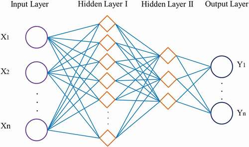
Figure 2. (a) Schematic structure of the TSK fuzzy model. (b) ANFIS model structure (Jang 1993).

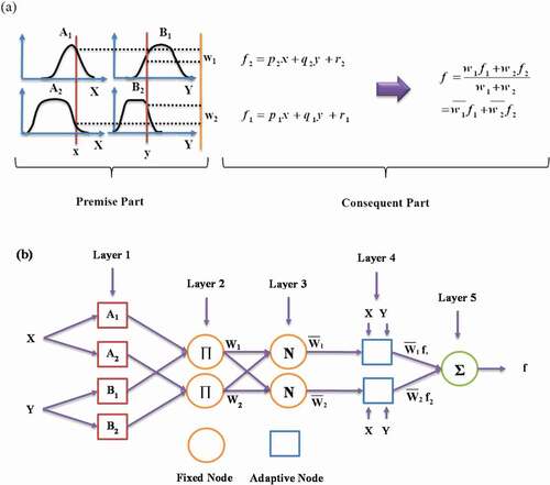
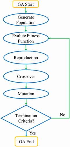
Figure 3. A simple flow sheet of GA (Islam et al. 2016). Simple flow sheet of GA (Martin et al. 2011).

Adaptive Neuro-fuzzy Inference System (ANFIS)

ANFIS is a feed-forward network consists of neural network learning algorithms and fuzzy reasoning to link inputs into outputs, and it was first introduced by Jang (1993). ANFIS is usually used for training purposes to tune the Sugeno Fuzzy Inference System (FIS) to link the inputs and outputs with minimum error. ANFIS uses the least squares estimate (LSE) and gradient descent method as the learning algorithm. It can be employed to construct a set of fuzzy “If–Then” rules with suitable membership functions to create the preliminary input–output pairs. The network consists of nodes with specific functions, or duties, collected in layers with specific functions (Moghaddamnia et al. 2009). A learning phase can be divided into two steps: the first stage involves the propagation of input patterns and applying the iterative least mean square process to assess the optimal resulted parameters, the next stage is to repeat patterns, and then, the back propagation algorithm is employed to adjust the ancestor variables (Shojaeian and Asadizadeh 2020). The structure of the ANFIS system is shown in Figure 6. As shown in this figure, the ANFIS is composed of a network with a five-layer neural structure: the first layer consisting of input nodes, the second layer containing nodes of membership rules or functions, and the third layer representing nodes of the first part of fuzzy rules to calculate the ratio of normalized rules. The fourth layer contains the resulting nodes of the fuzzy rules, and the fifth layer represents the phase of fuzzy decoupling, or output node, which calculates the final output as the sum of all the input signals (Jang 1993).

Genetic Algorithm (GA)

The GA is a stochastic optimization technique and search algorithm developed by Holland (1992). This method is inspired by the evolution of biological species and the mechanism of natural selection, and it is commonly used to provide best solution for search and optimization problems. The GA, which is a member of a wide class of evolutionary algorithms (EA), can provide solutions for optimization issues using techniques inspired by natural evolution concepts, such as inheritance, mutation, selection, and crossover (Martin et al. 2011). As shown in Figure 8, the algorithm starts with the initial population, and its optimal size is dependent on the complexity of the problem (Höglund 2017). As the first-generation size (initial population) is determined, the chromosomes are produced by chance. The selection of the main chromosomes for the production process is done using a roulette wheel.

A cross mechanism combines two selected chromosomes to form two new chromosomes. It is then selected and repeated until a new offspring is generated. The next step is called crossover, and the main step is that the genetic algorithm combines genetic data from two parents to produce new offspring in the production process (Shojaeian and Asadizadeh 2020). Another key parameter of the genetic algorithm is the mutation rate, which is used to maintain the genetic truth from one generation of chromosomes to the next. One or more gene values in a chromosome can change using the mutation process. As the new population has been created, the fitness function for the chromosomes is checked and the selection process will start. The evolutionary process then goes on until the best solution to the problem is obtained (Momeni et al. 2014).

Particle Swarm Optimization (PSO)

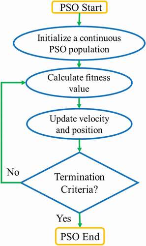
PSO is a metaheuristic and population-based approach that iteratively searches to find a better possible solution by an optimization process (Huang et al. 2020). In this approach, particles move in a multidimensional search space to find the best solution. Therefore, in any optimization issue, many particles should be generated and distributed in the search space (Hajihassani et al. 2015). The main drawback of PSO is its slow converging, but it is very appropriate for searching local extremums (Victoire and Jeyakumar 2004). The position of the particles in the search space changes based on their history and their adjacent particles.

A population, which is literary known as a swarm, would be created by the particles. The simple flow of the PSO algorithm is shown in Figure 4.

Figure 4. Flow diagram of the particle swarm (Ayd et al. 2013).

Differential Evolution (DE)

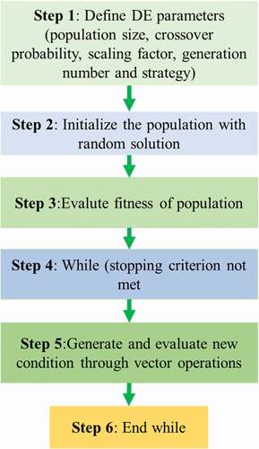
The DE algorithm was introduced by Price and Storn (1997) on the bases of vector operations to produce possible solution to resolve optimization issues. User friendly, simple structure, robustness, escaping from local optimal and speed are the main benefits of this method. The critical action behind this algorithm is a plan for producing trial variable vectors. The main controlling parameters in DE are the number of population (N), probability of crossover (CR) and scaling factor (F). The main stages of the DE algorithm are illustrated in Figure 5.

Figure 5. Differential evolution algorithm (Selvadurai and Głowacki 2008).

Ant Colony optimization (ACO)

The ant colony optimization that was introduced by Sanchez-Ruiz, Gonzalez-Calero, and Diaz-Agudo (2007) is based on the food searching habit of ant colonies. One of the most important features of this algorithm is adopting indirect communication experiences of ants using pheromone paths to search for optimal trials in a problem. The pheromone paths are numerical data converted by ants; these data mirror the experiences of ants while resolving a special issue. This state-of-the-art algorithm has been adopted to solve various problems, particularly problems that require the shortest path to be identified (Zhang et al. 2013).

GDP_MS Modeling

In this paper, ANN, ANFIS-PSO, ANFIS-GA, ANFIS-E and ANFIS-ACO models are employed and proposed to estimate GDP_MS of different countries, which the mining sector contributes to their GDP. An appropriate selection of input data for training and testing of the models is crucial. In this study, 87 data arrays were selected for models, virtually 71% of which for training and the other for testing the models. In this research, testing and training data sets were chosen randomly. In order to have an effective training phase in soft computing methods, normalization of data sets was carried out to the domain of [0,1] by Equation (1)(1) $x_{\mathrm{N}\mathrm{o}\mathrm{r}\mathrm{m}\mathrm{a}\mathrm{l}\mathrm{i}\mathrm{z}\mathrm{e}\mathrm{d}}=\frac{x-x_{Min}}{x_{Max}-x_{Min}}$(1) (Jahed Armaghani et al. 2016).

(1) $x_{\mathrm{N}\mathrm{o}\mathrm{r}\mathrm{m}\mathrm{a}\mathrm{l}\mathrm{i}\mathrm{z}\mathrm{e}\mathrm{d}}=\frac{x-x_{Min}}{x_{Max}-x_{Min}}$(1)

in which x is an input variable and $x_{Min}$ and $x_{Max}$ are minimum and maximum amounts of each variable, respectively. Development of these suggested models is outlined in the following sub-sections.

ANN Modeling

In this research, a multi-layer perceptron ANN, which is known as MLP ANN, was employed to predict GDP_MS. The number of hidden neurons was calculated by trial and error. The proposed network has three inputs in first layer, six neurons in hidden layer and 1 neuron in output layer. The characteristics of the trained network are presented in Table 3.

Table 3. Information of optimum network architecture

Number of input neurons	3
Number of hidden layers	1
Number of hidden neurons	6
Number of output neurons	1
Number of training epochs	300
Number of training datasets	39
Number of testing datasets	16
Training function	Levenberg-Marquardt
Transfer function	TANSIG
Learning rate	0.1
Error goal	0

ANFIS-GA/PSO/DE/ACOR Modeling

In these approaches, GDP_MS is predicted by the ANFIS, and in order to train the ANFIS model, PSO, GA, DE and ACO learning algorithms are adopted separately to achieve a good performance as well as high accuracy. The data array presented in Table 2 is employed to train the ANFIS model utilizing PSO, GA, DE and ACO algorithms. The suggested ANFIS structure has three inputs and one output. The PSO/GA/DE/ACO-based ANFIS approaches are implemented using a program. The program model GDP_MS based input variable geometries. In these approaches, the purpose of PSO/GA/DE/ACO defined in prior section is performed to obtain the optimum parameters of the ANFIS model. Finally, when the learning phase was completed, the optimum amounts of PSO/GA/DE/ACO-based ANFIS model parameters to forecast GDP_MS are given in Table 4.

Table 4. The optimum values of ANFIS-PSO/GA/DE/ACO

Parameter (ANFIS)	Description/ value
Fuzzy structure	Sugeno-type
Type of membership function of the input	Gaussian (“gaussmf”)
Type of membership function of the output	Linear
The center of the cluster influence	0.7
Input number	3
Output number	1
Optimization approach	PSO/GA/DE/ACO
Iteration number	1000
No. of data for training	65
No. of data for test	28
Initial step size	0.3
Step size of decrease rate	0.9
Step size of increase rate	1.10
Number of fuzzy rules	6
Parameter (GA)	Description/ value
Population size	50
Mutation rate	0.05
Crossover	0.7
Parameter (PSO)	Description/ value
Population size	50
W	0.5
C1	2
C2	2
Parameter (DE)	Description/ value
Generation number	50
Population size Np	50
Mutation rate	0.05
Cross probability Cr	0.5
Parameter (ACO)	Description/ value
Initial pheromone matrix value	0.001
Number of construction steps	80
Movement steps	700
Pheromone decay coefficient	0.5

Verification of the Proposed Models

In order to verify the proposed ANN, ANFIS-PSO, ANFIS-GA, ANFIS-E and ANFIS-ACO models, their outputs have been investigated in comparison with real data. The evaluation data (24 data series), which was not used in the models’ construction, was employed for this verification. The prediction performance and ability of the suggested models are controlled based on the evaluation data. For this aim, four statistical indices (SIs) comprising correlation coefficient (R), mean absolute error (MAE), mean square error (MSE) and variance account for VAF were employed and computed for each model. The R index indicates the correlation between the models’ outputs and experimental datasets. On the other hand, the MSE and MAE indices the models’ error compared to the real measured values. Finally, the difference amount between the variances of the experimental datasets and the model outputs are calculated by the VAF index. In general, the higher values of R and VAF (nearer to 100%) and lower amount of the MSE and MAE (near to zero) revealed better performance and capability of the model. These equations are utilized to calculate the above-mentioned indices:

(2) $R=100\left[\frac{\sum _{i=1}^n(A_{ipred}-{\bar{A}}_{pred})(A_{imeas}-{\bar{A}}_{meas})}{\sqrt{\sum _{i=1}^n{(A_{ipred}-{\bar{A}}_{pred})}^2\sum _{i=1}^n{(A_{imeas}-{\bar{A}}_{meas})}^2}}\right]$(2)

(3) $MSE=\frac{1}{n}\sum _{i=1}^n(A_{imeas}-A_{ipred}{)}^2$(3)

(4) $MAE=\frac{\sum _{i=1}^n\left|(A_{imeas}-A_{ipred})\right|}{n}$(4)

(5) $VAF=100(1-\frac{var(A_{imeas}-A{\hspace{0.17em}}_{ipred})}{var(A_{imeas})})$(5)

where n is the dataset number, ${\bar{A}}_{imeas}$ is the average of the measured datasets, ${\bar{A}}_{ipred}$ is the average of the predicted datasets and $A_{imeas}$ and $A_{ipred}$ are the ith measured in laboratory and predicted by models’ components, respectively.

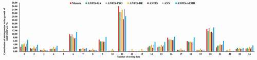
Based on the 24 evaluation data series, the prior mentioned statistical indices were calculated for all of the suggested models and presented in Table 5. As shown in Table 5, the performance of the proposed intelligent models in terms of R, MSE, MAE and VAF is much more than the statistical model. However, the accuracy of the hybrid models (ANFIS-GA/PASO/DE) is somewhat better than that of the other models. In addition, the performance ANFIS-GA is better than the other one. For more evaluation, correlation between the measured data and estimated ones from the ANFIS-GA, ANFIS-PSO, ANFIS-DE, ANFIS, ANN and ANFIS-ACOR models is demonstrated in Figures 6-11, respectively. This comparison also proved that the results of the suggested hybrid intelligent models except ANFIS-ACOR are more associated with the measured data compared to the other models and their results are virtually close to each other. Finally, comparison of the suggested models results with the measured evaluation datasets is depicted in Figure 12, which verified the prediction capabilities of the proposed hybrid intelligent models.

Table 5. Comparing the proposed models performances using the computed statistical indices

Index	ANFIS-GA	ANFIS-PSO	ANFIS-DE	ANFIS	ANN	ANFIS-ACOR
R^2	0.9902	0.9852	0.9829	0.9822	0.9754	0.8907
RMSE	0.9275	0.9044	1.1986	1.7292	1.0434	2.0917
MAE	0.5972	0.4702	1.1188	0.7732	0.7626	1.4402
VAF	97.4381	96.6767	94.9880	89.6910	95.2794	85.7067

Figure 6. Correlation between the ANFIS-GA model outputs and experimental data.

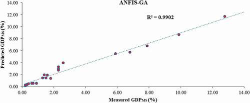
Figure 7. Correlation between the ANFIS-PSO model outputs and experimental data.

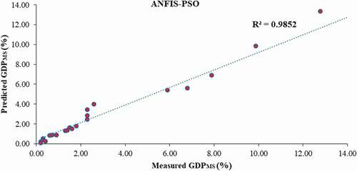
Figure 8. Correlation between the ANFIS-DE model output and experimental data.

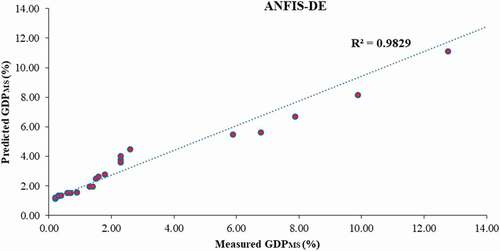
Figure 9. Correlation between the ANFIS model output and experimental data.

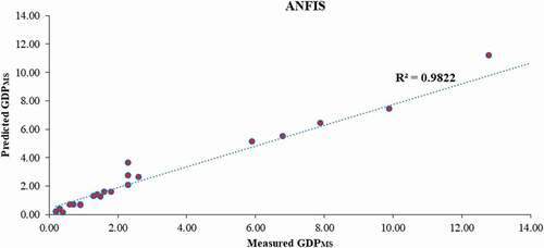
Figure 10. Correlation between the ANN model outputs and experimental data.

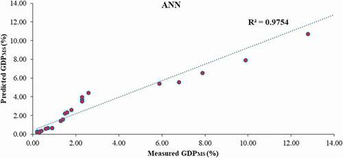
Figure 11. Correlation between the ANFIS-ACOR model output and experimental data.

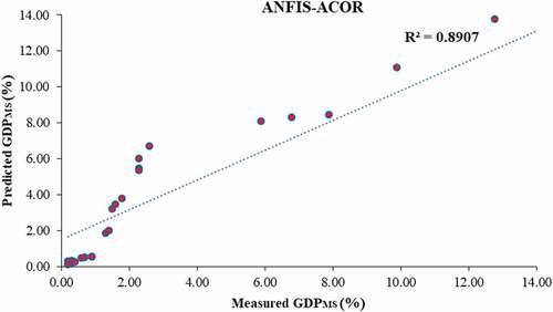
Figure 12. Comparing the suggested models results with the measured evaluation datasets.

Multiple Parametric Sensitivity Analysis (MPSA)

A parametric study was conducted on the models’ outputs to discover the input variables that have the highest influence on the average output variables. The following steps presented in Figure 13 may be followed for a certain set of parameters to apply MPSA to a model output.

Figure 13. Multiple Parametric Sensitivity Analysis algorithm (Correa et al. 2005).

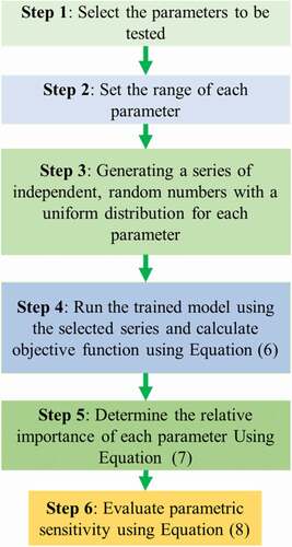
The sum of square errors between the observed and modeled values has been used to evaluate the objective function..

(6) $f_h=\sum _{i=1}^k{\left[x_{0,h}-x_{c,h}(i)\right]}^2$(6)

where $f_h$ is the objective function value for a specific GDP_MS variable h, $x_{0,h}$ is the observed value at this variable, $x_{c,h}(i)$ is the computed value $x_c$ for variable h for each input series, and k isthe number of variables contained in the random series. The range used for each parameter to be evaluated is presented in Table 6. Monte Carlo simulation was applied to generate 24 random numbers for each parameter. In each run of the model, the generated numbers for one variable were applied to the trained models. The relative importance of each parameter independently was evaluated using the following equation:

(7) ${\delta }_h=\frac{f_h}{x_{0,h}}$(7)

Table 6. γ index for model parameter sensitivity (Correa et al. 2005)

γ index	Model parameter sensitivity
$\gamma \le 1$	Insensitive
$1<\gamma \le 100$	Sensitive
$\gamma >100$	Highly sensitive

in which h introduces each pair input. By applying the described procedure to the GDP_MS model, the results were obtained for each evaluated parameter. These results were obtained using (7). The relative importance of each parameter is calculated using following equation:

(8) $\gamma =\sum _{h=1}^{i_{CMSGDP,max}}{\delta }_h$(8)

where the GDP_MS is evaluated from h = 1 (the first series of data) to the maximum value ($i_{CMSGDP,max}$), which is equal to 24 for this model.

For each parameter, the higher the value of the γ index, the more sensitive the GDP_MS model is to this parameter. According to the γ index, the following calcification for model parameter sensitivity has been presented:

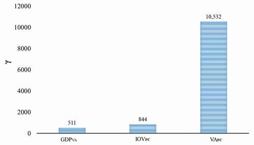
The calculated γ index for GDP_MS model is presented in Figure 14. According to this sensitivity analysis, the GDP_MS model is highly sensitive to all three input parameters and VA_PC and GDP_VA have the highest and the least effect on the GDP_MS model, respectively.

Figure 14. The effect of each input parameter on GDP_MS according to γ index.

Conclusion

In this research, heuristic approaches were applied to predict the contribution of the mining sector to the gross domestic product index (GDP_MS). The influence of three parameters, namely, value added of GDP (GDP_VA), the value of industrial output per capita (IOV_PC) and added value per capita (AV_PC) on GDP_MS, was investigated using heuristic methods such as ANN and ANFIS models as well as for newly hybrid intelligent models (ANFIS-PSO, ANFIS-GA, ANFIS-DE and ANFIS-ACOR). The models’ construction and evaluation were made on the basis 87 pair data gathered form all electronic resources. To verify the new hybrid intelligent models, their achieved results were compared with measured evaluation data using the R, MSE, MAE and VAF indices. This comparison proved that the ANFIS-GA model performance is virtually higher than those of the other models. The hybrid models of PSO and DE are in next order. Moreover, the simulation results of the new hybrid intelligent models are in extremely close accordance with real gathered data. As the last step of the modeling, sensitivity analysis was carried out using the best model and discovered that GDP_MS is highly sensitive to all parameters [i.e., value added of mining resources (GDP_VA), the value of industrial output per capita (IOV_pc), per capita value added (VA_PC)]; also, it was concluded that GDP_MS is more sensitive to VA_PC and less sensitive to GDP_VA among input variables.

Disclosure statement

No potential conflict of interest was reported by the authors.

Correction Statement

This article has been republished with minor changes. These changes do not impact the academic content of the article.

References

- Anghelache C., Manole A., Anghel M. G., Anghel G. 2015. Analysis of final consumption and gross investment influence on GDP – multiple linear regression model. Theor Appl Econ 22:137–42.
- Armeanu D, Andrei J V, Lache L, Panait M. 2017. A multifactor approach to forecasting Romanian gross domestic product (GDP) in the short run. PLoS One 12:1–23. https://doi.org/https://doi.org/10.1371/journal.pone.0181379
- Astakhova N, Demidova L, Nikulchev E, Pluzhnik E. 2015. Forecasting of Time Series ’ Groups with Application of Fuzzy c-Mean Algorithm and Forecasting Models on the Base of Strictly Binary Trees and Modified Clonal 2015:861–73
- Ayd, M., C. Karakuzu, and M. Uçar. 2013. Prediction of surface roughness and cutting zone temperature in dry turning processes of AISI304 stainless steel using ANFIS with PSO learning. Int J Adv Manuf Technol 67, 957–967 (2013). https://doi.org/https://doi.org/10.1007/s00170-012-4540-2
- Camacho M, Dal Bianco M, Martinez-Martin J. 2015. Short-run forecasting of Argentinian gross domestic product growth. Emerg Mark Financ Trade 51:473–85. https://doi.org/https://doi.org/10.1080/1540496X.2015.1025668
- Chai S. H., Lim J. S. 2016. Forecasting business cycle with chaotic time series based on a neural network with weighted fuzzy membership functions. Chaos, Solitons and Fractals :1–9. https://doi.org/https://doi.org/10.1016/j.chaos.2016.03.037
- Chen S., Huang J. .2018. Forecasting China’s primary energy demand based on an improved AI model. Chinese J Popul Resour Environ 16:36–48. https://doi.org/https://doi.org/10.1080/10042857.2018
- Christofides, C., T. S. Eicher, C. Papa-, C. Christofides, and T. S. Eicher. 2015. Author ’ s accepted manuscript did established early warning signals predict the 2008 crises ?*. European Economic Review. doi:https://doi.org/10.1016/j.euroecorev.2015.04.004.
- Cicceri, G., G. Inserra, and M. Limosani. 2020. A machine learning approach to forecast economic recessions-an Italian case study. Mathematics 8:1–20. doi:https://doi.org/10.3390/math8020241.
- Clements, M. P., A. B. Galvão. 2017. Predicting early data revisions to U.S. GDP and the effects of releases on equity markets. Journal of Business & Economic Statistics 35(3):389-406. doi: https://doi.org/10.1080/07350015.2015.1076726
- Correa, J. M., F. A. Farret, V. A. Popov, M. G. Simoes, J. M. Corrêa, S. S. Member. 2005. Sensitivity analysis of the modeling parameters used in simulation of proton exchange membrane fuel cells. IEEE Transactions on Energy Conversion 20:211–18. doi:https://doi.org/10.1109/TEC.2004.842382.
- Díaz-Rodríguez, P., J. C. Cancilla, G. Matute, and J. S. Torrecilla. 2015. Viscosity estimation of binary mixtures of ionic liquids through a multi-layer perceptron model. Journal of Industrial and Engineering Chemistry 21:1350–53. doi:https://doi.org/10.1016/j.jiec.2014.06.005.
- Hajihassani, M., D. Jahed Armaghani, M. Monjezi, E. T. Mohamad, and A. Marto. 2015. Blast-induced air and ground vibration prediction: A particle swarm optimization-based artificial neural network approach. Environmental Earth Sciences 74 (4):2799–817. doi:https://doi.org/10.1007/s12665-015-4274-1.
- Höglund, H. 2017. Tax payment default prediction using genetic algorithm-based variable selection. Expert Systems with Applications 88:368–75. doi:https://doi.org/10.1016/j.eswa.2017.07.027.
- Holland, J. H. 1992. Adaptation in natural and artificial systems, vol. 1. The MIT Press. https://direct.mit.edu/books/book/2574/Adaptation-in-Natural-and-Artificial-SystemsAn
- Huang, J., P. G. Asteris, S. Manafi Khajeh Pasha, A. S. Mohammed, and M. Hasanipanah. 2020. A new auto-tuning model for predicting the rock fragmentation: A cat swarm optimization algorithm. Engineering with Computers 1–12. doi:https://doi.org/10.1007/s00366-020-01207-4.
- Islam, S. M. Mohandes, S. Rehman, 2016. Vertical extrapolation of wind speed using artificial neural network hybrid system. Neural Computing and Applications 28:2351–2361. https://doi.org/10.1007/s00521-016-2373-x
- Jahed Armaghani, D., E. Tonnizam Mohamad, M. Hajihassani, S. V. Alavi Nezhad Khalil Abad, A. Marto, and M. R. Moghaddam. 2016. Evaluation and prediction of flyrock resulting from blasting operations using empirical and computational methods. Engineering with Computers 32 (1):109–21. https://doi.org/https://doi.org/10.1007/s00366-015-0402-5.
- Jang, J.-S. 1993. ANFIS: Adaptive-network-based fuzzy inference system. IEEE Transactions on Systems, Man, and Cybernetics 23 (3):665–85. doi:https://doi.org/10.1109/21.256541.
- Junoh, M. 2004. Predicting GDP growth in malaysia using knowledge-based economy indicator: A comparison between neural network and econometric approach. Sunw Coll J 1:39–50.
- Karaca, Y., Ş. Bayrak, and E. F. Yetkin. 2017. The Classification of Turkish Economic Growth by Artificial Neural Network Algorithms. In: Gervasi O. et al. (eds) Computational Science and Its Applications – ICCSA 2017. ICCSA 2017. Lecture Notes in Computer Science, vol 10405. Springer, Cham. https://doi.org/https://doi.org/10.1007/978-3-319-62395-5_9
- Kreinovich V, Sriboonchitta S, Chakpitak N. 2017. Predictive Econometrics and Big Data :19. https://doi.org/https://doi.org/10.1007/978–3–319–70942–0
- Kuosmanen, P., Vataja J. .2018. Time-varying predictive content of financial variables in forecasting. Q Rev Econ Financ. https://doi.org/https://doi.org/10.1016/j.qref.2018.08.002
- Kurihara, Y., and A. Fukushima. 2019. AR model or machine learning for forecasting GDP and consumer price for G7 countries. Applied Economics and Finance 6 (3):1. doi:https://doi.org/10.11114/aef.v6i3.4126.
- Kyo K, Noda H. 2018. A Bayesian Approach for Analyzing the Dynamic Dependence of GDP on the Unemployment Rate in Japan. International Journal of Modeling and Optimization 8:55–61. https://doi.org/https://doi.org/10.7763/ijmo.2018.v8.624
- Leader, T. 2017. Annual economic report (2016). Tajikistan. vol. 1.
- Leigh, J. P., and J. Du. 2015. Brief report: Forecasting the economic burden of autism in 2015 and 2025 in the United States. Journal of Autism and Developmental Disorders 45 (12):4135–39. doi:https://doi.org/10.1007/s10803-015-2521-7.
- Lu, X., M. Hasanipanah, K. Brindhadevi, H. Bakhshandeh Amnieh, and S. Khalafi. 2020. ORELM: A novel machine learning approach for prediction of flyrock in mine blasting. Natural Resources Research 29 (2):641–54. doi:https://doi.org/10.1007/s11053-019-09532-2.
- Martin, A., V. Gayathri, G. Saranya, P. Gayathri, and P. Venkatesan. 2011. A hybrid model for bankruptcy prediction using genetic algorithm,Fuzzy C-Means and Mars. International Journal on Soft Computing 2 (1):12–24. doi:https://doi.org/10.5121/ijsc.2011.2102.
- Mataloni, L. 2017. OECD. OECD Economic Survey. http://www.oecd.org.
- Moghaddamnia, A., M. Ghafari Gousheh, J. Piri, S. Amin, and D. Han. 2009. Evaporation estimation using artificial neural networks and adaptive neuro-fuzzy inference system techniques. Advances in Water Resources 32 (1):88–97. doi:https://doi.org/10.1016/j.advwatres.2008.10.005.
- Momeni, E., R. Nazir, D. Jahed Armaghani, and H. Maizir. 2014. Prediction of pile bearing capacity using a hybrid genetic algorithm-based ANN. Measurement 57:122–31. doi:https://doi.org/10.1016/j.measurement.2014.08.007.
- Nikafshan Rad, H., I. Bakhshayeshi, W. A. Wan Jusoh, M. M. Tahir, and L. K. Foong. 2020. Prediction of flyrock in mine blasting: A new computational intelligence approach. Natural Resources Research 29 (2):609–23. doi:https://doi.org/10.1007/s11053-019-09464-x.
- OECD. 2017. México. OECD Economic Surveys 46. https://doi.org/https://doi.org/10.1787/eco_surveys-mex-2017-en
- Price, K., and R. Storn. 1997. Differential evolution – a simple and efficient heuristic for global optimization over continuous spaces. Journal of Global Optimization 341–59. doi:https://doi.org/10.1023/A:1008202821328.
- Proietti T., Marczak M., Mazzi G. 2017. Euro mind- D: A Density Estimate of Monthly Gross Domestic Product for the Euro Area. Journal of Applied Econometrics 32:683–703. https://doi.org/https://doi.org/10.1002/jae.2556
- Rakic G., Markovic S., Jovic S., et al .2018. Analysing of exchange rate and gross domestic product (GDP) by adaptive neuro-fuzzy inference system (ANFIS). Physica A: Statistical Mechanics and its Applications 513:333–338. https://doi.org/https://doi.org/10.1016/j.physa.2018.09.009
- Ramírez, K. M., J. M. Hormaza, and S. V. Soto. 2020. Artificial intelligence and its impact on the prediction of economic indicators. ACM International Conference Proceedings Series. doi:https://doi.org/10.1145/3410352.3410827.
- Rezaei, M., and M. Asadizadeh. 2020. Journal of Mining and Environment (JME) predicting unconfined compressive strength of intact rock using new hybrid intelligent models. Journal of Mining Environment 11:231–46. doi:https://doi.org/10.22044/jme.2019.8839.1774.
- Sanchez-Ruiz, A. A., P. A. Gonzalez-Calero, and B. Diaz-Agudo. 2007. Combining HTN-DL planning and CBR to compound semantic web services. CEUR Workshop Proceedings 275:104–05. doi:https://doi.org/10.1109/MCI.2006.329691.
- Selvadurai, A. P. S., and A. Głowacki. 2008. Permeability hysterisis of limestone during isotropic compression. Groundwater 46 (1):113–19. doi:https://doi.org/10.1111/j.1745-6584.2007.00390.x.
- Semuel H., Nurina S., Semuel Nurina H. S. 2015. Analysis of the Effect of Inflation, Interest Rates, and Exchange Rates on Gross Domestic Product (GDP) in Indonesia. Proc Int Conf Glob Business, Econ Financ Soc Sci, GB15_Thai Conf :20–2.
- Shojaeian, A., and M. Asadizadeh. 2020. Prediction of surface tension of the binary mixtures containing ionic liquid using heuristic approaches; an input parameters investigation. Journal of Molecular Liquids 298:111976. doi:https://doi.org/10.1016/j.molliq.2019.111976.
- Situation, T. E. 2017. Economics E-Journal. http://www.economics-ejournal.org.
- Song, R., and X. Xue. 2017. Freight volume forecast based on improved radial basis function neural network. Bol Tec Bull 55:419–23.
- Stevanović M, Vujičić S, Gajić A. M. 2018. Gross domestic product estimation based on electricity utilization by the artificial neural network. Physica A: Statistical Mechanics and its Applications 489:28–31. https://doi.org/https://doi.org/10.1016/j.physa.2017.07.023
- Victoire, T. A. A., and A. E. Jeyakumar. 2004. Hybrid PSO–SQP for economic dispatch with valve-point effect. Electric Power Systems Research 71:51–59. doi:https://doi.org/10.1016/j.epsr.2003.12.017.
- Yoon, J. 2021. Forecasting of real GDP growth using machine learning models: gradient boosting and random forest approach. Computational Economics 57:247–65. doi:https://doi.org/10.1007/s10614-020-10054-w.
- Zhang, X., Q. Wang, F. T. S. Chan, S. Mahadevan, and Y. Deng. 2013. A physarum polycephalum optimization algorithm for the bi-objective shortest path problem. International Journal of Unconventional Computing 10:143–62.
- Zhao, W., and D. Niu. 2017. Prediction of CO2emission in China’s power generation industry with Gauss optimized Cuckoo search algorithm and wavelet neural network based on STIRPAT model with ridge regression. Sustain 9. doi:https://doi.org/10.3390/su9122377.
- Zhou, J., N. Aghili, E. N. Ghaleini, D. T. Bui, M. M. Tahir, M. Koopialipoor, and A. Monte. 2020. Carlo simulation approach for effective assessment of flyrock based on intelligent system of neural network. Engineering with Computers 36:713–23. doi:https://doi.org/10.1007/s00366-019-00726-z.