Correlation-augmented Naïve Bayes (CAN) Algorithm: A Novel Bayesian Method Adjusted for Direct Marketing

ABSTRACT

Direct marketing identifies customers who buy, more probable, a specific product to reduce the cost and increase the response rate of a marketing campaign. The advancement of technology in the current era makes the data collection process easy. Hence, a large number of customer data can be stored in companies where they can be employed to solve the direct marketing problem. In this paper, a novel Bayesian method titled correlation-augment naïve Bayes (CAN) is proposed to improve the conventional naïve Bayes (NB) classifier. The performance of the proposed method in terms of the response rate is evaluated and compared to several well-known Bayesian networks and other well-known classifiers based on seven real-world datasets from different areas with different characteristics. The experimental results show that the proposed CAN method has a much better performance compared to the other investigated methods for direct marketing in almost all cases.

Introduction

Almost all industries such as banking, insurance, health care, and retailing need marketing and advertisement to sell their goods and services (Ling and Li 1998). There are two common ways to introduce products and services; mass marketing and direct marketing (Nachev and Hogan 2014). In mass marketing, a single message is published to all customers via television, radio, newspaper, and so on (Elsalamony 2014). As companies do not have a direct relationship with customers for new product offers in this strategy, an increase in the number of companies or products leads to a reduction in the efficacy, increase in the cost, and decrease in the response rate of this strategy (Mitik et al. 2017). However, the market is highly competitive where mass marketing campaigns are not very successful and companies focus on direct marketing campaigns to target a specific set of customers (Parlar and Acaravci 2017). In the direct marketing strategy, companies study the characteristics and the needs of potential customers to select a target set of customers. The communication between companies and customers is done by e-mail, phone call, SMS, and post. The goal of the organizations is to increase the response rate of their promotion with a limited budget (Miguéis, Camanho, and Borges 2017).

The advantages and disadvantages of direct marketing have been discussed in some researches. Vriens et al. (1998) emphasized the flexibility of direct mailing in time, model, test, and examination. Verhoef et al. (2003) highlighted the ability to give customized offers to customers and the loss of direct competition for customers’ attention. To show that an increase in the response rate is not easy, but a small improvement can create a significant profit, Baesens et al. (2002) demonstrated that a one percent increase in the response rate could result in an additional relatively large profit. Direct marketing can improve the customers’ loyalty (Sun, Li, and Zhou 2006) while, at the same time, it can result in a negative effect on customers if they receive uninteresting promotions frequently (Ansariet al., 2008).

Nowadays, most companies have a vast amount of data on customers profiles, transactions, and responses to previous products in their databases, where these data can be used to keep relationships with the customers to propose their customized product offer (Ouet al., 2003). Because it is infeasible to analyze the data manually to discover useful patterns for direct marketing (Ling and Li 1998), automated methods should be used to analyze the data in which data mining is considered as one of the strongest. Data mining techniques have a huge potential to discover latent knowledge of databases and can predict potential customers who buy, more probably, a new product (Miguéis, Camanho, and Borges 2017).

Data mining techniques play an essential role in different industries. Nowadays, the advancement of technology makes the data collection process easy. Thus, the problem of organizations is to discover hidden knowledge from large amounts of data in databases. There are several applications of various data mining techniques, including classification, clustering, and association rule mining in different areas (Han, Pei, and Kamber 2011).

The classification technique requires the construction of a classifier to predict the class of new tuples whose class labels are unknown. This prediction is made by finding a model that distinguishes between classes based on a training set with known class labels. The induction of classifiers from the raw data is an important problem in data mining, and hence, numerous solutions such as naïve Bayes, Bayesian networks, decision tree, support vector machines (SVM), logistic regression, extra trees, K-nearest neighbor (KNN), Ada-Boost, and Bagging have been proposed in the literature to solve this problem. In this paper, another classifier titled correlation-augment naïve Bayes (CAN) is proposed to improve the performance of the conventional naïve Bayes (NB) classifier in the direct marketing problem.

The rest of the paper is organized as follows: the literature of the subject is reviewed in Section 2. The competing Bayesian methods are presented in Section 3. The details of the proposed CAN method are provided in Section 4. In Section 5, the performance of the proposed method is evaluated and compared to other existing methods based on seven real-world datasets. Finally, the concluding remarks are provided in Section 6.

Literature Review

Data mining techniques are widely used to improve the performance of companies in several contexts by discovering valuable hidden knowledge from a massive volume of raw data (Burton et al. 2014; Chen, Fan, and Sun 2015; Seret, Bejinaru, and Baesens 2015). The results obtained from empirical studies emphasize using data mining methods to design a direct marketing campaign to predict proper target customers. For instance, Parlar and Acaravci (2017) applied the feature selection method to select important features and improved the marketing models’ processing time and response rate by reducing the number of features. Mitiket al. (2017) used naïve Bayes and decision tree classifiers to identify the customers interested in the offered products and then cluster them for channel suggestions. Miguéiset al. (2017) presented a random forest model to identify the target customers for banking campaigns and compared the under-sampling (the EasyEnsemble) and the over-sampling (the Synthetic Minority Oversampling) techniques as a solution to a class-imbalanced problem. Elsalamony and Elsayad (2013) applied the neural network and the decision tree models on real-world data of deposit campaigns to increase the effectiveness of the campaign. Moro, Cortez, and Rita (2014) introduced four data mining models, including support vector machine, decision tree, neural network, and logistic regression, to increase the response rate of a banking campaign and compared the performance of the models. Tavana et al. (2018) proposed an artificial neural network and Bayesian network for liquidity risk assessment in banking and evaluated their efficiency based on a real-world case study. Beheshtian-Ardakani, Fathian, and Gholamian (2018) proposed a novel method for product bundling and direct marketing in e-commerce. They first grouped the customers by the k-means algorithm and then applied the Apriori algorithm to determine the association rules for each product bundle. Finally, they employed the SVM model to determine which product bundles should be offered to each customer. Dutta, Bhattacharya, and Guin (2015) reviewed 103 research papers on the usage of data mining techniques in market segmentation. They grouped them into 13 methods, including kernel-based, neural network, k-means, RFM analysis, etc. Chen, Sain, and Guo (2012) presented k-means and decision tree approaches, based on RFM models, to segment the customers of an online retailer. Lawi, Velayaty, and Zainuddin (2017) used the Ada-Boost algorithm based on a support vector machine to determine the target customers for direct marketing of a banking campaign. Zakaryazad and Duman (2016) presented a profit-driven artificial neural network with a new penalty function and compared it to three classifier techniques, including naïve Bayes, decision trees, and neural networks. Koumétio, Cherif, and Hassan (2018) presented a new classification technique to optimize the prediction of telemarketing target calls for selling bank long-term deposits. They evaluated and compared their method with Naïve Bayes, Decision Trees, Artificial Neural Network and Support Vector Machines and concluded that their method provides the best performance in terms of f-measure. Coussement, Harrigan, and Benoit (2015) applied the most important classification techniques such as neural network, naïve Bayes, decision tree, KNN, linear and quadratic discriminant, and logistic regression on four real-world datasets and compared their performances. Koumétio and Toulni (2021) tried to optimize the prediction of telemarketing target calls for selling bank long-term deposits in smart cities using improved KNN model and concluded that their approach improves the performance (f1-measure) of other algorithms used, and vary reduced time processing. Darzi, Niaki, and Khedmati (2019) employed several methods to solve the direct marketing problem of the COIL challenge 2000. They presented a hybrid method (Tree-augment naïve Bayes (TAN) + under-sampling) as the best approach to solve this problem.

In this paper, a method called “CAN”is proposed for the direct marketing problem. As a novel Bayesian, this method relaxes the heavy independent assumption of the conventional naïve Bayes classifier. Besides, some other extensions are applied in the proposed method to customize it for direct marketing. As the aim is to assess the performance of the proposed method, its efficacy is compared to the ones of other existing methods introduced in the next section based on seven real-world datasets.

Bayesian Methods

Among different classifiers, the naïve Bayes algorithm is one of the most widely used and successful classification techniques (Coussement, Harrigan, and Benoit 2015), flexible for dealing with a different number of features or classes, and works well with databases containing noisy data (Ratanamahatana and Gunopulos 2002). Furthermore, despite the simplicity, the naïve Bayes algorithm is one of the fastest learning algorithms competitive with sophisticated classifiers (Friedman, Geiger, and Goldszmidt 1997). In the next subsections, a brief explanation of five Bayesian methods, including naïve Bayes (NB), tree-augment naïve (TAN) Bayes, sequential forward selection and joining (FSSJ), backward sequential elimination and joining (BSEJ), and averaged one-dependence estimators (AODE) is presented.

Naïve Bayes algorithm

Abstractly, the naïve Bayes classifier is a conditional probability model. Let $X=\left(a_1,a_2,\dots ,a_n\right)$ be a sample of a test dataset where, $a_j;j=1,2,\dots ,n$ represents the value of an attribute $A_j$. The Bayesian algorithm assigns the sample $X$ to class $C$ when the value associated with the class $C$ is the maximum posterior class probability, $P(clas{s}_C|X)$, given in Equation (1)(1) $P\left(Clas{s}_C|X\right)=\underset{k}{Max}\left\{P\left(Clas{s}_k|X\right)\right\}$(1) .

(1) $P\left(Clas{s}_C|X\right)=\underset{k}{Max}\left\{P\left(Clas{s}_k|X\right)\right\}$(1)

This conditional probability can be formulated based on the Bayes theorem presented in Equation (2)(2) $P\left(Clas{s}_k|X\right)=\frac{P\left(X|Clas{s}_k\right)\ast P\left(Clas{s}_k\right)}{P\left(X\right)}$(2) .

(2) $P\left(Clas{s}_k|X\right)=\frac{P\left(X|Clas{s}_k\right)\ast P\left(Clas{s}_k\right)}{P\left(X\right)}$(2)

In the naïve Bayesian algorithm, it is assumed that the attributes are independent, and hence, as shown in Figure 1, each attribute has one arc that is connected to the class variable. Due to the independence assumption, the conditional probability in Equation (2)(2) $P\left(Clas{s}_k|X\right)=\frac{P\left(X|Clas{s}_k\right)\ast P\left(Clas{s}_k\right)}{P\left(X\right)}$(2) can be obtained easily, based on Equation (3)(3) $P\left(a_1,a_2,\dots ,a_n|Clas{s}_k\right)=\prod _{j=1}^{n}P\left(a_j|Clas{s}_k\right)$(3) .

(3) $P\left(a_1,a_2,\dots ,a_n|Clas{s}_k\right)=\prod _{j=1}^{n}P\left(a_j|Clas{s}_k\right)$(3)

Figure 1. An example of the NB network.

Besides, as $P\left(X\right)$ is fixed for all classes, the naïve Bayes classifier can be obtained, finally, based on the following equation:

(4) $P\left(Clas{s}_C|X\right)=\underset{k}{Max}\left\{P\left(Clas{s}_k\right)\ast \prod _{j=1}^{n}P\left(a_j|Clas{s}_k\right)\right\}.$(4)

As mentioned above, the naïve Bayes classification model works under the assumption of independent attributes. This assumption is often violated in reality, which leads to poor performance on some datasets (Pazzani 1996). Moreover, in many situations, such as in the direct marketing problem, the distribution of the classes of the target attribute is highly unbalanced; that is, most of the tuples belong to one class, and the rest that is so small, belongs to the other class. In these situations, most of the classification methods, including the naïve Bayes classifier, tend to bias toward the majority class, while it is more important to identify the minority classes correctly. As a result, some methods were proposed in the literature to relax its independence assumption to improve its performance. In the following subsections, some well-known Bayesian networks that relax the independence assumption of the naïve Bayes method are introduced.

Tree-augment Naïve Bayes (TAN)

TAN uses a tree construction, in which the attributes can be connected (Friedman, Geiger, and Goldszmidt 1997). The class-label attribute variable does not have parents in the TAN network, while the other attributes are connected to the class label attribute. Further, the attributes are connected, at most, to one other attribute as their parent. An example of the TAN network is shown in Figure 2.

Figure 2. An example of the TAN network: the class node C has no parents, feature nodes have two parents including the class node and one feature node, the node $A_1$ as the root of the features’ tree, which has only the class node as a parent (De Campos et al. 2016; Darzi et al. 2020).

The learning procedure of the TAN network is based on the well-known method reported by Chow and Liu (1968) as follows:

1. Compute the mutual information ($I_p$) between each pair of attributes based on Equation (5)(5) $I_p\left(X;Y|Z\right)=\sum _{x,y,z}P\left(x,y,z\right)log\frac{P\left(x,y|z\right)}{P\left(x|z\right)P\left(y|z\right)}$(5) . This equation measures the information that $Y$ provides about $X$ when the value of $Z$ is known.

(5) $I_p\left(X;Y|Z\right)=\sum _{x,y,z}P\left(x,y,z\right)log\frac{P\left(x,y|z\right)}{P\left(x|z\right)P\left(y|z\right)}$(5)

1. Build a complete undirected graph in which the vertices are the attributes in $X$. The edges are weighted according to the pairwise mutual information.

2. Build a maximum weighted spanning tree.

3. Transform the resulting undirected graph to a directed graph by selecting the class-label attribute as the root node and setting the direction of all edges outward from it.

4. Construct a TAN model by adding an arc from the class-label attribute to all other attributes (Darzi, Niaki, and Khedmati 2019).

The TAN algorithm changes the class probability of the naïve Bayes given in Equations(4)(4) $P\left(Clas{s}_C|X\right)=\underset{k}{Max}\left\{P\left(Clas{s}_k\right)\ast \prod _{j=1}^{n}P\left(a_j|Clas{s}_k\right)\right\}.$(4) to (6) as:

(6) $P\left(Clas{s}_C|X\right)=\underset{k}{Max}\left\{\theta \ast P\left(Clas{s}_k\right)\ast \prod _{j=1}^{n}P\left(a_j|Parents\left(a_j\right)\right)\right\}$(6)

where θ is the normalization constant, $P\left(Clas{s}_k\right)$ is the prior probability for Class $k$, and $Parents\left(a_j\right)$ is the set of direct parents for node $a_j$.

Forward Sequential Selection and Joining (FSSJ)

FSSJ improves the Bayesian classifier by searching for dependencies among the attributes. This classifier searches for a typical local where the objective function is accurate (Blanco et al. 2005). The FSSJ algorithm uses the set of attributes to be used by the Bayesian classifier. It starts with an empty set and then employs two operators to create a new combination of the attributes. As a result, a new classifier is generated at each iteration. The general steps involved in the FSSJ classifier are as follows:

1. Add a new attribute $X_{new}$ (not in the attribute list) conditionally independent of all other attributes used in the classifier.

2. Join $X_{new}$ with each attribute currently used by the classifier.

3. Repeat the above modifying procedure until no improvement can be obtained.

Backward Sequential elimination and Joining (BSEJ)

The BSEJ algorithm generates a Bayesian classifier considering all the attributes as conditionally independent. It uses the following two operators:

1. Replace each pair of attributes used by the classifier with a new attribute that joins the pair of attributes.

2. Delete each attribute used by the classifier.

Like the FSSJ, the BSEJ algorithm considers all one-step modifications until no improvement is reachable.

A Bayesian network of the above two methods is presented in Figure 3.

Figure 3. An example of the FSSJ and the BSEJ network: They do not limit the number of parents, but sub-graphs of the connected nodes must be complete (sub-graphs in Figure (3) are $\{A_1,A_2\}$ and $\{A_4,A_5,A_6\}$). Also, the nodes are permitted to be deleted ($A_3$ is deleted). $A_7$ is neither deleted nor connected to other nodes (Mihaljević, Bielza, and Larrañaga 2018).

The FSSJ and BSEJ algorithms classify the samples based on Equation (7)(7) $\underset{k}{Max}\left\{P\left(Clas{s}_k\right)\ast \prod _{i=1}^{g_h}P\left(joine{d}_{g_i}|Clas{s}_k\right)\ast \prod _{j=1}^{s_p}P\left(x_{sj}|Clas{s}_k\right)\right\}$(7) , where the resulting attribute set is obtained as the Cartesian product of the attributes shown as {$joine{d}_{g_1},joine{d}_{g_2},\dots ,joine{d}_{g_h}$}. In Figure 3, this set is $\{({\mathrm{A}}_1,{\mathrm{A}}_2),({\mathrm{A}}_4,{\mathrm{A}}_5,{\mathrm{A}}_6)\}$. The rest of the original attributes that have been neither deleted nor joined are shown as {$x_{s1},x_{s2},\dots ,x_{sp}$}. In Figure 3, this set is {${\mathrm{A}}_7$} (Interested readers are referred to Pazzani (1996) for more details).

$P\left(Clas{s}_C|X\right)=$

(7) $\underset{k}{Max}\left\{P\left(Clas{s}_k\right)\ast \prod _{i=1}^{g_h}P\left(joine{d}_{g_i}|Clas{s}_k\right)\ast \prod _{j=1}^{s_p}P\left(x_{sj}|Clas{s}_k\right)\right\}$(7)

Averaged One-dependence Estimators (AODE)

AODE relaxes the independence assumption by averaging over all models in which each attribute is connected to the class node and another single node. An example of the AODE network is shown in Figure 4.

Figure 4. An example of the AODE network.

In the AODE method, Equation (8)(8) $P\left(y|x\right)=\frac{P\left(y,x\right)}{P\left(x\right)}\propto P\left(y,x\right)$(8) is first obtained based on conditional probability.

(8) $P\left(y|x\right)=\frac{P\left(y,x\right)}{P\left(x\right)}\propto P\left(y,x\right)$(8)

Then, using the product rule (Webb, Boughton, and Wang 2005), the following equation is obtained for each value of attribute $x$:

(9) $P\left(y,x\right)=P\left(y,x_i\right)P\left(x|y,x_i\right)$(9)

where $x_i$ is the value of the $i^{th}$ attribute. Next, the mean over any group of attribute values is obtained for any $I\subseteq \left\{1,2,\dots ,n\right\}$ based on Equation (10):

(10) $P\left(y,x\right)=\frac{{\sum }_{i\in I}P\left(y,x_i\right)P\left(x|y,x_i\right)}{\left|I\right|}$(10)

As a result, we have:

(11) $P\left(y,x\right)=\frac{{\sum }_{i:1\le i\le n\wedge F(x_i)\ge m}p(y,x_i)p(x|y,x_i)}{\left|\left\{i:1\le i\le n\wedge F(x_i)\ge m\right\}\right|}$(11)

where $F\left(x_i\right)$ is the frequency of attribute-value $x_i$ in the training set. Finally, AODE selects the class that maximizes Equation (12):

(12) $P\left(Clas{s}_C|X\right)=\underset{k}{Max}\left\{\sum { }_{i:1\le i\le n\wedge F\left(x_i\right)\ge m}P\left(Clas{s}_k,x_i\right){\prod }_{j=1}^{n}P\left(x_j|Clas{s}_k,x_i\right)\right\}$(12)

in which $y$ is considered as the target variable and $P(Clas{s}_k|X)$ is the probability that sample $X$ belongs to Class $k$ (see Webb, Boughton, and Wang (2005) for more details).

The next section proposes a new modification to relax the independence assumption involved in the naïve Bayes method to improve its performance.

The Proposed method: Correlation-augment Naïve Bayes (CAN)

In this section, a new method called correlation-augment naïve Bayes (CAN) is proposed to extend the naïve Bayes model that relaxes the independence assumption of the attributes. The probabilities are obtained based on Equation (13)(13) $P\left(a_1,a_2,\dots ,a_n|Clas{s}_k\right)\equiv \prod _{j=1,j\ne s,j\ne t,j\ne \dots }^n\left(k\left(a_j,a_s,a_t,\dots |Clas{s}_k\right)\right)$(13) as a reconstructed and improved version of Equation (3)(3) $P\left(a_1,a_2,\dots ,a_n|Clas{s}_k\right)=\prod _{j=1}^{n}P\left(a_j|Clas{s}_k\right)$(3) in the proposed method. In Equation (13)(13) $P\left(a_1,a_2,\dots ,a_n|Clas{s}_k\right)\equiv \prod _{j=1,j\ne s,j\ne t,j\ne \dots }^n\left(k\left(a_j,a_s,a_t,\dots |Clas{s}_k\right)\right)$(13) , $k\left(a_j,a_s,a_t,\dots |Clas{s}_k\right)$ is the conditional probability of the intersection of attributes $a_j$, $a_s,a_t,\dots$(correlated attributes) plus one (more details are given in Equation (17)(17) $k\left(a_j,a_s,a_t,\dots \right)=1+\frac{count\left(a_j,a_s,a_t,\dots \right)+1}{samplesize}$(17) ).

(13) $P\left(a_1,a_2,\dots ,a_n|Clas{s}_k\right)\equiv \prod _{j=1,j\ne s,j\ne t,j\ne \dots }^n\left(k\left(a_j,a_s,a_t,\dots |Clas{s}_k\right)\right)$(13)

As an example, suppose there exist five attributes in which the attributes $a_2$, $a_3$ and $a_4$ are correlated while attributes $a_1$ and $a_5$ are independent and they are not correlated with other attributes. Then, the probability is obtained as follows:

(14) $P\left(a_1,a_2,\dots ,a_5|Clas{s}_k\right)\equiv k\left(a_1|Clas{s}_k\right)\ast k\left(a_2,a_3,a_4|Clas{s}_k\right)\ast k\left(a_5|Clas{s}_k\right)$(14)

Here, the correlation between the attributes is examined by the Spearman correlation test (Wissler 1905), based on which each attribute is connected to other attributes if their Spearman correlation is bigger than a pre-specified value $\mathrm{P}$, $\left(0\le P\le 1\right)$, as shown in Equation (15)(15) $\mathrm{S}\mathrm{p}\mathrm{e}\mathrm{a}\mathrm{r}\mathrm{m}\mathrm{a}\mathrm{n}cor\left(a_k,a_j\right)\ge \mathrm{P}$(15) .

(15) $\mathrm{S}\mathrm{p}\mathrm{e}\mathrm{a}\mathrm{r}\mathrm{m}\mathrm{a}\mathrm{n}cor\left(a_k,a_j\right)\ge \mathrm{P}$(15)

In the CAN algorithm, an attribute is correlated with a set of attributes if it is correlated with at least one attribute of that set. For example, $a_k$ is correlated with $set\left(a_j,a_s,a_t\right)$ if it satisfies at least one of the conditions specified in Equation (16)(16) $cor\left(a_k,a_j\right)\ge \mathrm{P}\mathbf{o}\mathbf{r}cor\left(a_k,a_s\right)\ge \mathrm{P}\mathbf{o}\mathbf{r}cor\left(a_k,a_t\right)\ge \mathrm{P}$(16) .

(16) $cor\left(a_k,a_j\right)\ge \mathrm{P}\mathbf{o}\mathbf{r}cor\left(a_k,a_s\right)\ge \mathrm{P}\mathbf{o}\mathbf{r}cor\left(a_k,a_t\right)\ge \mathrm{P}$(16)

As mentioned above, compared to the NB network, the CAN network allows more dependencies among the attributes, where an example of its network is presented in Figure 5. From a set of attributes, only one vector is connected to the target variable in the CAN network.

Figure 5. An example of the CAN network.

The CAN method is simpler, and its processing time is expected to be less than the other Bayesian methods, including TAN, FSSJ, BSEJ, and AODE, because

1. The correlation test to build the CAN network is simpler than the ones in the other Bayesian methods, and hence, the processing time is expected to be significantly less

2. The CAN method does not compute the conditional probability shown in Equation (13)(13) $P\left(a_1,a_2,\dots ,a_n|Clas{s}_k\right)\equiv \prod _{j=1,j\ne s,j\ne t,j\ne \dots }^n\left(k\left(a_j,a_s,a_t,\dots |Clas{s}_k\right)\right)$(13) for each node. Instead, it calculates this probability only for each set of correlated attributes. Accordingly, the processing time is expected to be less.

Both the NB and the CAN classifiers require that each conditional probability obtained by Equations(3)(3) $P\left(a_1,a_2,\dots ,a_n|Clas{s}_k\right)=\prod _{j=1}^{n}P\left(a_j|Clas{s}_k\right)$(3) and (13(13) $P\left(a_1,a_2,\dots ,a_n|Clas{s}_k\right)\equiv \prod _{j=1,j\ne s,j\ne t,j\ne \dots }^n\left(k\left(a_j,a_s,a_t,\dots |Clas{s}_k\right)\right)$(13) ) be non-zero; otherwise, the total predicted probability would be zero. Considering the intersection of several probabilities in Equation (13)(13) $P\left(a_1,a_2,\dots ,a_n|Clas{s}_k\right)\equiv \prod _{j=1,j\ne s,j\ne t,j\ne \dots }^n\left(k\left(a_j,a_s,a_t,\dots |Clas{s}_k\right)\right)$(13) , the chance of being zero the probability of $P\left(a_j,a_s,a_t,\dots |Clas{s}_k\right)$ increases compared to Equation (3)(3) $P\left(a_1,a_2,\dots ,a_n|Clas{s}_k\right)=\prod _{j=1}^{n}P\left(a_j|Clas{s}_k\right)$(3) . On the other hand, the highly imbalanced data in direct marketing leads to an increase in the possibility of a zero-count number of observations for minority classes. Hence, in the direct marketing problem, it is greatly important to cope with the zero probability to improve the classifier’s performance. As a result, a technique is employed in this paper as a solution to this problem where the probabilities obtained by Equation (13)(13) $P\left(a_1,a_2,\dots ,a_n|Clas{s}_k\right)\equiv \prod _{j=1,j\ne s,j\ne t,j\ne \dots }^n\left(k\left(a_j,a_s,a_t,\dots |Clas{s}_k\right)\right)$(13) are calculated based on the following Equation:

(17) $k\left(a_j,a_s,a_t,\dots \right)=1+\frac{count\left(a_j,a_s,a_t,\dots \right)+1}{samplesize}$(17)

In other words, the proposed method employs the formulas in Equations(13)(13) $P\left(a_1,a_2,\dots ,a_n|Clas{s}_k\right)\equiv \prod _{j=1,j\ne s,j\ne t,j\ne \dots }^n\left(k\left(a_j,a_s,a_t,\dots |Clas{s}_k\right)\right)$(13) and (17(17) $k\left(a_j,a_s,a_t,\dots \right)=1+\frac{count\left(a_j,a_s,a_t,\dots \right)+1}{samplesize}$(17) ) to cope with the zero probability. As shown in Equation (13)(13) $P\left(a_1,a_2,\dots ,a_n|Clas{s}_k\right)\equiv \prod _{j=1,j\ne s,j\ne t,j\ne \dots }^n\left(k\left(a_j,a_s,a_t,\dots |Clas{s}_k\right)\right)$(13) , $k\left(a_j\right)$ is used instead of $P\left(a_j\right)$, because $\prod _{j=1}^{n}k\left(a_j|Clas{s}_k\right)$ is more stable than $\prod _{j=1}^{n}P\left(a_j|Clas{s}_k\right)$ to deal with imbalanced datasets. The experimental results, shown later, indicate that applying $k\left(a_j\right)$ improves the performance of the CAN algorithm. Accordingly, the probability of classifying a new observation based on the CAN algorithm can be obtained as follows:

(18) $P(Clas{s}_C|X)=\underset{k}{Max}\left\{log\left(P\left(Clas{s}_k\right)\right)+\sum _{j=1}^n\mathrm{l}\mathrm{o}\mathrm{g}\left(k\left(a_j|Clas{s}_k\right)\right)\right\}$(18)

where the multiplication of the probabilities is substituted by the summation of the logarithm of probabilities. This change significantly improves the CAN method’s performance to identify potential customers who are more likely to buy a target product.

As mentioned previously, the direct marketing problem is a binary classification problem where the target attribute has two values of zero and one; one for customers who buy a target product and zero for customers who do not buy. The proposed method must select $X$ percentage of all customers as potential customers. The bigger value of the selection measure, given in Equation (19)(19) $selectionmeasure\left(samplex\right)=P\left(Clas{s}_1|x\right)-P\left(Clas{s}_0|x\right)$(19) , indicates a customer is more likely to buy a product.

(19) $selectionmeasure\left(samplex\right)=P\left(Clas{s}_1|x\right)-P\left(Clas{s}_0|x\right)$(19)

Consequently, $X$ percent of the customers who have the top value of the selected measure are chosen as potential customers.

In the next section, the performance of the proposed method is assessed.

Performance evaluation

The performance of the CAN classifier in terms of the response rate in the direct marketing problem is evaluated and compared to the ones of several well-known Bayesian networks and other well-known classifiers based on seven real-world datasets from different areas with different characteristics explained as follows.

The Datasets

Seven datasets from the UCI repository and some other researches are used here to assess the performance of the CAN method. These datasets are selected from different areas, including insurance, banking, computer, and healthcare. They contain different characteristics: both balanced and imbalanced datasets, with and without missing data, and having different dimensions. The characteristics and the important parameters of these datasets are given in Tables 1 and Table 2.

Table 1. The characteristic of the datasets

Name of dataset	No. of Nominal variables	Percent of the majority class	Missing data	No. of attributes	Sample size
Caravan-insurance-challenge (Van Der Putten and Van Someren 2000)	0 of 86	96%	no	87	9,822
Health insurance (Olson 1998)	7 of 14	92%	no	14	22,272
Aps failure (Dheeru and Taniskidou 2017)	0 of 171	98%	yes	171	76,000
Bad health (Greene 2008)	0 of 4	90%	no	4	1,127
The default of credit card clients (Yeh et al. 2009)	0 of 25	77%	no	25	30,000
Breast cancer^1	0 of 10	70%	no	10	263
Bank (Moro, Laureano, and Cortez 2011)	11 of 16	88%	yes	17	45,211

Table 2. The important parameters of the datasets

Name of dataset	The sample size of the test set	Percent of the test set $\left(X\right)$	Selected customers
Caravan-insurance-challenge	4,000	20%	800
Health insurance	5,568	20%	1,113
Aps failure	19,000	17%	3,200
Bad health	282	20%	56
Default of credit card clients	7,500	40%	3,000
Breast cancer	66	60%	39
Bank	11,303	20%	2,260

The test set samples are selected from the datasets based on 4-fold cross-validation, where their size is shown in the column named “size of the test set” in Table 2. The predictive models for direct marketing must select $X$ percent of the test dataset (shown in the second column of Table 2) as the potential customers. The related target value for the number of customers is given in the column named “selected customers” in this table. The CAN network of the “Default of credit card clients” (a real-world dataset) is presented in Figure 6 as an example.

Figure 6. The CAN network of the “Default of credit card clients” dataset.

Performance Measure

The response rate, introduced in the Computational Intelligence and Learning (CoIL) Kaggle Challenge 2000 (Van Der Putten and Van Someren 2000), is employed in this paper to evaluate the performance of the algorithms. Besides, the ROC and precision-recall curves are presented for some datasets to evaluate the proposed method further. As mentioned, the models should select $X$ percent of the test dataset customers as the customers who buy a specific product more likely. A model that can discover a greater number of potential customers would gain a better score. It should be noted that there is a maximum possible score for each dataset as the minimum value between the number of customers who buy a specific product and the selected customers defined in Table 2. No model can gain a score higher than this maximum value.

Experimental Protocol

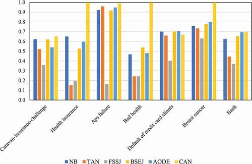
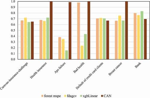
In this section, the performance of the proposed CAN method is evaluated and compared to the ones of the other Bayesian networks including NB, TAN, FSSJ, BSEJ, AODE, and other classifiers including multinomial log-linear models via neural networks, decision tree, support vector machine (SVM), k-nearest neighbors (KNN), Ada-Boost (decision tree as a base model), bagging (decision tree as a base model), extra trees, random forest mean squared prediction errors (forest MSPE) (Lu and Hardin 2019), Bagged FDA using gCV Pruning (fdagcv) (Milborrow 2019), and eXtreme Gradient Boosting (xgbLinear) (Carmona, Climent, and Momparler 2019) algorithm. These methods are applied to seven datasets described in the previous sections, based on which their performances are presented in Figures 7–9.

Figure 7. The performance (response rate) of the CAN method compared to the ones of well-known Bayesian networks.

It should be noted that the R3.4.0 software has been used in this paper to implement the proposed algorithm and to compare its performance with the ones of the competing methods. Furthermore, a computer system with an Intel Core i7-4700MQ processor and a 6- GB RAM has been employed to run the software and obtain the results.

In this paper, several R libraries including “bnclassify” (Mihaljevic, Bielza, and Larranaga 2018), “nnet” (Ripley, Venables, and Ripley 2016), “rpart” (Therneau et al. 2015), ”e1071” (Dimitriadou et al. 2008), “class” (Ripley and Venables, 2015), “adabag” (Alfaro, Gamez, and Garcia 2013), “randomForest” (Liaw and Wiener 2002), “earth” (Milborrow 2019), “caret” (Kuhn et al. 2020), “forestError” (Lu and Hardin 2019) and “xgboost” (Lu and Hardin 2019) are used to implement the proposed algorithm and the competing methods on the datasets. Moreover, the best values of the parameter $\mathrm{P}$ in Equation (15)(15) $\mathrm{S}\mathrm{p}\mathrm{e}\mathrm{a}\mathrm{r}\mathrm{m}\mathrm{a}\mathrm{n}cor\left(a_k,a_j\right)\ge \mathrm{P}$(15) , which resulted in the proposed method’s best performance when applied to different datasets, are reported in Table 3. Note that some R libraries such as “e1071” and “caret” are used for optimizing the parameters of the proposed and the competing methods where, for example, “e1071:tune.svm” function is used to select the best values of the parameters of SVM model.

Table 3. The best value of parameter $P$ for different datasets

Dataset	The best value of $\mathbf{P}$
Caravan-insurance-challenge	0.50
Health insurance	0.90
Aps failure	0.55
Bad health	0.55
Default of credit card clients	0.05
Breast cancer	0.25
Bank	0.98

Experimental Results

The results in Figures 7–9 show that the CAN algorithm performs substantially better than the competing methods in most of the datasets, resulting in the maximum performance in four cases. However, some of the other competing methods perform better than CAN when “Caravan-insurance-challenge,” “Default of credit card clients,” and “Bank” datasets are used. Nevertheless, it should be noted that in these three datasets, the performance of the CAN method is very close to the performance of the best method. Based on the results, the CAN algorithm outperformed the Bayesian networks (NB, TAN, FSSJ, BSEJ, and AODE) in six out of seven datasets. The AODE provided better performance in the case of “Default of credit card clients” while the performance of the CAN method is close to the performance of AODE. Figure 8 shows that CAN provides the best performance in five out of seven datasets compared to the seven well-known classifiers (multinomial log-linear models via neural networks, decision tree, SVM, KNN, Ada-Boost, bagging, and extra trees). Finally, the results in Figure 9 show the better performance of CAN compared to three novel algorithms (forest MSPE, Bagged FDA using gCV Pruning and eXtreme Gradient Boosting) in four out of seven datasets. Again, the performance of CAN is close to the performance of the best method in other datasets. Accordingly, one can apply the CAN method to select the customers who buy a target product more probable, correctly, and without the existing difficulties of the other complex methods.

Figure 8. The performance (response rate) of the CAN method compared to the ones of other well-known competing classifiers.

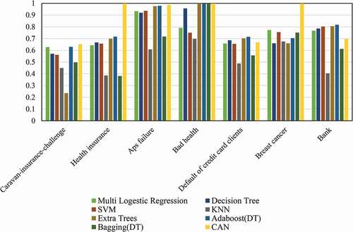
Figure 9. The performance (response rate) of the CAN method compared to novel classifiers.

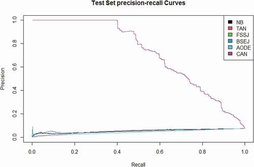
Besides, the ROC and precision-recall curves are demonstrated in Figures 10–15. These curves are obtained based on the criteria given in Equations (20)(20) $Precision=\frac{TP}{TP+FP}$(20) -(23(23) $FalsePositiveRate\left(FPR\right)=\frac{FP}{TN+FP}$(23) ).

(20) $Precision=\frac{TP}{TP+FP}$(20)

(21) $Recall=\frac{TP}{TP+FN}$(21)

(22) $TruePositiveRate\left(TPR\right)=\frac{TP}{TP+FN}$(22)

(23) $FalsePositiveRate\left(FPR\right)=\frac{FP}{TN+FP}$(23)

Figure 10. The ROC curves of forest MSPE, Bagged FDA using gCV Pruning and eXtreme Gradient Boosting compared to the CAN algorithm for the “health insurance” data set.

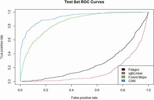
Figure 11. The Precision-Recall curves of forest MSPE, Bagged FDA using gCV Pruning and eXtreme Gradient Boosting compared to the CAN algorithm for the “health insurance” data set.

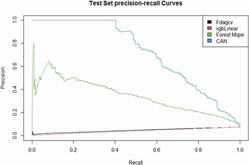
Figure 12. The ROC curves of the multinomial log-linear model via the neural network, decision tree, SVM, KNN, Ada-Boost, bagging, and extra trees compared to the CAN algorithm for the “health insurance” data set.

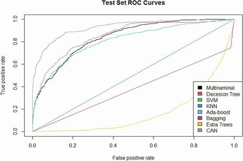
Figure 13. The Precision-Recall curves of the multinomial log-linear model via the neural network, decision tree, SVM, KNN, Ada-Boost, bagging, and extra trees compared to the CAN algorithm for the “health insurance” data set.

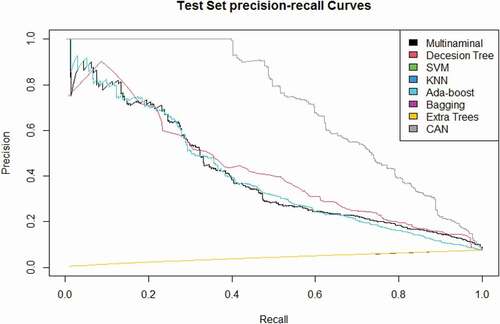
Figure 14. The ROC curves of NB, TAN, FSSJ, BSEJ, and AODE compared to the CAN algorithm for the “health insurance” data set.

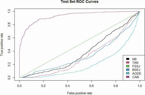
Figure 15. The Precision-Recall curves of NB, TAN, FSSJ, BSEJ, and AODE compared to the CAN algorithm for the “health insurance” data set.

in which $TN$ (true negative), $TP$ (true positive), $FP$ (false positive), and $FN$ (false negative) are defined in the confusion matrix given in Table 4.

Table 4. The confusion matrix of binary classification

	Predicted Zero Class	Predicted One Class
Actual Zero Class	$TN$	$FP$
Actual One Class	$FN$	$TP$

The curves given in Figures 10–15 compare the performance of the CAN algorithm with the competing methods where they indicate that CAN performs remarkably better than the competing methods under different thresholds and it is the best method at most of the thresholds. The ROC and precision-recall curves are only presented for the “health insurance” data set to save spaces, while the same conclusions can be obtained for other datasets.

In summary, the proposed CAN algorithm performs better than the competing methods for datasets with different characteristics in most cases. The proposed algorithm performs well under different conditions, including imbalanced datasets, missing data, the presence of different types of variables such as nominal variables, and various applications. It should be noted that if a dataset has nominal variables, they should be changed to rank variables in the CAN algorithm.

Concluding Remarks

In this paper, an improved version of the naïve Bayesian (NB) classifier called correlation-augment naïve Bayes (CAN) was proposed as a Bayesian method. It relaxes the assumption of using independent attributes embedded in the NB classifier and works well under imbalanced datasets. At the same time, it retains the simplicity of the Bayesian classifier. The performance of the CAN method was evaluated and compared with several well-known Bayesian networks and other sophisticated classifiers in terms of the response rate for which all methods were applied on seven different datasets with different application areas and different characteristics. The results showed that the proposed CAN method performs significantly better than the competing methods in almost all of the scenarios under different application areas, different number of attributes, different number of samples, imbalanced datasets, and in the presence of missing data.

Extending the proposed approach for situations where there are more than two possible values for the class-label attribute is an interesting subject that is recommended for future research. In addition, investigating different topologies of Bayesian networks to improve the performance and, at the same time, retain the simplicity of the method is recommended for future research.

Disclosure statement

No potential conflict of interest was reported by the author(s).

Additional information

Funding

This research did not receive any specific grant from funding agencies in the public, commercial, or not-for-profit sectors.

Notes

1. https://drive.google.com/file/d/1XhjAvHQDK1vI4VeorXNqyxGMD6xz_4EB/view?usp = sharing

References

- Alfaro, E., M. Gamez, and N. Garcia. 2013. Adabag: an R package for classification with boosting and bagging. Journal of Statistical Software 54 (2):1–35. doi:https://doi.org/10.18637/jss.v054.i02.
- Ansari, A., C. F. Mela, and S. A. Neslin. 2008. Customer channel migration. Journal of Marketing Research 45 (1):60–76. doi:https://doi.org/10.1509/jmkr.45.1.60.
- Baesens, B., S. Viaene, D. Van Den Poel, J. Vanthienen, and G. Dedene. 2002. Bayesian neural network learning for repeat purchase modelling in direct marketing. European Journal of Operational Research 138 (1):191–211. doi:https://doi.org/10.1016/S0377-2217(01)00129-1.
- Beheshtian-Ardakani, A., M. Fathian, and M. Gholamian. 2018. A novel model for product bundling and direct marketing in e-commerce based on market segmentation. Decision Science Letters 7 (1):39–54. doi:https://doi.org/10.5267/j.dsl.2017.4.005.
- Blanco, R., I. Inza, M. Merino, J. Quiroga, and P. Larrañaga. 2005. Feature selection in Bayesian classifiers for the prognosis of survival of cirrhotic patients treated with TIPS. Journal of Biomedical Informatics 38 (5):376–88. doi:https://doi.org/10.1016/j.jbi.2005.05.004.
- Burton, S. H., R. G. Morris, C. G. Giraud-Carrier, J. H. West, and R. Thackeray. 2014. Mining useful association rules from questionnaire data. Intelligent Data Analysis 18 (3):479–94. doi:https://doi.org/10.3233/IDA-140652.
- Carmona, P., F. Climent, and A. Momparler. 2019. Predicting failure in the US banking sector: an extreme gradient boosting approach. International Review of Economics & Finance 61:304–23. doi:https://doi.org/10.1016/j.iref.2018.03.008.
- Chen, D., S. L. Sain, and K. Guo. 2012. Data mining for the online retail industry: A case study of RFM model-based customer segmentation using data mining. Journal of Database Marketing & Customer Strategy Management 19 (3):197–208. doi:https://doi.org/10.1057/dbm.2012.17.
- Chen, Z.-Y., Z.-P. Fan, and M. Sun. 2015. Behavior-aware user response modeling in social media: Learning from diverse heterogeneous data. European Journal of Operational Research 241 (2):422–34. doi:https://doi.org/10.1016/j.ejor.2014.09.008.
- Chow, C., and C. Liu. 1968. Approximating discrete probability distributions with dependence trees. IEEE Transactions on Information Theory 14 (3):462–67. doi:https://doi.org/10.1109/TIT.1968.1054142.
- Coussement, K., P. Harrigan, and D. F. Benoit. 2015. Improving direct mail targeting through customer response modeling. Expert Systems With Applications 42 (22):8403–12. doi:https://doi.org/10.1016/j.eswa.2015.06.054.
- Darzi, M. R. K., S. T. A. Niaki, and M. Khedmati. 2019. Binary classification of imbalanced datasets: The case of COIL Challenge 2000. Expert Systems with Applications 128:169–86. doi:https://doi.org/10.1016/j.eswa.2019.03.024.
- De Campos, C. P., G. Corani, M. Scanagatta, M. Cuccu, and M. Zaffalon. 2016. Learning extended tree augmented naive structures. International Journal of Approximate Reasoning 68:153–63. doi:https://doi.org/10.1016/j.ijar.2015.04.006.
- Dheeru, D., and E. K. Taniskidou (2017). “UCI machine learning repository.” University of California, Irvine, School of Information and Computer Sciences. https://archive.ics.uci.edu/ml
- Dimitriadou, E., K. Hornik, F. Leisch, D. Meyer, and A. Weingessel. 2008. Misc functions of the department of statistics (e1071), TU Wien. R Package 1:5–24.
- Dutta, S., S. Bhattacharya, and K. K. Guin (2015). Data mining in market segmentation: A literature review and suggestions. Proceedings of Fourth International Conference on Soft Computing for Problem Solving, Springer, New Delhi, pp: 87–98.
- Elsalamony, H. A. 2014. Bank direct marketing analysis of data mining techniques. International Journal of Computer Applications 85 (7):12–22. doi:https://doi.org/10.5120/14852-3218.
- Elsalamony, H. A., and A. M. Elsayad. 2013. Bank direct marketing based on neural network and C5. 0 models. International Journal of Engineering and Advanced Technology (IJEAT) 2 (6):392–400.
- Friedman, N., D. Geiger, and M. Goldszmidt. 1997. Bayesian network classifiers. Machine Learning 29 (2/3):131–63. doi:https://doi.org/10.1023/A:1007465528199.
- Greene, W. 2008. Functional forms for the negative binomial model for count data. Economics Letters 99 (3):585–90. doi:https://doi.org/10.1016/j.econlet.2007.10.015.
- Han, J., J. Pei, and M. Kamber. 2011. Data mining: Concepts and techniques. Elsevier, MA, USA.
- Koumétio, C. S. T., W. Cherif, and S. Hassan (2018). Optimizing the prediction of telemarketing target calls by a classification technique. 2018 6th International Conference on Wireless Networks and Mobile Communications (WINCOM), IEEE, Marrakesh, Morocco.
- Koumétio, S. C. T., and H. Toulni. 2021. Improving KNN Model for Direct Marketing Prediction in Smart Cities. In: Ghosh U., Maleh Y., Alazab M., Pathan AS.K. (eds) Machine Intelligence and Data Analytics for Sustainable Future Smart Cities. Studies in Computational Intelligence, vol 971. Springer, Cham. https://doi.org/https://doi.org/10.1007/978-3-030-72065-0_7
- Kuhn, M., J. Wing, S. Weston, A. Williams, C. Keefer, A. Engelhardt, T. Cooper, Z. Mayer, B. Kenkel, R. C. Team, M. Benesty, R. Lescarbeau, A. Ziem, L. Scrucca, Y. Tang, C. Candan, and T. Hunt. 2020. Caret: Classification and Regression Training. R Package Version 6.0–90. https://CRAN.r-project.org/package=caret
- Lawi, A., A. A. Velayaty, and Z. Zainuddin (2017). On identifying potential direct marketing consumers using adaptive boosted support vector machine. Computer Applications and Information Processing Technology (CAIPT), 2017 4th International Conference on, IEEE, Kuta Bali, Indonesia.
- Liaw, A., and M. Wiener. 2002. Classification and regression by randomForest. R News 2 (3):18–22.
- Ling, C. X., and C. Li. 1998. Data mining for direct marketing: Problems and solutions. KDD 98:73–79.
- Lu, B., and J. Hardin (2019). “A unified framework for random forest prediction error estimation.” arXiv preprint arXiv:1912.07435.
- Miguéis, V. L., A. S. Camanho, and J. Borges. 2017. Predicting direct marketing response in banking: Comparison of class imbalance methods. Service Business 11 (4):831–49. doi:https://doi.org/10.1007/s11628-016-0332-3.
- Mihaljevic, B., C. Bielza, and P. Larranaga (2018). “Technical details for the bnclassify package.”http://cran.nexr.com/web/packages/bnclassify/vignettes/technical.pdf.
- Mihaljević, B., C. Bielza, and P. Larrañaga. 2018. bnclassify: learning Bayesian network classifiers. The R Journal 10 (2):455–68. doi:https://doi.org/10.32614/RJ-2018-073.
- Milborrow, M. S. (2019). “Package ‘earth.’” R Software package.
- Mitik, M., O. Korkmaz, P. Karagoz, I. H. Toroslu, and F. Yucel. 2017. Data mining approach for direct marketing of banking products with profit/cost analysis. The Review of Socionetwork Strategies 11 (1):17–31. doi:https://doi.org/10.1007/s12626-017-0002-5.
- Moro, S., P. Cortez, and P. Rita. 2014. A data-driven approach to predict the success of bank telemarketing. Decision Support Systems 62:22–31. doi:https://doi.org/10.1016/j.dss.2014.03.001.
- Moro, S., R. Laureano, and P. Cortez (2011). Using data mining for bank direct marketing: An application of the crisp-dm methodology. Proceedings of European Simulation and Modelling Conference-ESM’2011, EUROSIS-ETI, Guimaraes, Portugal, pp: 117–21.
- Nachev, A., and M. Hogan (2014). Application of multilayer perceptrons for response modeling. Proceedings on the International Conference on Artificial Intelligence (ICAI), The Steering Committee of The World Congress in Computer Science, Computer Engineering and Applied Computing (WorldComp), Las Vegas, USA.
- Olson, C. A. 1998. A comparison of parametric and semiparametric estimates of the effect of spousal health insurance coverage on weekly hours worked by wives. Journal of Applied Econometrics 13 (5):543–65. doi:https://doi.org/10.1002/(SICI)1099-1255(1998090)13:5<543::AID-JAE507>3.0.CO;2-J.
- Ou, C., C. Liu, J. Huang, and N. Zhong. 2003. On data mining for direct marketing. In International Workshop on Rough Sets, Fuzzy Sets, Data Mining, and Granular-Soft Computing, 491-498. Springer, Berlin, Heidelberg.
- Parlar, T., and S. K. Acaravci. 2017. Using data mining techniques for detecting the important features of the bank direct marketing data. International Journal of Economics and Financial Issues 7 (2):692–96.
- Pazzani, M. J. 1996. Searching for dependencies in Bayesian classifiers. In Learning from Data, 239-248. Springer, New York, NY.
- Ratanamahatana, C. A., and D. Gunopulos (2002). “Scaling up the naive Bayesian classifier: using decision trees for feature selection.” In Proceedings of the IEEE International Conference on Data Mining (ICDM 2002), Maebashi, Japan, pp: 475–87
- Ripley, B., and W. Venables “class: functions for classification, 2015.” R package version: 7.3–14.
- Ripley, B., W. Venables, and M. B. Ripley. 2016. Package ‘nnet.’ R Package Version 7:3–12.
- Seret, A., A. Bejinaru, and B. Baesens. 2015. Domain knowledge based segmentation of online banking customers. Intelligent Data Analysis 19 (s1):S163–S184. doi:https://doi.org/10.3233/IDA-150776.
- Sun, B., S. Li, and C. Zhou. 2006. ““Adaptive” learning and “proactive” customer relationship management. Journal of Interactive Marketing 20 (3–4):82–96. doi:https://doi.org/10.1002/dir.20069.
- Tavana, M., A. R. Abtahi, D. Di Caprio, and M. Poortarigh. 2018. An artificial neural network and Bayesian network model for liquidity risk assessment in banking. Neurocomputing 275:2525–54. doi:https://doi.org/10.1016/j.neucom.2017.11.034.
- Therneau, T., B. Atkinson, B. Ripley, and M. B. Ripley (2015). Package ‘rpart.’ Available online: cran.ma.ic.ac.uk/web/packages/rpart/rpart.pdf (accessed on 20 April 2016).
- Van Der Putten, P., and M. Van Someren (2000). “CoIL challenge 2000: The insurance company case.” Published by Sentient Machine Research, Amsterdam. Also a Leiden Institute of Advanced Computer Science Technical Report 9: 1–43.
- Verhoef, P. C., P. N. Spring, J. C. Hoekstra, and P. S. Leeflang. 2003. The commercial use of segmentation and predictive modeling techniques for database marketing in the Netherlands. Decision Support Systems 34 (4):471–81. doi:https://doi.org/10.1016/S0167-9236(02)00069-6.
- Vriens, M., H. R. Van Der Scheer, J. C. Hoekstra, and J. Roelf Bult. 1998. Conjoint experiments for direct mail response optimization. European Journal of Marketing 32 (3/4):323–39. doi:https://doi.org/10.1108/03090569810204625.
- Webb, G. I., J. R. Boughton, and Z. Wang. 2005. Not so naive Bayes: Aggregating one-dependence estimators. Machine Learning 58 (1):5–24. doi:https://doi.org/10.1007/s10994-005-4258-6.
- Wissler, C. 1905. The Spearman correlation formula. Science 22 (558):309–11. doi:https://doi.org/10.1126/science.22.558.309.
- Yeh, I.-C., C.-H. Lien, T.-M. Ting, and C.-H. Liu. 2009. Applications of web mining for marketing of online bookstores. Expert Systems with Applications 36 (8):11249–56. doi:https://doi.org/10.1016/j.eswa.2009.02.068.
- Zakaryazad, A., and E. Duman. 2016. A profit-driven Artificial Neural Network (ANN) with applications to fraud detection and direct marketing. Neurocomputing 175:121–31. doi:https://doi.org/10.1016/j.neucom.2015.10.042.