A New Approach for Predicting the Future Position of a Moving Object: Hurricanes’ Case Study

ABSTRACT

Currently, huge amount of data, resulting from the continuous tracking of moving objects, are collected, and stored in appropriate repositories. From these data trajectory data are generated and analyzed to produce knowledge useful for decision-making. Obviously, trajectory data sets need efficient and effective analysis and mining processes to infer mobility patterns and consequently constitute rich sources for many contributions such those related to predictions. Most of researches, presented in the literature, focus on tracking and predicting moving object positions, without taking into account their ever-changing contexts and their environmental impacts. Any environment surrounding any object is dynamic vs static and its influence goes beyond current state to the predicted ones. The aim of this paper is not only to propose a new approach to predict the future position of a moving object based on mobility patterns but also it takes into account the ever-evolving contexts and environments of the underlying objects. We experimented our approach on real case study datasets related to hurricanes’ activities. The proposed approach is performed in three phases. The first phase allows the generation of object mobility patterns. In the second phase, spatiotemporal mobility rules are extracted from the previously generated patterns. In the third and last phase, hurricane future position prediction is accomplished by using the extracted rules enhanced by context and environmental characteristics. The proposed model leads to a generic one representing facts and discovering knowledge through various applications including different mobile objects and their associated patterns, environmental and contexts.

Introduction

During the recent years, information resulting from moving objects has attracted great interest by data scientists, both in industrial and academic fields. This information is called trajectory data since it describes and contains information about moving objects trajectories (Oueslati and Akaichi 2010) and constitutes a rich source for inferring mobility patterns. Such information is used to extract useful knowledge about what, how and for how long the moving entities are conducting individual activities related to specific circumstances. Therefore, mining moving object trajectory data is needed. One of the important mining processes available for moving objects is the prediction process, because it allows having idea about the possible future locations of moving objects. Broadly moving objects are geometries (points, lines, regions) changing positions over time (Güting and Schneider 2005). A point represents the geometrical aspect of an object. Examples of point objects are area unit cities on an oversize scale map, landmarks, hospitals, or subway stations. A line (in this context invariably means a curve in space) is the basic abstraction for moving through space, or connections in area. Finally, a region is the abstraction for an entity having an extent in the 2D space. A region may consist of holes and several disjoint pieces; for example, countries, forests, hurricanes or lakes are the main region objects. Many research works focus on future position prediction of moving objects as moving point (Wiest et al. 2012, Qiao et al. 2015, Monreale et al. 2009, Ying, Lee, and Tseng 2013) and much less on moving objects as moving region (Hoang, Zheng, and Singh 2016, Ziliani and Surian 2016, Castelli, Vanneschi, and Popovič 2015) future position. In fact, few works were interested in the analysis and the prediction of moving regions’ future locations depending on the history of their trajectory data. Predicting moving regions’ future position plays an important role in applications that deal with monitoring and tracking environmental events as well as natural phenomena. For this reason, we propose in this work a spatiotemporal mobility prediction pattern–based approach. The proposed approach leads to the prediction of the future location of a moving region (hurricane) traveling in space during a time interval. The novelty and the main contributions of this work are as follows: (1) Dealing with hurricanes as moving regions that have spatiotemporal and semantic aspects. Those latter constitute hurricanes’ trajectory data that will be exploited as inputs in the knowledge discovery process. (2) Exploratory data visualization of hurricanes is being carried out. (3) The development of improved data mining approach for predicting the possible future position of hurricanes based on spatiotemporal variables along with meteorological variables such as wind-speed, gust-speed, central pressure and so on. The rest of this paper is organized as follows: The second section focuses on different approaches that lead to predicting future position of moving objects. The third section describes in details the different phases of the proposed approach. In the fourth section, we validate the works. Finallys, the last section concludes our work and gives future directions of our research Figure 1.

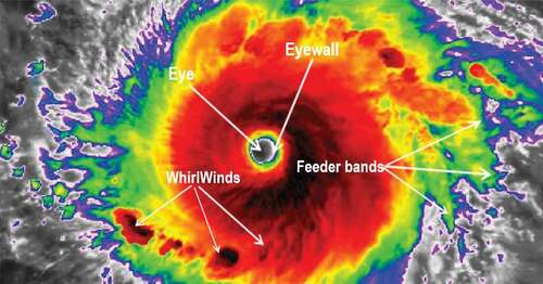
Figure 1. Hurricane structure by NOAA Center (https://www.nhc.noaa.gov).

Previous Work

In this section, we present the different existing approaches that deal with moving objects’ future position prediction.

Scientists are interested in improving the ability of predictive models to track moving objects’ future trajectories. Various forecast prediction models that generate knowledge about the mobile objects’ future positions are proposed in the literature. We divided the prediction studies into two categories: the frequent pattern mining-based methods and the machine learning-based methods.

The Frequent Pattern Mining-Based Prediction Methods

Depending on the priori knowledge mining from historical trajectories to predict future locations, the decision tree is considered the most common method. Monreale in Monreale et al. (2009) has proposed a prefix tree called the ‘T-pattern tree.’ The approach, uses the trajectory patterns as a predictor of the next location of a new trajectory and then find the best matching path in the tree. The evaluation function took into consideration three aspects: the spatial coverage, the data set coverage and the spatial separation. Ying, Lee, and Tseng (2013) proposed a novel mining-based location prediction approach called Geographic-Temporal-Semantic-based Location Prediction (GTS-LP), which took into account a user’s geographic, temporal and semantic-triggered intentions to estimate the probability of the user in visiting a location. The core idea underlying the proposed approach is the discovery of trajectory patterns of users, namely GTS Patterns, to capture frequent movements triggered by the three kinds of intentions. The Bikely allows users to upload GPS logs within a trip and tag a trip using semantic terms. The main measurements applied in the experimental evaluation are the precision, coverage, F-measure and average. Yavaş et al. (2005) have proposed an algorithm for predicting the next inter-cell movement of a mobile user in a Personal Communication System network. They addressed the problem of mining offline mobility data from mobile user trajectories to discover regularities in inter-cell movements called mobility patterns and extract mobility rules from these patterns. The mobility rules, which match the current trajectory of a mobile user, are used for the online prediction of the user’s next movement. In their experimental study, the proposed approach has reached high precision and recall.

Yang and Hu (2006) have proposed a model for trajectory patterns and a new measure to represent the importance of a trajectory pattern and to estimate the expected occurrences of a pattern in a set of imprecise trajectories. In particular, they defined a new property, called min-max, where they devise the so-called TrajPattern algorithm. This latter mines k trajectory patterns by a growing process. The first step is to identify short patterns that have the highest normalized match measure. The second step is to extend the resulting short patterns from the previous step in order to find longer patterns via the min-max property with high normalized measure. Due to the presence of noise in the trajectories, many similar patterns may be found in the mining process. For this reason, the concept of pattern groups was proposed.

Ayat, Evans, and Behrangi (2021) studied the effect of different sources of data in the uncertainties of a merged multi-satellite retrieval product during the hurricane events (2016–2018) using both pixel-based and object-based approach. For this purpose, they compare the multi-satellite retrieval product with a ground-based radar product. The results showed that merged product has better agreement in terms of the average precipitation intensity and area when the passive microwave (PMW) sensor overpass is matched instantaneously with the radar product compared to temporally averaged radar data. PMW observations tend to show storms with smaller areas in the satellite-based product in comparison with the radar one, possibly because of light precipitation not detected properly by PMW sensors. However, by removing the light precipitation (less than 1 mm/h) in the object-based approach, hurricane objects in the satellite-based product tend to be larger during the PMW observations, which might be related to different viewing angles of sensors contributing to satellite and radar products.

Machine Learning–Based Prediction Methods

Prediction methods based on machine learning are used to improve the models by exploring the behavioral characteristics of moving objects from their historical trajectories in order to realize trajectory prediction using trained models such as the Markov model (a stochastic model used to model randomly changing systems), probabilistic graphical model, network model, etc. Many machine learning–based approaches are proposed in the literature to tackle the problem of predicting natural disasters such as cyclones, typhoons and hurricanes.

Camargo et al. (2007) proposed a probabilistic clustering technique, based on a regression mixture model to describe tropical cyclone trajectories in the western North Pacific. Each component of the mixture model consists of a quadratic regression curve of cyclone position against time. The best-track 1950–2002 data set is described by seven distinct clusters. These clusters are then analyzed in terms of genesis location, trajectory, landfall, intensity, and seasonality. Several distinct types of straight-moving, as well as recurving, trajectories are identified. Intensity and seasonality of cyclones, though not used by the clustering algorithm, are both highly stratified from cluster to cluster. Three straight-moving trajectory types have very small within cluster spread, while the recurving types are more diffuse. Tropical cyclone landfalls over East and Southeast Asia are found to be strongly cluster dependent, both in terms of frequency and region of impact. Qiao et al. (2015) propose a trajectory prediction algorithm based on the self-adaptive parameter-selection hidden Markov model.

Chen, Yu, and Liu (2016) proposed a weighted Markov model (weighted-MM) to consider both the sequence of just-passed locations and object similarity for mining mobility patterns. They tested a Markov model for each object with its own trajectory records, and so quantified the similarities between totally different objects from two aspects that are the spatial neighborhood similarity and the trajectory similarities. Finally, they incorporated the object similarity into the Markov model by taking into consideration the weight of the probability of reaching each possible next position as a similarity factor, and then return the top-rankings as results.

Goerss, Sampson, and Gross (2004) proposed a tropical cyclone (TC) track forecasting skill of operational numerical weather prediction (NWP) models and their consensus is examined for the western North Pacific from 1992 to 2002. While the addition of models to the consensus has a modest impact on forecast skill, it has a more marked impact on consensus forecast availability. The forecast availabilities for 72-h consensus forecasts computed from a pool of two, five, seven, and eight models were 84, 89, 92, and 97%, respectively. Ishikawa, Tsukamoto, and Kitagawa (2004) proposed an approach that extracts mobility statistics from indexed spatiotemporal data sets for interactive analysis of enormous sets of moving object trajectories. They focused on mobility statistics calling the Markov transition probability, which is based on a cell-based organization of a target space and the Markov chain model. The proposed approach of Ishikawa, Tsukamoto, and Kitagawa (2004) structures the trajectories in an R-tree index and computes mobility statistics, termed as Markov transition probabilities, by using the index. The transition possibilities enable to calculate future cells by victimization state information from the present cells. The proposed algorithm reduces the mobility statistics computation task to a constraint satisfaction problem. Using such statistical mobility information, researchers can estimate if an object at some region at instant T will move to another region in the next period with a high probability. It assigns the cells expressing the spatial constraints to enumerated teams of objects that satisfy a sort of temporal constraints. The constraint satisfaction problem (CSP) is solved from the foundation toward the leaves of the index outlined by the spatiotemporal constraints. Alemany et al. (2018a) proposed a fully connected recurrent neural network (RNN). Those latter are nonlinear dynamical models that are commonly used in machine learning to represent complex dynamical or sequential relationships between variables (McDermott and Wikle 2019). They allow predicting the trajectory of hurricane in order to have an idea about the hurricane’s behavior. A grid system was used with the intention to encapsulate the non linearity and complexity behind forecasting hurricane trajectories and potentially increasing the accuracy compared to operating hurricane track forecasting model. The raw Atlantic hurricane data applied in this study (Alemany et al. 2018a) were taken from the NOAA database. The data include all hurricanes and tropical storms from 1920 to 2012. They utilized Keras for the implementation, which is an API that combine lower-level deep learning languages such as TensorFlow. The proposed model predicts the next hurricane location at 6 hours, as well it has the ability to pack up the historical information about the nonlinear dynamics of the atmospheric system by upgrading the weight matrices appropriately. This capability makes the RNN suitable for modeling the complex system of hurricane behavior with unobservable states. Recently, Zhao et al. (2018) applied a deep bidirectional long short-term memory (BLSTM) and mixture density network (MDN) approach (BLSTM-MDN). The LSTM control what needs to be preserved and what needs to be forgotten. That’s why LSTM can retain information from a long time ago. BLSTM is derived from LSTM. Its main plan is that the output of every layer can process information from both forward units and backward units. This model is not only capable of predicting a basketball trajectory based on real data, but it also can generate new trajectory samples to predict basketball trajectories. Alemany et al. (2018b) proposed a new approach with recurrent neural network (RNN) to predict the trajectory of hurricanes based on their latitude, longitude, wind speed and pressure. The RNN learn the behavior of a hurricane trajectory from a grid model to reduce the number of truncation errors due to computational limitations. According to the experimentation, the proposed approach can approximately predict 120 hours of the hurricane path.It is considered as the first fully connected recurrent neural networks used with a grid model to predict hurricanes trajectories accurately. Kowaleski and Evans (2020) applied a multi-ensemble model track clustering to generate deterministic forecasts of tropical cyclone position and intensity. Clustering was performed on four data sets. Each one has five cluster partitions. Authors used the pruning methods. Ensemble-mean forecast error before and after pruning are compared and results show that pruning methods reduce ensemble-mean forecast errors.

Running Example: Hurricane from Meteorology Perspective

Scientific and technological advances in recent decades have greatly improved the nation’s capability to predict most natural disasters and disseminate warnings based on those predictions (Council et al. 1991). Disasters may be explosions, earthquakes, floods, hurricanes, tornados, or fires. Disasters inflict serious damage and so seem to be bad for the economy what lead to destruction of property and loss of financial resources (Raschky 2008). For firms, natural disasters destroy tangible assets such as buildings and equipment as well as human capital and thereby deteriorate their production capacity. In our work, the moving region is a natural disaster that is the hurricane, it is a powerful meteorological depression that forms in the tropics and the engine is an atmospheric convection with the meeting of different other factors such as warm sea surface temperature that must be above 26°C, low vertical wind shear especially in the upper level of the atmosphere, the high relative humidity values from the surface to the wind levels of the atmosphere, the saturated lapse rate gradient near the center of rotation of the storm and the spin of the earth. Hurricanes are considered as the major natural disasters that lead to destruction and loss of lives. To reduce this harm caused by this kind of natural disaster, the most prevention measure is to predict their future locations. Researchers have become interested in improving the capability of predictive models for tracking hurricanes trajectories (Hall and Jewson 2007). Therefore, they developed over the years some diagnostic techniques to predict their movements in order to reduce human and economic losses. Hurricane forecasting was firstly tackled from a meteorological perspective. According to Willoughby, Rappaport, and Marks (2005), hurricanes are circular cyclonic storms that draw their energy from the warm tropical sea. They are distinct from middle-latitude cyclones which depend on the tropics-to-pole horizontal temperature gradient for their energy. Hurricanes are 500–1,000 km in horizontal extent, much smaller than middle latitude cyclones. Hurricanes are warm core in the sense that the air near the center is warmer than the surrounding atmosphere. Because warm air is less dense than cold, this property causes their low hydrostatic central pressures, which can be as much as 10% below that in the normal tropical atmosphere. In the past a forecast was considered successful if it specified the position and intensity of the hurricane for times ranging from 24 through 72 hours after the initial time. By the 1990s, users came to expect a great deal of specific detail, including spatial distributions of rainfall, winds, flooding and high seas, for times as long as 120 hours into the future. Meteorologists have maintained reliable, homogenous statistics on forecast accuracy for more than a half-century. These “verification” statistics provide reliable metrics of meteorological performance. Because hurricanes are compact, long-lived weather systems, forecasts of their positions and intensities – measured in terms of maximum wind – are the first steps toward characterizing the threat. Marks et al. (1998) present an authoritative, though now somewhat dated, plan for hurricane forecasting and related research. The highest priority has historically been predicting the cyclones’ future paths, which is called track forecasting. The track worries everyone in the threatened area, whereas intensity is of overwhelming concern only to those directly in the cyclone’s path. Despite steadily improving accuracy, warning areas increased during the late 20th century because emergency managers wanted to ensure that nobody was struck without warning, as well as to gain more lead time for evacuating ever-increasing coastal populations. Since 2000, the size of warning areas has decreased somewhat in response to more accurate forecasts. Output from computer models, called guidance, is the primary tool for track forecasting. Statistical extrapolations based on numerical predictions of global wind and pressure patterns Numerical models are structured on a computational grid with temperature, moisture, and wind tabulated in more-or-less rectangular cells. The models calculate the spatial derivatives that appear in the equations by finite differences and extrapolate the computed time derivatives forward to predict the future weather elements on the grid. As computers become faster with larger memories, these models can use finer spatial resolution and more elaborate representation of physical processes to attain increasing accuracy. Guidance is the primary tool for track forecasting based on computer capabilities according to DeMaria and Gross (2013), statistical extrapolations based on numerical predictions of global wind and pressure patterns, once resulted in the most accurate guidance. These statistical–dynamical schemes superseded earlier are purely statistical models based on observed weather. According to Landsea and Cangialosi (2018), in spite of the improvements in forecasting tropical cyclone track, making perfect forecasts is very difficult to happen.

For a good understanding of the hurricane concepts, we present hurricane’s different components. In fact, hurricanes are considered as moving region. They are characterized by a set of attributes such as the wind-speed, the gust-speed (a sudden and strong thost of wind), the direction, the location, and the trajectory (path). The main parts of a hurricane are the feeder bands on its outer edges, the whirlwinds, the outflow, the eye and the eyewall. The eye represents the center of the storm, where the clouds clusters up like a stadium. It is the calmest part of the storm. The eye is surrounded by the eyewall, which is composed of dense clouds. This is the location within a hurricane where the most damaging winds and intense rainfall is found. Feeder Bands revolves around its main components (eye, eyewall) and spiral out of the storm, which extend outward from a hurricane’s scouter. Rainfall beneath them is torrential. Those bands are obscured by higher level clouds and whirlwinds that surround a hurricane, which is considered as one of its most crucial factors. The hurricane moved according to these winds. The prevailing winds that surround a hurricane are known as the environmental winds spiral and guide the hurricane along its path. The hurricane propagates in the direction of those whirlwinds, which also impact the hurricane’s propagation speed. Each whirlwind is developed over time with high wind speed. the natural factors help whirlwind to become more speed and every single one makes its own trajectory.

A Data Mining Approach for Location Prediction of Hurricane Future Position

In the pattern mining problem discussed in Yavaş et al. (2005), authors have proposed an algorithm for predicting the next internode movement of a mobile user in a Personal Communication Systems network. The approach is composed of three phases that are the user mobility pattern mining, the generation mobility rules and the mobility pattern. For our case study, the moving object is a moving region that is the hurricane. The approach proposed in Yavaş et al. (2005) cannot be applied directly to our case study for mining mobility patterns, because it did not take into account the temporal concept evolution. The approach followed by Yavaş et al. (2005) for mining user mobility pattern of mobile users has a completely different basis than hurricane movement. In fact, a mobile user is a point that represents the geometric aspect of an object, for which only its location in space is considered. Hurricanes represent a moving region which is the abstraction for an entity having an extent in the 2D space and take into consideration the spatial and temporal aspects.

Our proposed approach is composed of three main phases:

1. Object mobility pattern mining.

2. Generation of mobility rules using the mined object mobility patterns.

3. The moving object future position prediction.

The next trajectory of hurricane is predicted in the third phase based on the generated mobility rules in the second phase.

Each phase of our approach will be explained in detail in the next subsections.

Figure 2, Figure 3, Figure 4 represents the object’s future position prediction based on the generation of mobility rules process.

Figure 2. Future position prediction based on spatiotemporal mobility rules architecture.

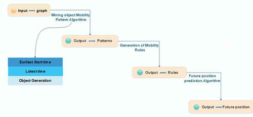
Figure 3. Whirlwind attributes according to MPM method.

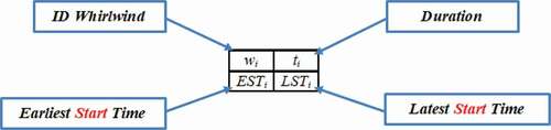
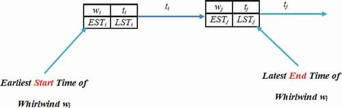
Figure 4. Clarification on MPM reading.

Mining Object Mobility Patterns from Graph Traversals

We represent an object mobility pattern as a series of neighboring positions in the coverage region network. The successive positions of an object mobility pattern ought to be neighbors on the grounds that the object cannot move among non-neighbor nodes. In reality, object mobility patterns correspond to the expected regularities of the whirlwinds absolute paths. Sequential pattern mining has been recently utilized and analyzed in different research in the literature. The most critical works are in the domain of web log mining (Nanopoulos, Katsaros, and Manolopoulos 2001, Nanopoulos, Katsaros, and Manolopoulos 2003) and mobile users’ movement behavior Yavaş et al. (2005). In Nanopoulos, Katsaros, and Manolopoulos (2001), Nanopoulos, Katsaros, and Manolopoulos (2003), sequential pattern mining is used to mine the access patterns of a user while he is visiting the pages of websites. The proposed method assumes the web pages to be the vertices and the links between these pages to be the arcs of an unweighted directed graph, G. Then, sequential pattern mining is applied to web logs by considering G. The authors generalized the same method and applied it for user mobility pattern mining and used a directed graph G, where the nodes are considered to be the vertices of G.

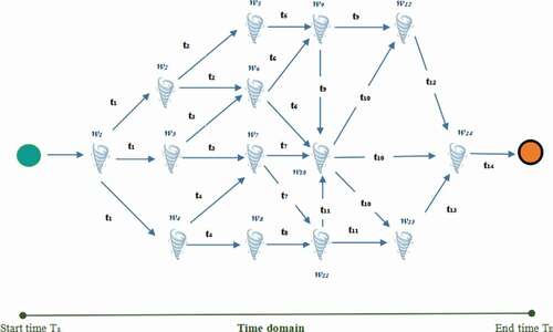
Inspired from the advantages and the popularity of the approaches presented in Nanopoulos, Katsaros, and Manolopoulos (2001), Nanopoulos, Katsaros, and Manolopoulos (2003) and Yavaş et al. (2005), we choose to propose a new method that is most suitable for our domain and employ it for hurricane future position prediction. We used a directed graph G. The graph representation can offer a more cohesive methodology for representing the different phases of a hurricane trajectory as a directed graph. We took the approach of mining our patterns during time interval [start-time, end-time] by time interval basis that consists of organizing the movement of objects over time, taking into account temporal constraints. This is important because it allows us to see the changing nature of the patterns over time and allows an interactive mining including changing the mining parameters. Even though the patterns that we consider occur in a spatial setting, they are all temporal patterns because they describe objects’ movements over time, as well as capturing changes in the way the objects move over time.

For a better understanding, we consider each pattern $W_k$ as capturing object movements over a “short” period of time. The short period time is represented as pair interval [start-time, end-time]. That is, $W_k$ contains all the spatiotemporal mobility aspect, stationary regions during [start-time, end-time], and as such captures how the objects move between the time intervals [start-time, end-time].

Then, as the algorithm processes subsequent time intervals, the patterns mined will in general change, forming a sequence of pattern sets $w_1,w_2,\dots .$ Any significant change in the patterns can be considered longer term change. Such changes affect the objects’ behavior over time. Another way to think about this is to consider the objects’ motion as a random process. If the process is stationary, we would expect that the patterns remain roughly the same over time. If the process is not stationary, the patterns will change over time to reflect the change of the way the object move. On this time domain, we define a dynamic set that represent whirlwinds circulation over time. The entities are connected in time with the spatial relation called ”support” exists between two neighboring whirlwinds $w_i$ and $w_j$ respectively at time $t_i$ and $t_j$ where i < j. This means that $w_i$ ”supports” $w_j$, namely, $w_j$ depends in some way on the existence of $w_i$. This relationship generic and its interpretation depends on the application domain. This fact proves that the whirlwinds continue developing and move from $w_i$ to $w_j$ directly.

To this end, we decide to implement the Metra Potential Method (MPM), to our mobility pattern mining method. MPM is a project management tool, invented in 1958 by French researcher Bernard Roy (1971). MPM is used to describe, organize and plan the several tasks constituting a project development. This management method is similar to the PERT method (Cook 1966). It consists of an oriented graph, whose summits represent tasks and the connections represent anteriority constraints. Thanks to the use of the MPM method, the start and the end time required for each activity are easily identified. A distinguishing feature of MPM is its ability to deal with uncertainty in whirlwind completion time. For each whirlwind, the model includes two estimated times.

Hence, the whirlwinds will be represented as follows.

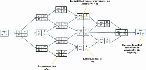
These times are calculated using the approximate time for whirlwinds. The Earliest Start Time and Latest Start Time represent whirlwind earliest and latest start times that are determined considering its predecessors whirlwinds.

The determination of Earliest Start time in order to ad it to the MPM grid consists on calculating for all whirlwinds the time at which each whirlwind begins. The initial trajectory of the hurricane starts with sprightly whirlwinds at time t = 0. Thus the value 0 is associated to the beginning node. We run the graph, node by node, from the beginning node to the ending one. Then, we calculate the time of early start of each whirlwind node.

(1) $\mathbf{E}\mathbf{a}\mathbf{r}\mathbf{l}\mathbf{i}\mathbf{e}\mathbf{s}\mathbf{t}\mathbf{S}\mathbf{t}\mathbf{a}\mathbf{r}\mathbf{t}\mathbf{T}\mathbf{i}\mathbf{m}\mathbf{e}{w}_j=\mathbf{E}\mathbf{a}\mathbf{r}\mathbf{l}\mathbf{i}\mathbf{e}\mathbf{s}\mathbf{t}\mathbf{S}\mathbf{t}\mathbf{a}\mathbf{r}\mathbf{t}\mathbf{T}\mathbf{i}\mathbf{m}\mathbf{e}{w}_i+\mathbf{D}\mathbf{u}\mathbf{r}\mathbf{a}\mathbf{t}\mathbf{i}\mathbf{o}\mathbf{n}{w}_i$(1)

When whirlwind is conditioned by more than one single antecedent whirlwind, the higher value of sum operation is kept as the earliest start time.

(2) $\mathbf{E}\mathbf{a}\mathbf{r}\mathbf{l}\mathbf{i}\mathbf{e}\mathbf{s}\mathbf{t}\mathbf{S}\mathbf{t}\mathbf{a}\mathbf{r}\mathbf{t}\mathbf{T}\mathbf{i}\mathbf{m}\mathbf{e}{w}_j=\mathbf{M}\mathbf{a}\mathbf{x}(\mathbf{E}\mathbf{a}\mathbf{r}\mathbf{l}\mathbf{i}\mathbf{e}\mathbf{s}\mathbf{t}\mathbf{S}\mathbf{t}\mathbf{a}\mathbf{r}\mathbf{t}\mathbf{T}\mathbf{i}\mathbf{m}\mathbf{e}{w}_i+\mathbf{D}\mathbf{u}\mathbf{r}\mathbf{a}\mathbf{t}\mathbf{i}\mathbf{o}\mathbf{n}{w}_i)$(2)

In the following, we present Algorithm 1 that we have proposed to get whirlwinds earliest start times:

Algorithm 1 Earliest Start Time

Input: All moving objects durations in the database $D_t$

Output: Earliest Start Time $EST$

$1:EST(0)=0$

2: read $EST(w_i)$

3: read $D_t(w_j)$ ▹ duration corresponding to object num j

4: for i = 1 to $k$ do ▹ $k$ is the last object num

5:   for j = 1 to $k$ do

6:     $EST(w_j)$= Max($EST(w_i)$+$D_t(w_i)$) ▹ maximum is computed for moving object, which is conditioned by more than one single antecedent object

7:   end for

8: end for

9: return $EST$

Determining the Latest Start time in order to add it to the MPM grid consists on calculating for all whirlwinds the time at which each whirlwind can start at latest. The Latest Start time at the end of hurricane is equal to the Earliest Start Time of hurricane. We will therefore place the Earliest Start Time in the box Latest Start Time associated with the End node. Then, we go, from the ending node up to the beginning node. The Latest Start time of each whirlwinds is thus gradually calculated as follows:

(3) $\mathbf{L}\mathbf{a}\mathbf{t}\mathbf{e}\mathbf{s}\mathbf{t}\mathbf{S}\mathbf{t}\mathbf{a}\mathbf{r}\mathbf{t}\mathbf{T}\mathbf{i}\mathbf{m}\mathbf{e}{w}_i=\mathbf{L}\mathbf{a}\mathbf{t}\mathbf{e}\mathbf{s}\mathbf{t}\mathbf{S}\mathbf{t}\mathbf{a}\mathbf{r}\mathbf{t}\mathbf{T}\mathbf{i}\mathbf{m}\mathbf{e}{w}_j-\mathbf{D}\mathbf{u}\mathbf{r}\mathbf{a}\mathbf{t}\mathbf{i}\mathbf{o}\mathbf{n}{w}_i$(3)

When several whirlwinds start from the same whirlwind, it is better to apply this formula for all whirlwinds succeeding the concerned whirlwind and to retain as Latest Start Time the minimum founded values:

(4) $\mathbf{L}\mathbf{a}\mathbf{t}\mathbf{e}\mathbf{s}\mathbf{t}\mathbf{S}\mathbf{t}\mathbf{a}\mathbf{r}\mathbf{t}\mathbf{t}\mathbf{i}\mathbf{m}\mathbf{e}{w}_i=\mathbf{M}\mathbf{i}\mathbf{n}(\mathbf{L}\mathbf{a}\mathbf{t}\mathbf{e}\mathbf{s}\mathbf{t}\mathbf{S}\mathbf{t}\mathbf{a}\mathbf{r}\mathbf{t}\mathbf{t}\mathbf{i}\mathbf{m}\mathbf{e}{w}_j-\mathbf{D}\mathbf{u}\mathbf{r}\mathbf{a}\mathbf{t}\mathbf{i}\mathbf{o}\mathbf{n}{w}_i)$(4)

In the following, we present Algorithm 2 that we have proposed to get whirlwinds latest start times.

Algorithm 2 Latest Start Time

Input: All moving objects durations in the database $D_t$

The required completion time for the last moving object $w_k,EST(w_k)$, which is itself the latest time $LST(w_k)$

Output: Latest Time $LST$

1: read $LST(w_i)$

2: read $D_t(w_j)$

3: for i = K-1 to 0 do

4:   for j = K-1 to 0 do

5:     $LST(w_j)$=Min($LST(w_i)$-$D_t(w_j)$ ▹ minimum is computed over all moving objects, i is the beginning time

6:   end for

7: end for

8: return $LST$

We note that Latest Start Time of whirlwind j represent at same time a Latest End Time LE of whirlwind i, where i and j are successive and i ¡ j as follows.

We have extracted for each whirlwind an interval time [Earliest Start time EST, Latest End time LET].

In Figure 5, we present the associated spatiotemporal graph related to the evolution of hurricane as a moving region.

Figure 5. Corresponding graph G showing the movement of a set of objects $W_k$.

After determining the earliest and the latest start times of the moving region, our approach focuses on determining the mobility patterns. We present the ObjectMobilityPattern Mining Algorithm.

Algorithm 3 ObjectMobilityPatternMining

Input: All the ObjectActualPaths and their time intervals in the database $D$

Minimum value for support $sup{p}_{min}$

Graph $G$

Output: Object mobility patterns $L$

1: $W_1$ $\leftarrow$ the pattern which have a length of one during time interval [$EST,LET$]

2: $ES{T_W}_k$ + $LE{T_W}_k$

3: $L$=$\mathrm{\varnothing }$

4: $k$=$1$

5: $L$=$\mathrm{\varnothing }$

6: while $W_k$ $\ne$ $\mathrm{\varnothing }$ do

7:   for each ObjectActualPath $a$ $\in$ $D$ do

8:     $ES{T}_{ActualPath}$ + $LE{T}_{ActualPath}$

9:     $S$=$s$ – $s$ $\in$ $W_k$ and $s$ is a subsequence of $a$ and [$ES{T_W}_k$ + $LE{T_W}_k$] $\subset$ [$ES{T}_{ActualPath}$ + $LE{T}_{ActualPath}$]

10:     for each $s$ $\in$ $S$ do

11:       $s.count$=$s.count$+$s.suppInc$

12:     end for

13:   end for

14:   $L_k$=$s$ – $s$ $\in$ $W_k$, $s.count$ $\ge$ $sup{p}_{min}$

15:   $L$=$L$ $\cup$ $L_k$

16:   $W_{k+1}$ $\leftarrow$ ObjectGeneration($l_k$, $G$),$\mathrm{\forall }$ $w$ $W_{k+1}$ $w.count$=0

17:   $k=k+1$

18: end while

19: return $L$

Table 1 explains how the Object Mobility Pattern Mining spatiotemporal algorithm works

Table 1. ObjectMobilityPatternMining spatiotemporal algorithm description

Line	Description
Line 6	The set of candidate patterns indicated by $W_k$ each including k entities is found in the (k-1)th run of the while loop and this set is not void.
Lines 7–9	$W_k$, is called length-k whirlwinds patterns. The length-k subsequences of all ObjectActualPaths and their time intervals are produced and these subsequences are used to count the supports of the length-k whirlwinds patterns.
	We suppose that we have two ObjectActualPaths during two time intervals Y = ($y_1,y_2,\dots ,y_n,[ES{T_y}_1,LE{T_y}_n]$) and Z = ($z_1,z_2,\dots ,z_m,[ES{T_z}_1,LE{T_z}_m]$). Z is a subsequence of Y, if there exists integers 1 $\le i_1$ <¡ … ¡< $i_m\le$ n such that $z_k={z_i}_k$, for all k where 1 $\le k\le$ m.
Lines 10–13	Every Whirlwinds has a count value which is incremented by ‘s.suppInc’ value. suppInc is the support counting assigned to a whirlwind pattern $w_i$ by an ObjectActualPath $w_j$ during one time interval, we calculate the support counting following two main concepts: if the pattern $w_i$ during [$ES{T_w}_i,LE{T_w}_i$] is contained by ObjectActualPath $w_j$ during [$ES{T_w}_j,LE{T_w}_j$] then, suppInc = 1/1 +$totDist$,otherwise, suppInc = 0.
Lines 14 and 15	The next step after following counting the supports of the entire whirlwinds,the whirlwinds which have a support smaller than the threshold value $sup{p}_{min}$ are wiped out.
	The rest whirlwinds are called the length-k large patterns ($L_k$). Then,$L_k$ is added to the set in which all the large patterns are declared.
Lines 16–19	Generation of length-(k + 1) object patterns, $w_{k+1}$ using the function ObjectGeneration() presented in the next section.

The $totDist$ mentioned in Table 1 can be defined as total distance traveled between strings. As an example, let us take two strings where each one defined as a sequence of characters, by applying the demonstration methods of Gusfield (1997), we can obtain the optimal alignment and sameness between these two strings.

In case of patterns, let us suppose that we have two patterns $U=(w_3,w_4,w_0,w_1,w_6,w_5,w_8)$ and $V=(w_4,w_0,w_5)$. An optimal containment alignment of ObjectActualPath U and pattern V is linked to the lower possible limit of containment alignment score of two patterns.

We obtain the minimum value of optimal containment alignment by defining as a first step the score of alignment:

If a and b are two separate characters or spaces, then d(a,b) indicates the score of alignment of the couple a and b, so the scoring function is defined as:

d(a,b) = 0 if a = b and d(a,b) = 1 otherwise.

Here is a possible alignment of two patterns U and V, the character ’-’ represents the insertion of a space between consecutive nodes.

$U=w_3,w_4,w_0,w_1,w_6,w_5,w_8$

$V=-,w_4,w_0,-,-,w_5,-$

The value of an alignment is the result of mismatches. Our scoring function in this case is 1 for each mismatch in the alignment. The value of this containment alignment in this case is 2 and consequently the $totdist$ value will be 2. Subsequently, the support result given to V by U is $suppInc=1/1+2=1/3$. There are two main steps to calculate the supports length-k objects patterns. The first step consists of inserting all the whirlwinds patterns into tree. The second step consists of scaning the database of ObjectActualPaths. One of the most important tasks in this step is to determine all possible length-k subsequences and to calculate their $totdist$ values for each ObjectActualPath U of length $n$. Once having all the possible length-k, if $n<k$ then ObjectActualPath U is overshoot. It will not be taken into account in the support counting of length-k +1. This procedure will be continued in the next phase of searching the subsequences existing in the graph and then increasing their supports by $suppInc$. This latter is calculated with $totDist$ of the precedent subsequence.

After finishing this step, the next one is to generate length-k +1 object pattern $w_{k+1}$. For this end, we propose the ObjectGeneration algorithm.

Algorithm 4 ObjectGeneration

Input: Length-k large pattern $L_k$

Output: Length-(k +1) Object patterns $L$,Objects

1: $Objects$ = $\mathrm{\varnothing }$ ▹ Initially, the objects set is empty

2: for each $L=(l_1,l_2,\dots .,l_k),L\in L_k$ do ▹ for each length-k large pattern $L$

3: ▹ Find out all the neighboring nodes of $L_k$ existing in $G$

4:   $N$=($v$ – there is an edge in $G$ such as $l_k$ $\to$ $G$)

5:   for each $v\in \mathrm{N}({\mathrm{l}}_k)$ do ▹ for each of these neighbor nodes,$v$

6: ▹ generate moving object by attaching $v$ to end of $L$

7:     $W^{\prime }$=($l_1,l_2,\dots ,l_k,v$) ▹ Add $W^{\prime }$ to the moving object set

8:     $Objects\leftarrow \mathrm{O}\mathrm{b}\mathrm{j}\mathrm{e}\mathrm{c}\mathrm{t}\mathrm{s}\cup \mathrm{W}{ }^{\mathrm{\prime }}$

9:   end for

10: end for

11: return Moving Objects

To explain the different ObjectGeneration algorithm steps, we present the following illustrative example:

We suppose that there is a pattern $W=(w_1,w_2,\dots ,w_k)$ during time interval $[E{S}_t{w}_1,L{E}_t{w}_k]$ in the $Lenght{h}_k$ large pattern $L_k$ that was gave as input in algorithm 4.

To generate the feasible objects from $W$, all the nodes in G that have an incoming edge from the node $w_k$ are allocated to a set which is denoted by N($w_k$). This is the set of all the nodes to which our object (that is the set of whirlwinds forming the hurricane) can change its location from $w_k$.

Following that, a node $v$, from N($w_k$) is connected to the end of the pattern $W$ so a possible whirlwind $W^{\prime }=(w1,w2,\dots ,wk,v)$ is generated. If all the length-k subsequence patterns of $W^{\prime }$ (which can be as paths in the corresponding network graph $G$) are elements of $L_k$, then $W^{\prime }$ is added to the length-(k +1) objects set. This process is iterative for all the nodes in the set N($w_k$).

The theoretical execution of the Object Mobility Pattern Mining spatiotemporal algorithm with ${supp}_{min}=1$ is described step by step as follows:

For each whirlwind a duration time is accorded in Table 2.

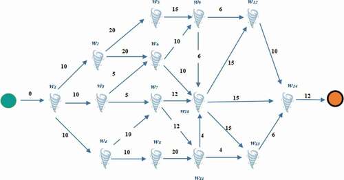
Table 2. Hurricane various whirlwinds to consider and their duration

$W_k$	$w_1$	$w_2$	$w_3$	$w_4$	$w_5$	$w_6$	$w_7$	$w_8$	$w_9$	${w_1}_0$	${w_1}_1$	${w_1}_2$	${w_1}_3$	${w_1}_4$
$D_t$ (min)	10	20	5	10	15	10	12	20	6	15	4	10	6	12

The duration times presented in Table 2 are reproduced in the Graph G (Figure 6) in order to illustrate the specific duration time for each whirlwind and their movements.

Figure 6. Graph G showing the movement of various whirlwinds and their duration.

The set of Earliest Start Time and Latest End Time respectively for every whirlwind from the beginning of hurricane until the ending (according to the MPM method), is presented in Figure 7 and Table 3.

Table 3. Whirlwinds earliest and latest times

$W_k$	$w_1$	$w_2$	$w_3$	$w_4$	$w_5$	$w_6$	$w_7$	$w_8$	$w_9$	${w_1}_0$	${w_1}_1$	${w_1}_2$	${w_1}_3$	${w_1}_4$
Earliest Start Time $EST$	0	10	10	10	30	30	20	20	45	51	04	66	66	76
Latest End Time $LET$	30	35	35	35	45	51	51	47	66	76	70	76	76	88
$D_t$ (min)	10	20	5	10	15	10	12	20	6	15	4	10	6	12

Figure 7. Whirlwinds earliest and latest times.

The ObjectActualPaths database and their times intervals are given in Table 4.

Table 4. Database of hurricane actual paths

OAP ID	1	2	3	4	5
OAP	($w_3,w_7,{w_1}_1,{w_1}_0$)	($w_1,w_3,w_6,w_9,{w_1}_0$)	($w_4,w_8,{w_1}_1,{w_1}_0,{w_1}_3$)	($w_2,w_5,w_9,{w_1}_0,{w_1}_2$)	($w_6,{w_1}_0,{w_1}_2$)
[$EST,LET$]	[10,76]	[0,76]	[10,76]	[10,76]	[30,76]

The process starts by representing the set of length-1 whirlwinds patterns (W₁) and the set of length-1 large patterns (L1). Then, as a second step of the process, $W_2$ is found using the object generation algorithm and $L_1$ is used in this process. Next, the supports of these whirlwinds are counted and the patterns, which have a support value larger than $suppmin$ will be assigned to the set $L_2$. Once having the sets $L_2$, $W_3$ resulting from the object generation algorithm, then the large patterns in $W_3$ are assigned to the set $L_3$. When obtaining $L_3$,$W_4$, resulting from the object generation algorithm, then the large patterns in $W_4$ are assigned to the set $L_4$. Unfortunately, none of these patterns have a support larger than $sup{p}_{min}$. This fact indicates that $L_6$ does not contain any patterns. Therefore, the Object Mobility Pattern mining algorithm terminates with the set of large whirlwinds (L).

Generation of Spatiotemporal Mobility Rules

The second phase of our proposed moving object future position prediction approach is the generation of the spatiotemporal mobility rules. In the previous phase, we defined object mobility patterns that were mined from the history of hurricane trajectories. The aim of this step is to extract mobility rules from those patterns. We suppose that we have an Object Mobility Pattern W = ($w_1$,$w_2$, …,$w_k$) during time interval [$ES{T_w}_1,LE{T_w}_k$], where k ¿ 1, then we extract all the mobility rule possibilities, which can be obtained from the above-mentioned pattern. We call the part of the rule before the arrow the head of the rule, and the part after the arrow the tail of the rule. An example is proposed as follows:

($w_1$,[$ES{T_w}_1,LE{T_w}_1$]) $\to$ ($w_2$, …,$w_k$ [$ES{T_w}_2,LE{T_w}_k$])

($w_1$,$w_2$,[$ES{T_w}_1,LE{T_w}_2$]) $\to$ ($w_3$, …,$w_k$,[$ES{T_w}_3,LE{T_w}_k$])

… …

($w_1$,$w_2$,$w_3$,$w_{k-1}$,[$ES{T_w}_1,LE{T}_{wk-1}$]) $\to$ ($w_k$,[$ES{T_w}_k,LE{T_w}_k$])

Furthermore, after the generation of these rules, we have to count the value that we can use to construct a confidence interval. This latter is used to found the error margin for all possible mobility rules by using the mined Object Mobility Patterns. A comparative analysis will be applied in the next step in order to extract the rules that have a higher confidence than the predefined confidence threshold.

For a mobility rule MR

($w_1$, $w_2$, $w_3$, …, $w_{r-1},[ES{T_w}_1,LE{T}_{wr-1}]$) $\to$ ($w_r$, $w_{r+1}$, …, $w_k,[ES{T_w}_r,LE{T_w}_k]$), the confidence is obtained according to the following formula:

(5) $Confidence(MR)=\frac{(w_1,w_2,w_3,\dots ,w_K,[ES{T_w}_1,LE{T_w}_k]).count}{(w_1,w_2,w_3,\dots ,w_r{{ }_{-}}_1,[ES{T_w}_1,LE{T}_w{{{ }_k}_{-}}_1]).count}\times 100$(5)

The mined Object Mobility Patterns allow us determining all the confidence values and then generate the possible mobility rules. Then, we select the rules having higher confidence (compared to the predefined confidence threshold $(con{f}_{min})$), to be used next in the mobility prediction algorithm.

The Prediction of Moving Object’s Future Position

After selecting the rules, we will pass to the third and the last phase, where the future position of the hurricane will be predicted. The prediction methodology can be outlined as pursues:

Expect that a hurricane has pursued a trajectory T =($w_1$, $w_2$, $w_3$, …, $w_{r-1}$) up to now. Our proposed methodology discovers the rules whose head parts are contained in trajectory T and furthermore the last whirlwind in their head $w$. We consider these rules the matching ones, which define how duplicate records are identified in duplicate rules. We store the primary whirlwind of the tail of each matching rule alongside a value, which is determined by summarizing the confidence and the support values of the rule in an array of such tuples. The support of a rule is the support of the Object Mobility Pattern from which the present rule is produced. The tuples of this array are then arranged in sliding request as for their support in addition to confidence values. While arranging the matching rules, both the support and confidence values of a rule ought to be thought about to choose the most confident and continuous rules. At that point, we characterize another parameter m, which is the greatest number of forecasts that can be made each time the hurricane moves. For prediction, we pick out the primary m tuples from the arranged tuples array. At that point, the whirlwinds of these tuples are our predictions for the following path of the hurricane. It implies that we utilize the primary m matching rules that have the most elevated confidence in addition to support esteem for predicting hurricane next location.

Algorithm 5 details the steps of our movement prediction model.

Algorithm 5 Moving object future position prediction algorithm

Input: Topical trajectory of the moving object,$T=(w_1,w_2,w_3,..,w_{i-1})$

Set of movement rules,$MR$

The greatest number of predictions that can be made each time,$m$

Output: The predicted future position, $FP$

1: $PN$= $\mathrm{\varnothing }$ ▹ Initially, the set of predicted moving objects is void

2: $K=1$

3: for each rule $r:(y_1,y_2,y_3,\dots .,y_u,[ES{T_y}_1,LE{T_y}_u])$ $\to (y_{u+1},y_{u+2},\dots .,y_i,[ES{T}_{yu+1},LE{T}_{yi}])\in MR$ do ▹ check all the rules in $MR$ find the set of matching rules

4:   if $(y_1,y_2,y_3,\dots .,y_u,[ES{T_y}_1,LE{T_y}_u])$ $iscontainedby$ $\mathrm{T}=(w_1,w_2,w_3,..,w_{i-1},[ES{T}_{w1},LE{T_w}_{i-1}])$ and $y_u=w_{i-1}$ then

5:     $MatchingRules\leftarrow MatchingRules\cup r$ ▹ Add the rules into the set of matching rules

6:     $TupleArray[k]=(y_{u+1},r.confidence+r.support)$ ▹ Add the $(y_{u+1},r.confidence+r.support)$ tuple to the Tuples array

7:     $K=k+1$

8:   end if

9: end for

10: $TupleArray\leftarrow \sqrt{TupleArray}$ ▹ Sort the tuples array to the second element of the tuples that is the confidence in descending order

11: $index=0$

12: while ($index<m$ && $index<TupleArray.length$) do ▹ select the first m elements of the TuplesArray

13:   $PC\leftarrow PC\cup TuplesArray[index]$

14:   $index=index+1$

15: end while

16: return $FP$

Now, let us suppose that the hurricane is moving during the whirwinds shown in Figure 5, as well the ObjectActualPaths that the hurricane has followed during its movement history are given in Table 4. To reach the desired result, we will use the mobility rules.

Furthermore, assume that the hurricane whirlwinds passed through a path $P=w_2,w_3,w_0,w_{10}$ up to now and he is actually in whirlwind $w_{10}$. Our proposed algorithm will discover the rules $(w_{10})\to (w_{12})$,$(w_{10})\to (w_{13})$, $(w_6,w_{10})\to (w_{12})$, $(w_9,w_{10}\to (w_{12}$), and ($w_5,w_9,w_{10})\to (w_{12})$ as the matching rules. The first whirlwind in each rule tail will be stocked over with the rules confidence plus support value in an array of (whirlwind, confidence + support) tuples. For our example, the resulted tuple array will be as follows:

[($w_{12}$,52), ($w_{13}$,26), ($w_{12}$,67.6), ($w_{12}$,51), ($w_{12}$,101)]

If there are more than one tuple for a whirlwind in the array, then the one which has the biggest value of the sum (confidence + support) will be kept and the others will be deleted. The kept tuples are sorted in descending order according to the value resulting from the sum of confidence and the support values.

For our example, the sorted tuple array will be: TupleArray = [($w_{12}$,101), ($w_{13}$,26)]. If m is equivalent to 1, at that time only whirlwind $w_{12}$ will be used in the prediction of hurricane future movement. If m is equivalent to 2, then both whirwinds $w_{12}$ and $w_{13}$ are the predicted whirlwinds for the future movement.

Results and Evaluation

Dataset Description

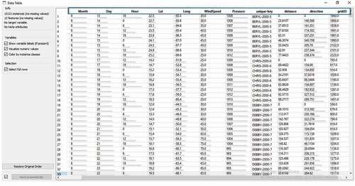
Test is an important phase that enables us to evaluate and to measure the efficiency of our approach. It evaluates and proves the efficiency of our system. For this reason, we used a real-world hurricane dataset. In fact, we used a comprehensive weather data and analytic services and solutions Unisys Weather Atlantic raw Hurricane dataset,¹ which has more than 30 years of providing reliable and timely weather data and products to the global weather enterprise, public, weather-sensitive industries and businesses, and governments.

The data was extracted from the National Hurricane Center (NHC) of the National Oceanic and Atmospheric Administration (NOAA)² that maps the oceans and conserves their living resources; predicts changes to the earth’s environment; provides weather reports and forecasts floods and hurricanes and other natural disasters related to weather. The data contains 13131 instances. The volume of the used dataset is huge, for this reason, we decided to split the dataset and selected only 3775 instances for the test phase. The dataset contains 12 features related to hurricanes like latitude and longitude in tenths of degrees, as well as the wind speeds (in knots where one knot is equal to 1.15 mph) and minimal central pressure (in millibars) for the life of the historical track of each cyclone. Our work estimates only hurricanes’ futureposition based on spatiotemporal variables plus environmental or climate variables such as sea-surface temperature, vertical wind shear, maximum winds, the radius of maximum wind and central pressure. The mentioned features and the rest of them are shown in Figure 8.

Figure 8. Hurricane features.

As a first step, we need to visualize the dataset instances as a graph. To do so, we choose to use Gephi³ as data Visualization Software. This is used by scientists and data analysts and allow them to interact with all kinds of graphs, manipulate the shape, structures, and colors easily.

Furthermore, it helps users intuitively in discovering patterns, making hypothesis, isolating structure singularities.

We imported our hurricane Dataset in Gephi. Nodes (whirlwinds) position were random at the begining, that is why we can see a slightly different representation. In order to make esthetically pleasing representation, we need to adjust the algorithm from the layout properties.

Outlier Detection

In order to generate whirlwinds actual paths, a number of whirlwinds mobility patterns were generated.

We note that there are two types of generated whirlwinds actual paths. The first type concerns whirlwinds actual paths that follow a whirlwinds mobility pattern. They are called inliers and the second type concerns the whirlwinds actual paths that do not follow a whirlwinds mobility pattern. They are called outliers.

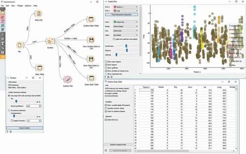
In order to have the both types separately, we use Orange,⁴ which is a data visualization and analysis tool, where data mining is done through visual programming or Python scripting.

The outliers were detected by comparing distances between instances. We choose the one-class SVM with non-linear kernel (RBF) method, with Nu set at 20 (less training errors, more support vectors).

Then, we observed the outliers in the data table widget, while we sent the inliers to the scatter plot (Figure 9).

Figure 9. Outlier detection.

The ratio of the number of outliers to the number of whirlwind actual paths that follow a whirlwinds mobility pattern is denoted by 0. For each new whirlwind actual path, we decide if it will be considered as an outlier or not, according to the value 0. If it is an outlier, then it is formed as a random walk over the hexagonal network. Otherwise, a whirlwind mobility pattern will be selected randomly and will be considered as the generated whirlwind actual path.

The total number of generated whirlwinds actual paths is 3775. From those latter, we construct the training set and the test set. The number of whirlwinds actual paths in training set is 1925 and the number of whirlwinds actual paths in test set is 1850. Whirlwinds mobility patterns are mined from the whirlwinds actual paths in the training set and then the mobility rules that will be used in prediction are generated by using these whirlwinds mobility patterns. The whirlwinds actual paths in the test set are used for evaluating the prediction accuracy of our algorithm.

There are three possible outcomes for the future location prediction, when compared to the actual location position:

• The predictor correctly identified the location of the next move.

• The predictor incorrectly identified the location of the next move.

• The predictor returned “no prediction”.

The parameters used in the experiments and their default parameters values are given in Table 5.

Table 5. Prediction of experimental parameters

Symbol	Definition	Default values
m	Maximum number of predictions	2
o	Outlier percentage	50.99%
$Sup{p}_{min}$	Minimum support percentage	0.09%
$Con{f}_{min}$	Minimum confidence percentage	70%

First, we chose m (the maximum number of predictions made each time) value, which is appropriate for all approaches. Next, we fixed the parameters of our approach: $sup{p}_{min}$ (the minimum support threshold used in Object Mobility Pattern Mining algorithm) and $con{f}_{min}$ (the minimum confidence threshold used in mobility rule generation algorithm). Finally, we extracted the outliers percentage to measure the performance of our approach as compared to the performance of other approaches.

ObjectMobilityPattern Approach Performance Metrics and Evaluation

The evaluation was made according to standard effectiveness measures that are the precision, the recall and the F-measure.

The precision measures the system’s efficacy by measuring the number of correctly predicted whirlwinds results divided by the total number of the made predictions. It is given by the following formula:

(6) $Precision=\frac{CorrectlyPredictedWhirlwinds}{TotalPredictions}$(6)

The recall measures the system’s efficacy by measuring the percentage of correctly predicted whirlwinds results divided by the total number of requests (i.e., the total number of hurricane inter-whirlwind movement). Thus, the recall counts the “no-prediction” case as an incorrect prediction. It is given by the following formula:

(7) $Recall=\frac{CorrectlyPredictedwhirlwinds}{TotalRequests}$(7)

The Bias: Precision and recall must usually be balanced with each other. In fact, increasing precision leads to decrease the recall, and vice versa. Therefore, the best measure of the overall performance of the classifier considers both precision and recall. However, if our approach results are heavily biased toward precision or recall, these combined scores may be misleading because this can produce quite high scores while still producing results that may not be acceptable to the end user. The bias score highlights this shortcoming and is given by the following formula:

(8) $Bias=\frac{CorrectlyPredictedWhirlwinds+TotalPredictions}{CorrectlyPredictedWhirlwinds+TotalRequests}$(8)

The CSI is a measure of overall classification performance. It is the Critical Success Index, also known as the threat score. This latter is similar to precision and recall, but it will be penalized for a large number of false alarms and missed the positive number in the denominator. The CSI is given by the following formula:

(9) $CSI=\frac{CorrectlyPredictedWhirlwinds}{CorrectlyPredictedWhirlwinds+TotalPredictions+TotalRequests}$(9)

The F-measure is used to create a compromise between the precision and the recall since they vary inversely, by combining them. It is given by the following formula:

(10) $F-measure=\frac{2\ast (Precision\ast Recall)}{(Precision+Recall)}$(10)

Table 6 regroups our approach test results for the dataset versus the associative classification approach. Our goal is to predict the future location of hurricane. We compared our Object Mobility Pattern Mining spatiotemporal mobility prediction approach to the mobility prediction based on Associative Classification method (Jankulak 2012).

Table 6. Results

Parameters	ObjectMobilityPattern					Associative Classification
	Precision	Recall	Bias	F-measure	CSI	Precision	Recall	F-measure
$m=1$	0.39	0.17	0.47	0.23	0.13	0.37	0.42	0.40
$m=2$	0.23	0.175	0.73	0.19	0.11	0.20	0.21	0.20
$m=3$	0.20	0.18	0.74	0.19	0.10	0.15	0.16	0.15

This latter has aims to customize the prior-based association rules algorithm to produce rules that could be combined into an associative classifier for predicting hurricane next position. An associative classifier is composed of two parts: a class-targeted form of Association Rule Mining (ARM) to produce Class Association Rules (CARs), and a strategy to build a classifier by selecting and ordering these rules and specifying a default class for those cases that are not matched by any rule.

When we examine the performance impact of parameter m, maximum number of predictions made at each move of whirwind, we conclude that the precision value obtained by our approach and the precision obtained by Associative Classification approach decrease as m increases. The decrease in both precision values is due to the fact that as the number of predictions made at each movement of whirwinds increases, the probability of having some incorrect predictions increases too. The precision obtained by our approach shows a better result when compared to this obtained by associative classification method. The recall values for both methods increase when m increases. This fact can be explained by the fact that as the number of predictions made at each move of hurricane increases, the probability of predicting the correct whirwind increases. The increase in recall values with Associative Classification approach is more significant when compared to the increase with our approach. In fact, for our approach the recall values do not increase significantly due to the fact that the number of matching rules is the same for all m values.

After making use of the three most used effectiveness measures, we decided to evaluate our approach on the basis of running time.

In Figure 10, we have two curves that take the size of the dataset (expressed in the number of tested instances) as abscissa and the corresponding run time (espressed in milliseconds) as coordinates. The blue one expresses the variation of the run time compared to the size of the used dataset using our approach. The orange one expresses the variation of the run time compared to the size of the used dataset using the associative classification approach. This representation facilitates the comparison between the two approaches in terms of running time.

Figure 10. Run time ObjectMobilityPattern approach versus AssociativeClassification approach.

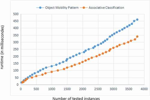
We started by testing only 500 instances and we recorded the corresponding run time. Then, we incremented the instances by adding 500 instances each time until completing the whole 3775 total instances.

We note that the curves show that our approach takes more running time compared to the associative classification approach. This is due to the fact that our proposed approach takes into consideration the temporal, the spatial and the semantic aspects, whereas the associative classification approach takes into consideration only the spatial aspect. Thus, increases automatically the treatment time.

Conclusion

Nowadays, the prediction models become the main way to predict moving object’s future positions. The need of predictive models for tracking moving objects trajectories becomes more and more crucial. In fact, being able to predict a moving object’s future position related to natural phenomena, would allow decision makers to take strategic decisions in order to help the humanity, and prevent or avoid the propagation of natural catastrophes. Scientists have greatly improved the nation’s capability to predict most natural catastrophes and disseminate warnings based on those predictions. By this way, people can act to protect themselves from injury, economic losses and death. When the future position of a moving disaster such as hurricane is predict in advance, lives, properties and natural resources can be protected. Therefore, predicting the future position of hurricanes is a real challenge. This was our motivation in this paper. In fact, we proposed to predict the pattern of movement of hurricanes from its previous trajectory data for that, we presented a new data mining approach, for predicting hurricanes’ future positions. The proposed approach is composed of three phases. The first step is to consider each object (hurricane) move over a time period extracted from the history of hurricane trajectories. Thereafter, object mobility patterns are mined. In the second phase, spatiotemporal mobility rules are extracted from these patterns. In the last phase, moving object (hurricanes) future positions predictions are accomplished by using these rules. In the experimentation, we used NOAA dataset that is composed of 3775 instances. Then, we evaluated our approach by using the most used effectiveness measures such as the Precision, the Recall and the F-measure. Our approach showed promising results comparing to the Associative Classification approach. As future work, we propose to support real-time analysis and prediction alerts in case of major risks and to make the approach more efficient by predicting the whole trajectory instead of predicting only the future position. By tracking the future position of hurricanes, we intend to add other parameter values to find out the severity and the intensity of hurricanes such as the eye diameter (nm), the pressure of the outermost isobar (hpo), the radius of the outermost closed isobar (nm), the radius of maximum wind velocity (nm) and the distance to the nearest land (nm).

Disclosure statement

No potential conflict of interest was reported by the author(s).

Notes

1. http://weather.unisys.com/hurricane/atlantic/.

2. https://www.nhc.noaa.gov.

3. https://gephi.org/.

4. https://orange.biolab.si/.

References

- Alemany, S., J. Beltran, A. Perez, and S. Ganzfried, 2018a. Predicting hurricane trajectories using a recurrent neural network. arXiv preprint arXiv:1802.02548.
- Alemany, S., J. Beltran, A. Perez, and S. Ganzfried. 2018b. Predicting hurricane trajectories using a recurrent neural network. Proceedings of the AAAI Conference on Artificial Intelligence 33.
- Ayat, H., J. Evans, and A. Behrangi. 2021. How do different sensors impact imerg precipitation estimates during hurricane days? Remote Sensing of Environment 259:112417. doi:https://doi.org/10.1016/j.rse.2021.112417.
- Camargo, S., A. Robertson, S. Gaffney, P. Smyth, and M. Ghil. 2007. Cluster analysis of typhoon tracks. part i: General properties. Journal of CLIMATE - J CLIMATE 20(14) .
- Castelli, M., L. Vanneschi, and A. Popovič. 2015. Predicting burned areas of forest fires: An artificial intelligence approach. Fire Ecology 11 (1):106–18. doi:https://doi.org/10.4996/fireecology.1101106.
- Chen, M., X. Yu, and Y. Liu. 2016. Mining object similarity for predicting next locations. Journal of Computer Science and Technology 31 (4):649–60. doi:https://doi.org/10.1007/s11390-016-1654-2.
- Cook, D. L., 1966. Program evaluation and review technique–applications in education.
- Council, N. R., et al. 1991. A safer future: Reducing the impacts of natural disasters. Washington, DC: National Academies Press.
- DeMaria, M., and J. Gross, 2013. Evolution of prediction models. pp. 103–26.
- Goerss, J., C. Sampson, and J. Gross. 2004. A history of western north pacific tropical cyclone track forecast skill. Weather and Forecasting 19 (3):633–38. doi:https://doi.org/10.1175/1520-0434(2004)019<0633:AHOWNP>2.0.CO;2.
- Gusfield, D. 1997. Algorithms on strings, trees, and sequences. In Computer science and computational biology. 1-326. New York: Cambridge University Press.
- Güting, R. H., and M. Schneider. 2005. Moving objects databases. Morgan Kaufmann Publishers In.
- Hall, T. M., and S. Jewson. 2007. Statistical modelling of north Atlantic tropical cyclone tracks. Tellus A: Dynamic Meteorology and Oceanography 59 (4):486–98. doi:https://doi.org/10.1111/j.1600-0870.2007.00240.x.
- Hoang, M. X., Y. Zheng, and A. K. Singh, 2016. Fccf: Forecasting citywide crowd flows based on big data, in: Proceedings of the 24th ACM SIGSPATIAL International Conference on Advances in Geographic Information Systems, ACM, california. p. 6.
- Ishikawa, Y., Y. Tsukamoto, and H. Kitagawa, 2004. Extracting mobility statistics from indexed spatio temporal datasets, in: STDBM, Toronto, pp. 9–16.
- Jankulak, M. L., 2012. Prediction of rapid intensity changes in tropical cyclones using associative classification.
- Kowaleski, A., and J. Evans. 2020. Use of multiensemble track clustering to inform medium-range tropical cyclone forecasts. Weather and Forecasting 35: 4.
- Landsea, C., and J. Cangialosi. 2018. Have we reached the limits of predictability for tropical cyclone track forecasting? Bulletin of the American Meteorological Society 99: 11.
- Marks, F., L. Shay, G. Barnes, P. Black, M. Demaria, B. McCaul, J. Mounari, M. Montgomery, M. Powell, J. Smith, et al. 1998. Landfalling tropical cyclones: Forecast problems and associated research opportunities. Bulletin of the American Meteorological Society 79:305–23.
- McDermott, P. L., and C. K. Wikle. 2019. Bayesian recurrent neural network models for forecasting and quantifying uncertainty in spatial-temporal data. Entropy 21 (2):184. doi:https://doi.org/10.3390/e21020184.
- Monreale, A., F. Pinelli, R. Trasarti, and F. Giannotti, 2009. Wherenext: A location predictor on trajectory pattern mining, in: Proceedings of the 15th ACM SIGKDD international conference on Knowledge discovery and data mining, ACM, Paris, France. pp. 637–46.
- Nanopoulos, A., D. Katsaros, and Y. Manolopoulos, 2001. Effective prediction of web-user accesses: A data mining approach, in: Proceedings of the WEBKDD Workshop, Poland.
- Nanopoulos, A., D. Katsaros, and Y. Manolopoulos. 2003. A data mining algorithm for generalized web prefetching. IEEE Transactions on Knowledge & Data Engineering 15 (5):1155–69. doi:https://doi.org/10.1109/TKDE.2003.1232270.
- Oueslati, W., and J. Akaichi. 2010. Mobile information collectors trajectory data warehouse design. International Journal of Managing Information Technology (IJMIT) 2 (3):1–20. doi:https://doi.org/10.5121/ijmit.2010.2301.
- Qiao, S., D. Shen, X. Wang, N. Han, and W. Zhu. 2015. A self-adaptive parameter selection trajectory prediction approach via hidden Markov models. IEEE Transactions on Intelligent Transportation Systems 16 (1):284–96. doi:https://doi.org/10.1109/TITS.2014.2331758.
- Raschky, P. A. 2008. Institutions and the losses from natural disasters. Natural Hazards and Earth System Sciences 8 (4):627–34. doi:https://doi.org/10.5194/nhess-8-627-2008.
- Roy, B. 1971. Problems and methods with multiple objective functions. Mathematical Programming 1 (1):239–66. doi:https://doi.org/10.1007/BF01584088.
- Wiest, J., M. Höffken, U. Kreßel, and K. Dietmayer, 2012. Probabilistic trajectory prediction with Gaussian mixture models, in: 2012 IEEE Intelligent Vehicles Symposium, IEEE, Madrid, Spain. pp. 141–46.
- Willoughby, H., E. Rappaport, and F. Marks. 2005. Hurricane forecasting: The state of the art. Natural Hazards Review 8.
- Yang, J., and M. Hu, 2006. Trajpattern: Mining sequential patterns from imprecise trajectories of mobile objects, in: International Conference on Extending Database Technology, Springer, Munich, Germany. pp. 664–81.
- Yavaş, G., D. Katsaros, Ö. Ulusoy, and Y. Manolopoulos. 2005. A data mining approach for location prediction in mobile environments. Data & Knowledge Engineering 54 (2):121–46. doi:https://doi.org/10.1016/j.datak.2004.09.004.
- Ying, J. J. C., W. C. Lee, and V. S. Tseng. 2013. Mining geographic-temporal-semantic patterns in trajectories for location prediction. ACM Transactions on Intelligent Systems and Technology (TIST) 5:2.
- Zhao, Y., R. Yang, G. Chevalier, R. C. Shah, and R. Romijnders. 2018. Applying deep bidirectional LSTM and mixture density network for basketball trajectory prediction. Optik 158:266–72. doi:https://doi.org/10.1016/j.ijleo.2017.12.038.
- Ziliani, L., and N. Surian. 2016. Reconstructing temporal changes and prediction of channel evolution in a large alpine river: The tagliamento river, Italy. Aquatic Sciences 78 (1):83–94. doi:https://doi.org/10.1007/s00027-015-0431-6.