Prediction of Local Scour around Bridge Piers Using Hierarchical Clustering and Adaptive Genetic Programming

ABSTRACT

The physics of local scour around bridge piers is fairly complex because of multiple forces acting on it. Existing empirical formulas cannot cover all scenarios and soft computing methods require ever greater amounts of data to cover all cases with a single formula or a neural network. The approach proposed in this study brings together observations from over 40 studies, grouping similar observations with hierarchical clustering, and using genetic programming with adaptive operators to evolve formulas specific to each cluster to predict the scour depth. The resulting formulas are made available along with a basic web-based user interface that finds the closest cluster for newly presented data and finds the scour depth using the formula for that cluster. All formulas have R² scores over 0.8 and have been validated with validation and testing sets to reduce overfitting. When compared to existing empirical formulas, the generated formulas consistently record higher R² scores.

Introduction

According to statistical studies, the most common cause of bridge failure is the floods that scour the bed material around the bridge piers (Hoffmans and Verheij 1997; Richardson and Davis 2001). Many researchers are interested in the prediction of scour depth around piers to maximize the benefits of hydraulic structures and to reduce the damage caused. Scour prediction is challenging because of the multiple uncertainties involved in the process, such as time-dependent three-dimensional flow patterns, vorticities, and the phenomena of sediment transport.

Prediction requires experience in several fields of engineering, an understanding of the behavior of water flow, and the interaction between the water, the structures and the soil. Extensive laboratory experiments have been conducted to observe and to predict the equilibrium local scour depth (Chabert and Engeldinger 1956; Melville 1975, 1997; Ettema 1980; Yanmaz and Altinbilek 1991; Melville and Chiew 1999; Oliveto and Hager 2002; Coleman, Lauchlan, and Melville 2003; Yanmaz 2006; Hager and Unger 2010; Lan¸ca et al. 2013; Bor 2015; Sheppard, Melville, and Demir 2014; Vijayasree et al. 2019).

These experiments yielded equations based on the correlation of small-scale data obtained from laboratory experiments, which aim to reduce the complexity of on-site conditions. Experimental laboratory data are used in these equations, therefore they can only predict prototype scour depths under similar conditions, and they are not universal. It is difficult to represent a real river and bridge pier system in a laboratory flume, so several assumptions are incorporated in laboratory studies. Recording real-time observations are the ideal for understanding the complexity of real-life river systems, however, these are very challenging or sometimes impossible to conduct in the field.

With the availability of more data and more accessible machine learning algorithms, the focus has shifted to alternative approaches such as regression methods, artificial neural networks (ANNs) (Azamathulla et al. 2010; Azmathullah, Deo, and Deolalikar 2005; Bateni, Borghei, and Jeng 2007; Firat and Gungor 2009; Jain 2001; Kaya 2010; Lee et al. 2007; Liriano and Day 2001; Mohammadpour, Ghani, and Azamathulla 2013) and evolutionary computation (EC) (Azamathulla et al. 2010; Guven, Azamathulla, and Zakaria 2009). These methods can be used to estimate scour depth with a number of reliable data sets, making them useful in modeling problems in which there is a deficient understanding of the relationship between the dependent and independent variables.

This study uses a combination of equilibrium scour depth observations from laboratory experiments, and field measurements from the literature. Since these observations are obtained from various setups, they are grouped by hierarchical clustering so that similar observations from different studies could be used together. A formula has been evolved for each cluster using values from the data sets, constants, variables, and modified mathematical functions. When a new prediction is needed, first the closest cluster should be found, and then the formula for that cluster should be used. These two steps are handled with a basic client-side JavaScript application that has been made available online.

The rest of the manuscript is structured as follows: The next section discusses existing studies on the problem. Section 3 details the parameter selection for scour depth prediction and the data. The method is discussed in Section 4 and the results are given and evaluated in Section 5. Section 6 includes concluding remarks.

Related Work

In practice, the pier scour depth is predicted by formulas produced from evaluations of the data collected from empirical observations. The three most used are by Jain and Fischer (Jain and Fischer 1979), by Melville (Melville 1997), and by Richardson and Davis, known as HEC-18 (Richardson and Davis 2001). Since these formulations are conservative and produce safe results for a range of values outside of their initial scope, researchers have instead turned to soft computing methods.

Soft computing methods require data for their training. Data is available in the literature, but three main points have to be considered before they are considered suitable for a study. Foremost, data collected at fixed time intervals are out of scope for studies that use the equilibrium scour depth, as in this study. Second, approaches taken to scour depth prediction depend on their usage of dimensional and dimensionless variables. Finally, not all studies use the same evaluation criteria to report their findings. These issues make it very challenging to make comparisons. Nevertheless, all these studies provide valuable information because they report the effectiveness of their approaches, the variables that are more significant, and the performance of the hyper parameters of used soft methods.

To the best of our knowledge, genetic programming was first applied to scour depth prediction in the works of Guven et al. who found out that linear genetic programming (LGP) performs much better than adaptive neuro-fuzzy inference system (ANFIS) (Guven, Azamathulla, and Zakaria 2009). Their study was continued with a follow-up paper which compared GP with radial basis function neural network using 398 observational data (Azamathulla et al. 2010). They reported an R² score of 0.819 for GP where ANN scored 0.691. Wang et al. found that GP performs better than existing empirical formulas on a data set of 130 observations (Wang et al. 2013). Najafzadeh and Barani incorporated GP and ANN to come up with two models of group method of data handling (GMDH) (Najafzadeh and Barani 2011). They reported that GMDH-GP provided better results than the ANN-based GMDH, but also had the disadvantage of being more time consuming and more complicated.

Besides GP, there are approaches that use artificial neural networks (ANN) (Cheong 2006; Firat and Gungor 2009; Kaya 2010; Trent, Gagarin, and Rhodes 1993), ANN with adaptive ANFIS (Choi, Choi, and Lee 2017), particle swarm optimization to optimize ANN parameters (Dang, Anh, and Dang 2019), deep neural networks (Pal 2019) and an extension of support vector machines (Pal, Singh, and Tiwari 2011). Two recent surveys provide more detailed information on the field. The survey by Sharafati et al. provides an overall comparison of all soft computing methods with empirical formulas (Sharafati et al. 2019), while the one by Pizarro et al. covers not just the methods but also the physical phenomena that affects the scours in bridge foundations (Pizarro, Manfreda, and Tubaldi 2020).

It is important to emphasize that although GP performs as well as, or even better than other soft computing methods, it is less commonly used as ANN. We believe this is because the adjustment of its hyper parameters requires a high level of fine tuning in mathematical functions, and the time needed to reach a successful outcome. Another reason is that the lack of programming libraries make it more difficult to use. This difficulty has been overcome by the DEAP framework, which simplifies the underlying algorithms for manipulating tree-based structures during crossover and mutation (Fortin et al. 2012). However, the configuration required is substantially greater than for existing point and click graphical user interfaces available for ANNs.

Data

Data Sets

There are two sources of data; we refer to the observations obtained from real-life river systems as field data, and those obtained from flume experiments in a laboratory setup as laboratory data. Field data is better at explaining the real-life systems than laboratory data, but it is very challenging to collect. Laboratory conditions make data collection easier, but they cannot completely reflect the complexity of real-life river systems.

There are two types of scouring depending on the transport mode of the sediment. Clear-water scour occurs when sediment is removed from the scour hole, but not transported to other parts of the bed through the flow. Live-bed scour occurs when flow transports the sediment particles to other parts of the bed. Both conditions can be replicated in laboratory experiments. Therefore, the data sets are categorized into four: field clear-water, field live-bed, laboratory clear-water, and laboratory live-bed.

The data selection from the existing literature has been evaluated with the following criteria.

• Short-term data were discarded.

• All data were selected from the experiments for the middle circular piers.

• All experiments were selected under equilibrium conditions.

• All pier angles were chosen parallel to the flow direction.

• The data is divided into two categories; field and laboratory. Each category is also divided into two sub-categories clear-water scour and live-bed scour.

This study brings together 23 field data sets found in the literature, as listed in Table 1. These combined data yields a total of 775 field live-bed and 592 field clear-water observations.

Table 1. Field scour data sources in literature that are used in this study

Field Data	Live-bed	Clear-water
Bata and Todorovic (1960)	2	–
Benedict and Caldwell (2006)	4	–
Benedict and Caldwell (2009)	16	–
Boehmler and Olimpio (2000)	–	9
Breusers, Nicollet, and Shen (1977)	1	–
Butch (1991)	16	35
Chang (1980)	6	–
C. Watt, (USGeologicalSurvey 2001 (in 2014 press))	7	8
Davoren (1985)	10	–
Gao, Posada, and Nordin (1993)	249	237
Hayes (1996)	37	80
Hodgkins and Lombard (2002)	1	11
Holnbeck (2011)	1	8
Hopkins, Vance, and Kasraie (1980)	1	–
NBSD (USGeologicalSurvey 2001)	143	98
Muller, Miller, and Wilson (1994)	17	–
Muller and Wagner (2005)	140	96
Neil (1965)	1	–
Shen (1975)	–	3
Southard (1992)	3	–
Williamson (1993)	2	6
Wilson (1995)	36	–
Zhuravlyov (1978)	82	1
Total	775	592

There are 24 laboratory data sets as listed in Table 2 with a total of 233 laboratory live-bed and 596 laboratory clear-water observations.

Table 2. Experiment scour data sources in literature that are used in this study

Experiment Data	Live-bed	Clear-water
Aksoy et al. (2017)	–	16
Chabert and Engeldinger (1956)	12	81
Chee (1982)	36	1
Chiew (1984)	92	9
Coleman (unpublished)	3	3
Dey, Bose, and Sastry (1995)	–	18
Dey and Raikar (2005)	–	16
Ettema (1980)	1	96
Ettema et al. (2006)	–	6
Ettema (1976)	–	19
Graf (1995)	–	3
Jain and Fischer (1979)	30	4
Jones (unpublished)	1	16
Lan¸ca et al. (2013)	–	38
Melville (1997)	–	17
Melville and Chiew (1999)	–	27
Mignosa (1980)	–	13
Oliveto and Hager (2002)	15	73
Pandey et al. (2018)	–	4
Pandey et al. (2019)	–	85
Shen, Schneider, and Karaki (1969)	21	2
Max and Miller (2006)	20	4
Max, Odeh, and Glasser (2004)	2	12
Yanmaz and Altinbilek (1991)	–	33
Total	233	596

One of the key parts of our study is collating a large number of data sets and processing them for analysis, providing a large range of values for use in the construction and evaluation of soft computing methods. Even with such large data, several parameters that affect the local scour around the piers, needed to be taken into account before the data could be used to estimate the scour depth.

Parameters Affecting the Local Scour around Piers

The scour depth around a pier shown in Figure 1 is influenced by various parameters, given as the relation $f_1$ in Equation 1(1) ${\mathrm{d}}_{\mathrm{s}}=f_1\left[\rho ,\upsilon ,y,u,\alpha ,g,u_{\ast },D_{50},{\sigma }_g,{\rho }_s,B,b,S_0,K_s,K_g,t\right]$(1) .

(1) ${\mathrm{d}}_{\mathrm{s}}=f_1\left[\rho ,\upsilon ,y,u,\alpha ,g,u_{\ast },D_{50},{\sigma }_g,{\rho }_s,B,b,S_0,K_s,K_g,t\right]$(1)

Figure 1. Local scour around bridge pier.

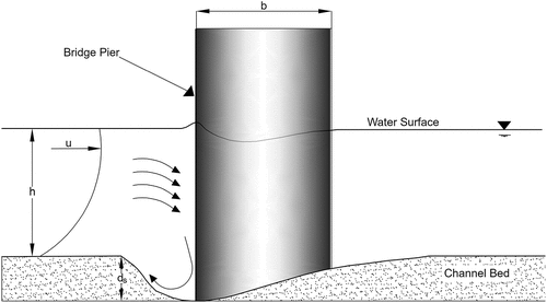
In relation $f_1$, $d_s$ is the scour depth at instant $t$; $\rho$ is the fluid density; $\upsilon$ is the kinematic viscosity; $y$ is the approach water depth; $u$ is the mean approach velocity; $\alpha$ is the angle between pier and flow direction; $g$ is the gravitational acceleration; $u_{\ast }$ is the shear velocity; $D_{50}$ is the mean sediment size; ${\sigma }_g$ is the geometric standard deviation of particle size distribution; ${\sigma }_g$ is the sediment density; $B$ is the river width; $b$ is the pier width; $S_0$ is the slope of the channel; $K_s$ is the pier shape coefficient; $K_g$ is the coefficient describing the geometry of the channel cross section; and $t$ is the time.

Dimensionless parameters are determined by considering dimensional analysis to represent the real physical problem used to determine the scour depth in laboratory-sized setups. They can be generated by Buckingham’s $\pi$ theorem using $\rho$, $u$ and $b$ as repeating variables (Zohuri 2016). The relation $f_2$ with dimensionless parameters can be written as in Equation 2(2) $\frac{d_s}{b}=f_2\left(\frac{u}{\sqrt{gy}},\frac{u{D}_{50}}{\upsilon },\frac{y}{b},\frac{u_{\ast }}{u},\frac{D_{50}}{B},\frac{ut}{b},\frac{b}{D_{50}},\alpha ,S_0,{\sigma }_g,K_s,K_g\right)$(2) (Bor 2015; Bateni, Borghei, and Jeng 2007; A. Melih Yanmaz, 2002).

(2) $\frac{d_s}{b}=f_2\left(\frac{u}{\sqrt{gy}},\frac{u{D}_{50}}{\upsilon },\frac{y}{b},\frac{u_{\ast }}{u},\frac{D_{50}}{B},\frac{ut}{b},\frac{b}{D_{50}},\alpha ,S_0,{\sigma }_g,K_s,K_g\right)$(2)

where; $F_r=u/\sqrt{gy}$, known as the Froude Number directly upstream of the pier, $R_e=u{D}_{50}/\upsilon$, known as the Reynolds Number, and $R_e=u{D}_{50}/\upsilon$ known as the average flow intensity where $I=u/u_c$ is the mean approach critical velocity. Many known effects of parameters are generally ignored for the sake of simplicity. Both the channel width and the slope is constant; there is no group effect for the flow, and the shape can be set as 1 for circular piers; the angle between flow direction and pier axis is 0. $K_g$ can be ignored for wide rectangular channels under uniform conditions (Melville 1997). It is also assumed that the final scour depth has reached to the equilibrium condition. Hence, relation $f_2$ can be expressed as the relation $f_3$ in Equation 3(3) $\frac{d_s}{b}=f_3\left(F_r,R_e,\frac{y}{b},I,\frac{b}{D_{50}},{\sigma }_g\right)$(3) .

(3) $\frac{d_s}{b}=f_3\left(F_r,R_e,\frac{y}{b},I,\frac{b}{D_{50}},{\sigma }_g\right)$(3)

This final relation, $f_3$, has six dimensionless parameters which can be used to estimate the dimensionless $d_s/b$ ratio of scour depth to pier width. Existing data sets have been processed and these ratios have been calculated for each observation.

Method

The observations in existing studies are reported by the value ranges for each parameter, to enable their approaches to be used in the design and construction of bridges within these reported ranges. However, these value ranges do not necessarily group-related conditions together; they might include more than one class of data and it is impossible to manually separate these classes. It is also apparent that it is impossible to create generalized formula suitable for all cases with the limited existing understanding of the forces acting on a bridge scour. Therefore, this study proposes an approach that first finds similar observations in multiple sets of data using clustering, and then evolves a mathematical formula for each cluster via genetic programming. An overview of the process is given in Figure 2.

Figure 2. An overview of the method, with each major step is enclosed in dotted rectangles. “Data Preparation” step is applied to all of the categories in the previous step, “Clustering” is applied to every set in the previous step, and “Genetic Programming” is applied to every cluster in the previous step.

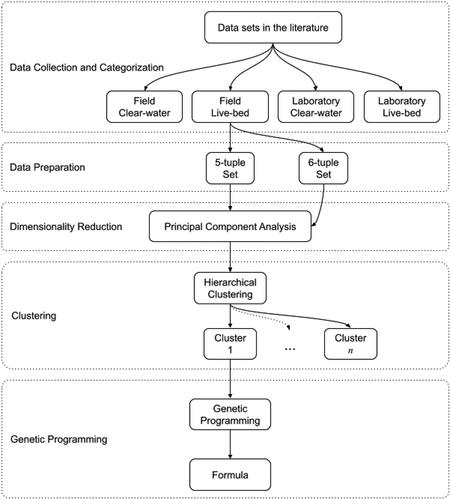
To evaluate a new observation, the nearest cluster should be first determined. Then, using that cluster’s formula, the scour depth can be predicted. Both steps in this approach requires the employment of a computer program. Because there are 32 clusters in total, a computer program makes it much easier to determine. Another advantage of the computer program is that the formulas are much easier to evaluate since genetic programming generates large and complicated formulas. Therefore, a client-side JavaScript application with a basic user interface has been developed and made available at http://homes.ieu.edu.tr/koguz/research/scour/. The cluster centers and formulas for each cluster are made publicly available in this application.

Data Categorization and Preparation

In this study, there are four major categories of observations: field clear-water, field live-bed, laboratory clear-water, and laboratory live-bed. The collected data for one category should not be used to estimate for a scour depth in another, since the physical parameters vary greatly. This step is called the “Data collection and categorization” since the categorization can be done manually with the reported properties of the data.

In Section 3.2, relation $f_3$ has been selected to determine the scour depth. This relation has six parameters which are the ratios of several parameters in the data sets. However, some of the observations in these data sets have no value for the ${\sigma }_g$ parameter. Therefore, two sets of data are created for each category; one with 5-tuple which includes the complete list of observations without the ${\sigma }_g$ parameter, and another with 6-tuple, which includes all the parameters but has fewer observations. This step is called “Data Preparation” as shown in Figure 2. At the end of these first two steps, eight sets of data are formed as listed in Table 3.

Table 3. Number of observations in each data set using 5-tuple and 6-tuple parameters

	Field		Laboratory
	5-tuple	6-tuple	5-tuple	6-tuple
Clear Water	592	399	596	580
Live-bed	775	456	233	232

The range for each parameter varies greatly, and when considered simultaneously, the larger values can dominate the result, specifically in cases where Euclidean distance is used to find the distance between points. Therefore, each dimension is normalized by the dimension’s largest value in the major category.

Principal Component Analysis

The dimensions for the 5-tuple and 6-tuple sets can be reduced by determining their principal components. Some of the dimensions in the sets may not contribute to the variance of the data. Principal component analysis (PCA) can be used to detect the dimensions that maximize the variance (Jolliffe 2005).

This is a standard statistical approach that identifies the principal components of the data by finding the eigenvectors and their corresponding eigenvalues. Each of these vectors represent one of the dimensions in the data where the eigenvalues denote how much they contribute to variance. As the data is projected to these eigenvectors, some dimensions can be omitted. Starting with the eigenvector with the largest eigenvalue, the dimensions are added until at least 90% of the data is represented. The data are then projected to the selected eigenvectors to be used during the clustering. Even though the projected values are used during clustering, the clusters are formed with the complete 5-tuple and 6-tuple original values.

Hierarchical Clustering

Clustering is the algorithmic grouping of objects in a data set in such a way that similar objects are placed in the same group in accordance with a metric, usually the Euclidean distance between them. Of the existing clustering algorithms, most require the number of expected clusters, usually denoted by k, and a number of random or existing candidate cluster centers (Xu and Tian 2015).

In cases where the number of clusters in the data is to be determined, a robust approach is to use hierarchical clustering. Hierarchical clustering requires no value for either the expected number of clusters, or any cluster centers. It begins with each object being in their own cluster, and the only element in that cluster. The algorithm joins two closest clusters at each step, until there is only one remaining cluster containing all the elements. This approach is known as agglomerative clustering (Alpaydın 2020).

Once the agglomerative clustering is complete, the original distances of two observations should be compared by the distances between the clusters they are in. This is known as the cophenetic correlation coefficient. In a valid clustering result, the ratio of the distance between two observations and the distance between their clusters should be as close to 1 as possible.

The metric used for the distances between objects affect the clustering outcome. Since the clustering process runs quickly, various metrics have been tested to obtain the most valid clustering of the data. While the Euclidean and Squared Euclidean distances were adequate for most of the sets, the field clear-water 5-tuple and 6-tuple sets yielded better results with the correlation distance and the Mahalanobis distance. The correlation distance is defined as

(4) $d=1-\frac{{\sum }_{i=1}^n\left[\left(x_s-\overline{x_s}\right)\left(x_t-\overline{x_t}\right)\right]}{\sqrt{{\sum }_{i=1}^n{(x_s-\overline{x_s})}^2{\sum }_{i=1}^n{(x_t-\overline{x_t})}^2}}$(4)

where the $\overline{x_s}$ and $\overline{x_t}$ represent the mean. The Mahalanobis distance is defined as

(5) $d=\sqrt{(y-\mu ){\sum }^{-1}{(y-\mu )}^{\mathrm{\prime }}}$(5)

which yields in the distance from vector $y$ to a distribution with mean $\mu$ and variance $\mathrm{\Sigma }$.

The resulting clusters can be visualized by a dendrogram, a tree that shows the clusters on the horizontal axis, and the connection distances on the vertical axis. The visual representation can at times provide a clear picture of the clusters, the cutoff value for the number of clusters in the data set has to be set manually by checking the number of elements in each cluster by experimenting with different values. Nevertheless, some of the observations were far away from existing groups, even at high distances. Therefore, these observations are eliminated as outliers, since they would reduce the fitness of solutions in the genetic programming step.

The eight data sets has yielded 32 clusters as listed in Table 4.

Table 4. The resulting clusters for eight data sets. F represents field data, L represents laboratory data, C represents clear-water, and B represents live-bed scour type

Data Set	C. No	C. Size		Data Set	C. No	C. Size		Data Set	C. No	C. Size
FC5	1	76		FB5	1	46		LC5	1	46
	2	38			2	49			2	127
	3	37			3	89			3	84
	4	66			4	46		LC6	1	72
	5	115			5	57			2	44
	6	47			6	38			3	287
FC6	1	35			7	104		LB5	1	69
	2	62			8	74			2	64
	3	56		FB6	1	52			3	100
	4	87			2	168		LB6	1	53
					3	37			2	89

The hierarchical clustering has been realized using MATLAB R2021b, and the resulting clusters have been exported as CSV files.

Genetic Programming

Genetic programming (GP) is an evolutionary computation method, structurally similar to genetic algorithms (GA) (Dabhi and Sanjay 2015b). Both methods borrow ideas from the theory of evolution, where fitter individuals have a better chance of breeding. The methods require a population of randomly generated solutions that are evaluated with a fitness function. The method then uses crossover and mutation operators to create the next generation of solutions. Depending on the search space of the problem, the population size and the number of generations can be adjusted to create an approximate solution. In contrast to genetic algorithms, genetic programming creates programs or formulas as solutions rather than a set of values.

This study uses a GP approach in which an individual is represented as an expression tree of mathematical functions, variables, and constants. If the node of a tree is a function, then the child nodes are its parameters. Constant values and variables are represented as leaf nodes and can be used as they are.

The aim is to find a formula that can predict scour depth using the 5-tuple or 6-tuple inputs from the data sets, as well as several mathematical functions and random constants. The random constants have been limited to floating-point values in the range of (−3,3) based on the assessment of the existing formulas in the literature. The mathematical functions addition, subtraction and multiplication have been kept as they are; however, other functions have simple modifications to control the output of the functions. Division function returns 1 if the divisor is zero. The square root function always uses the absolute value of the input, so that the function does not return a complex number. The power function sets the power value to 1 if the value is greater than 1, so that the values shrink rather than grow larger. The power function uses the absolute values for both the base and power values. Minimum function returns the minimum of two values. The tanh function returns hyperbolic tangent. A list of these primitives is given in Table 5. The absolute value of the resulting expression tree is passed to the natural logarithm function, even though it is not used within the construction of individuals.

Table 5. Our GP uses the following primitives to form its expression tree. We have modified some of the mathematical functions to control the output

Primitives for GP	Description
$F_r$, $R_e$, $\frac{y}{b}$, $I,$ $\frac{b}{D_{50}}$, ${\sigma }_g$	5-tuple or 6-tuple values acquired from the data sets
Random constants	Float values in the range ${\sigma }_g$
$+,-,\times$	Elementary arithmetical functions
$/$	Division returns 1 if the divisor is 0.
$\sqrt{\left|n\right|}$	Uses absolute value
$min\left(a,b\right)$	Returns the minimum of two values
$tanh$	Returns the hyperbolic tangent
${\left|a\right|}^{\left|b\right|}$	Uses absolute values. Returns 1 if results is greater than 1.

During the evolution of the formulas in this GP configuration, it is very likely that the expression tree will grow out of control to become very large. It is common to limit the tree depth to control this behavior. The maximum tree depth is set to 8 which has been observed to strike a fine balance between running time and memory constraints. However, the depth is increased to 16 for clusters FC5-5, FB6-2, and LB5-3 where a formula with a depth of 8 could not be obtained.

Once the individual definition is complete, GP requires a population of these individuals to start the evolution process. Due to the very large search space for the number of possible formulas that can be generated with the number of inputs and the maximum tree depth, a reasonably large number of random individuals will help the evolution process to converge to high fitness values. The initial population is therefore set to 2000. These individuals are randomly generated with the ramped half-and-half approach, which mixes the full and grow methods to increase the variety in the individuals. The trees generated by the full method has the same depth for all nodes of the tree, whereas grow method allows different sizes and shapes. Using both methods together provides the greatest likelihood of having a wide range of sizes and shapes (Poli et al. 2008).

Every generation is evaluated by a fitness function to assign fitness values to individuals. The nature of the fitness function depends on the problem itself. The fitness function in this GP configuration evaluates the mathematical expression in the individual on all of the values of the data set and calculates the coefficient of determination, better known as the R² value, to determine the fitness of each individual. R² returns a value between 0 and 1, where higher values are better. This scaled metric has provided better results than others, such as mean squared error (MSE), where the value depends on the error, because when MSE is used, there is no limit on the smallness of the error.

While the fitness value of an individual denotes how good the predictions are, it is possible that the solution might fail when new data is presented. Overfitting solutions yield very good results with the training data, but poor results with new data. The purpose of training is to generalize the solution, so that it also yields good results with previously unseen data. A common approach to reducing overfitting is to divide the available data into three disjoint sets, respectively, for training, validation, testing. This approach decreases the amount of available data for training, but reduces overfitting (Dabhi and Sanjay 2015a).

To use these sets, a metric is required to discover whether the solution is overfitting during training. Vanneschi et al. proposed such a metric for genetic programming. Using only a training set and a testing set, they define overfitting by comparing the fitness on the training set and on the test set. For each generation, if test fitness ($f_{\mathrm{t}\mathrm{e}\mathrm{s}\mathrm{t}}$) is better than the training fitness ($f_{training}$), then there is no overfitting. Otherwise, the test fitness is compared to the best test point (btp), which is the best test fitness up to that generation. If test fitness is better than btp, then there is no overfitting. In this case, btp is updated and the training at best test point (tbtp) is set to training fitness. If the test fitness not better than btp, then the amount of overfitting is set to $\left|f_{training}-f_{test}\right|-\left|tbtp-btp\right|$ (Vanneschi, Castelli, and Silva 2010).

The overfitting metric is used by dividing the data set randomly to disjoint training, validation, and test sets. The training set is the largest with 80% of the data, where validation and test sets are 10% each. Only the fitness scores from the training set are used for the individuals in the population. The validation set is used during the training to check for overfitting. The training continues until the training fitness is over 0.8 and there is no overfitting. Then, the solution is evaluated with the testing set to obtain a testing fitness value of 0.8 or higher.

The fitness value of an individual also comes into play when mated with another individual. There are several approaches for the selection of an individual. This GP configuration uses a tournament of size 256, which gives good individuals a better chance of survival. The probability of mating two selected individuals is set to 0.9. Once they are selected and the probability allows them to mate, randomly selected nodes are exchanged between them with a 0.4 probability of choosing a leaf node.

A vital component of GP is mutation, which introduces more variety to the population, and helps individuals gain new genes not yet available in the population. For this problem, finding a combination of mathematical functions that yield good results requires exploration rather than exploitation of the genes. However, it is also important that the mutation probability does not prevent GP from converging. Of several mutation probabilities, a value of 0.3 was found to yield the best results. If the individual will be mutated, a random node is selected in the expression tree and replaced with a newly generated one that has the same depth.

It is possible that the solutions converge to a fitness value that is below 0.8. When there is such a convergence, the fitness score stops improving for successive generations. The algorithm keeps track of this progress after generation 50. If there is no improvement in the fitness value for five successive generations, then the mutation probability is increased to 0.5 to allow to be introduced into the population and thus, a better solution to be found. If the results do not improve for 10 successive generations, the probability is increased to 0.7. However, once a better solution is found, it is set back to 0.3. The number of generations to use the adaptive mutation probability and the probability values are determined empirically. This adaptive approach helps the algorithm to get out of local optimum points, and converge to solutions with higher fitness values.

The maximum number of generations is set to 2000, however, the algorithm stops once the best fitness exceeds 0.8, and there is no overfitting. It is possible that no valid solution is found after 2000 generations, since the algorithm only accepts solutions that have no overfitting.

All hyper parameters for the GP configuration is given in Table 6. The configuration was developed using the DEAP framework, which uses the Python programming language (Fortin et al. 2012).

Table 6. The hyperparameters for GP

Population
	Initial Population Size	2000
	Maximum Tree Depth	8 or 16
	Maximum Number of Generations	2000
Selection
	Method	Tournament
	Tournament Size	256
Crossover
	Crossover Probability	0.9
	Terminal Node Probability	0.4
Mutation
	Mutation Probability	0.3

Results and Discussion

There are different approaches in the literature evaluating the performance of empirical formulas or soft computing methods (Chicco, Warrens, and Jurman 2021). A basic method is to find the mean squared error (MSE), which is simply the average value of the differences between the observed $X$ and the predicted $Y$ values.

(6) $\mathrm{M}\mathrm{S}\mathrm{E}=\frac{1}{n}\sum _{i=1}^n(X_i-Y_i{)}^2$(6)

The MSE can be used to obtain the root-mean-squared error (RMSE), which is sensitive to outliers, simply by taking the square root. Another metric is the mean absolute error (MAE), which is the magnitude of the difference between the observed and predicted values.

(7) $MAE=\frac{1}{n}\sum _{i=1}^n\left|X_i-Y_i\right|$(7)

The scores for MSE, RMSE, and MAE require familiarity with the data set, because they give information about how much error occurs, but do not have a limit or a scale which makes it difficult to make judgment about the results.

Another approach is the mean absolute percentage error (MAPE), which gives the error and the percentage of the error using the observed value, as given in the equation below. MAPE gives an idea about the size of the error with respect to the observed values.

(8) $\mathrm{M}\mathrm{A}\mathrm{P}\mathrm{E}=\frac{1}{n}\sum _{i=1}^n\left|\frac{X_i-Y_i}{X_i}\right|$(8)

R² or the coefficient of determination is another common metric used in the evaluation of the performance of formulas. It is defined as the square of the correlation coefficient.

(9) $R^2={\left[\frac{{\sum }_{i=1}^n\left(X_i-\bar{X}\right)\left(Y_i-\bar{Y}\right)}{\sqrt{{\sum }_{i=1}^n{(X-\bar{X})}^2{\sum }_{i=1}^n{(Y-\bar{Y})}^2}}\right]}^2$(9)

For each cluster, a formula has been determined using genetic programming and the performance of these formulas are given in Table 7, using MSE, RMSE, MAE, MAPE and the training, evaluation, and testing R² scores. Lower scores are better in case of MSE, RMSE, MAE and MAPE, and the scores that are close to 1 are better for R².

Table 7. Performance output of our method using MSE, RMSE, MAE, MAPE, R² which denotes the score of the training set, $R_v^2$ which denotes the score of the validation set, and $R_t^2$ which denotes the score of the testing set. The clusters denoted by a $\star$ use a maximum tree depth of 16. Values close to 1 are good for $R^2$ and values close to 0 are good for other metrics. Also, $R_v^2>R^2$ and $R_t^2>0.8$ are expected to reduce overfitting

Data Set	C. No	MSE	RMSE	MAE	MAPE	$R_t^2>0.8$	$R_v^2$	$R_v^2$
FC5	1	0.010548	0.102704	0.082777	0.173974	0.800275	0.901659	0.806172
	2	0.006767	0.082261	0.062611	0.284608	0.886301	0.990725	0.944551
	3	0.014459	0.120244	0.087787	0.248155	0.818108	0.957943	0.952453
	4	0.015177	0.123196	0.094176	0.233933	0.800042	0.911575	0.822485
	$5^{\star }$	0.021113	0.145303	0.099401	0.226149	0.804223	0.813475	0.850256
	6	0.004274	0.065378	0.048102	0.096455	0.800589	0.94044	0.952424
FC6	1	0.016168	0.127153	0.104367	0.183802	0.829914	0.839057	0.802505
	2	0.022309	0.149361	0.11143	0.225084	0.800074	0.905491	0.820097
	3	0.020204	0.142142	0.111425	0.476774	0.801273	0.801296	0.898177
	4	0.005677	0.075348	0.058403	0.119834	0.801458	0.962697	0.836493
FB5	1	0.021751	0.147481	0.095046	0.358539	0.805511	0.917735	0.874503
	2	0.006076	0.077947	0.056641	0.146761	0.801219	0.938426	0.822956
	3	0.007157	0.084598	0.050618	0.124501	0.801597	0.815069	0.933436
	4	0.013893	0.117869	0.086634	0.262181	0.840243	0.861084	0.86661
	5	0.033078	0.181872	0.117953	0.201597	0.805651	0.988427	0.997166
	6	0.040691	0.201721	0.162625	0.188316	0.950066	0.988944	0.814211
	7	0.090752	0.30125	0.219491	0.275207	0.803619	0.876843	0.89899
	8	0.069585	0.263789	0.216059	0.484883	0.884063	0.894925	0.978398
FB6	1	0.070473	0.265467	0.184078	0.29092	0.804799	0.805718	0.875073
	2*	0.031252	0.176783	0.129594	0.277199	0.800156	0.902358	0.878799
	3	0.016938	0.130147	0.09608	0.251957	0.806265	0.930083	0.985587
LC5	1	0.046859	0.21647	0.172735	0.117959	0.806122	0.936091	0.808625
	2	0.039697	0.19924	0.127225	0.120902	0.800543	0.89693	0.877788
	3	0.033191	0.182185	0.128039	0.255181	0.802268	0.867877	0.871716
LC6	1	0.018447	0.135819	0.089953	0.110392	0.954166	0.973316	0.94131
	2	0.042362	0.205821	0.140339	0.108058	0.906428	0.938249	0.948942
	3	0.060059	0.245069	0.18656	0.217209	0.800005	0.864921	0.817699
LB5	1	0.025306	0.159079	0.125686	0.110948	0.807244	0.826339	0.95947
	2	0.020862	0.144435	0.094551	0.061326	0.837667	0.842955	0.990569
	3*	0.023271	0.152547	0.107668	0.073573	0.802954	0.884066	0.898402
LB6	1	0.01592	0.126175	0.098589	0.067734	0.8101	0.837749	0.928907
	2	0.017996	0.134151	0.10424	0.068116	0.801582	0.897684	0.94088

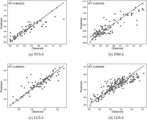
The results show that genetic programming is able to generate formulas with very low mean errors and a good fit to the data. The R² values show how far the predicted values match the observed values. This is more challenging to achieve in large clusters, such as FC5 cluster 5, FB6 cluster 2, LC5 cluster 2, and LC6 cluster 3, which have R² values around 0.80. To better visualize the performance of GP, the observed and predicted values for these clusters are illustrated by a set of plots in Figure 3. The diagonal line between the predicted and observed values represents the case where there is an exact match, which is impossible to achieve practically. However, even for larger values, the points are accumulated around this line, which is considered to be challenging for empirical formulas. The plots also reflect the controlled nature of the laboratory experiments, where the data has a more balanced distribution among the values, and where real-life data has accumulated within lower values with a few cases at larger ones.

Figure 3. These plots of large clusters show how similar the predicted values are to the observed values. The $y=x$ diagonal line shows perfect fit to data. The plots show that laboratory observations are more controlled and almost evenly distributed while the field data accumulates at a range between 0 and 2, while having larger values occasionally.

The most significant outcome of these results is that hierarchical clustering make it possible to bring together a large number of similar observations from different studies. Rather than reporting the intervals on several parameters, the clustering process forms more homogeneous data sets which in turn helps to improve R² scores.

Even though the proposed approach appears to prevent generalization by forming several clusters, and running genetic programming on all of them, it can promote generalization of the data, but only in observations that are similar. Since these data sets have measurements from different environments and setups, the parameters are unable to capture all of the forces acting on a local scour. Therefore, clustering helps bring together similar observations where it is impossible to conduct manual or visual separation in five or six dimensions. Table 8 lists the centers for each cluster. The centers for the clusters within a data set have distinct values, bringing together similar observations, and therefore improving the scour depth prediction.

Table 8. The centers of the clusters after hierarchical clustering

Data Set	Cluster No	${\sigma }_g$	$F_r$	$R_e$	$y/b$	$u/u_c$	$b/D_{50}$
FC5	1		0.22523	9460.9	0.93748	0.76859	840.37
	2		0.43685	101600	1.3305	0.72798	63.334
	3		0.39784	82812	2.0848	0.85888	155.98
	4		0.26706	50300	3.5868	0.57963	187.46
	5		0.12023	18350	2.8768	0.35992	569.81
	6		0.25666	6881.5	0.86875	0.86132	453.31
FC6	1	2.088	0.086631	5487.4	4.8355	0.76803	1134.4
	2	2.0313	0.1758	33514	4.7772	0.56	599.14
	3	4.495	0.19933	22775	1.1289	0.52884	2172.9
	4	0.66437	0.32738	15149	0.84542	0.76955	361.14
FB5	1		0.18635	699.28	1.001	2.1132	44797
	2		0.23587	2917.1	1.1627	1.2118	936.14
	3		0.45762	41529	0.99893	1.6898	2338.6
	4		0.3796	41685	2.1273	1.196	356.82
	5		0.14767	730.46	5.1409	1.8741	1381.9
	6		0.34404	710.79	1.6204	5.853	14416
	7		0.18932	861.14	5.8938	3.8194	6617.9
	8		0.16381	659.78	2.3986	2.045	9951.1
FB6	1	0	0.22107	1247	1.0164	2.4522	18002
	2	2.6317	0.16538	1203.6	4.2282	1.8365	1807.4
	3	0.20432	0.41924	8624.2	0.48098	1.9522	3285.3
LC5	1		0.14475	205.95	4.1297	0.73695	157.23
	2		0.19582	230.61	2.0522	0.71364	132.87
	3		0.27564	191.53	0.68275	0.78205	269.4
LC6	1	1.2557	521.34	923.42	1.3144	0.6365	61.063
	2	1.2618	298.05	438.91	2.8188	0.56056	40.873
	3	1.3749	106.99	204.69	2.4483	0.72297	202.75
LB5	1		0.54032	1056.3	1.2347	1.3139	312.3
	2		0.81302	717.62	1.7719	3.0048	283.25
	3		0.46511	594.87	4.5693	1.7203	78.192
LB6	1	1.2881	0.51422	310.19	2.679	2.1087	173.97
	2	1.591	0.51357	765.73	3.8135	1.5889	53.494

Depending on the category of the data, the closest Euclidean distance between the data and the cluster center determines the formula to be used. For the resulting 32 clusters, there are 32 formulas, most of them very large. Instead of reporting them here, the formulas are made available online at http://homes.ieu.edu.tr/koguz/research/scour/ with a simple user interface that finds the closest cluster and predicts the scour depth $d_s$ using the formula of that cluster, as mentioned earlier.

For a comparison of our results and existing empirical solutions, the three most commonly used formulas are tested with the data. The HEC-18 is also known as the Colorado State University equation (Richardson and Davis 2001), and defined by the formula in Equation 10(10) $\frac{{\mathrm{d}}_{\mathrm{s}}}{\mathrm{b}}=2.0K_1{K}_2{K}_3{K}_4{\left(\frac{y}{b}\right)}^{0.35}{F}_r^{0.43}$(10) where $K_1$ is the correction factor for pier nose shape; $K_2$ is the correction factor for angle of attack of flow;$K_3$ is the correction factor for bed condition; $K_4$ is the correction factor for armoring by bed material size and $F_r$ is the Froude Number directly upstream of the pier.

(10) $\frac{{\mathrm{d}}_{\mathrm{s}}}{\mathrm{b}}=2.0K_1{K}_2{K}_3{K}_4{\left(\frac{y}{b}\right)}^{0.35}{F}_r^{0.43}$(10)

The second empirical formula is by Melville (Melville 1997) as given in Equation 11(11) ${\mathrm{d}}_{\mathrm{s}}=K_{yb}{K}_I{K}_d{K}_s{K}_{\mathrm{\Theta }}{K}_G$(11) . In this formula $K_{yb}$ is the depth size for piers; $K_I$ is the flow intensity; $K_d$ is the sediment size; $K_s$ is the pier shape coefficient; $K_{\mathrm{\Theta }}$ is the pier alignment and $K_G$ is the channel geometry.

(11) ${\mathrm{d}}_{\mathrm{s}}=K_{yb}{K}_I{K}_d{K}_s{K}_{\mathrm{\Theta }}{K}_G$(11)

The third formula is by Jain and Fischer as given in Equation 12(12) $\begin{array}{ccc}\frac{d_{s1}}{b}=2.0{(F_r-F_{rc})}^{0.25}{\left(\frac{y}{b}\right)}^{0.5},& for\left(F_r-F_{rc}\right)\ge 0.2,& \mathrm{l}\mathrm{i}\mathrm{v}\mathrm{e}-\mathrm{b}\mathrm{e}\mathrm{d}\mathrm{s}\mathrm{c}\mathrm{o}\mathrm{u}\mathrm{r}\\ \frac{d_{s2}}{b}=1.85F_{rc}^{0.25}{\left(\frac{y}{b}\right)}^{0.3},& for\left(F_r-F_{rc}\right)\le 0,& \mathrm{c}\mathrm{l}\mathrm{e}\mathrm{a}\mathrm{r}-\mathrm{w}\mathrm{a}\mathrm{t}\mathrm{e}\mathrm{r}\mathrm{s}\mathrm{c}\mathrm{o}\mathrm{u}\mathrm{r}\\ \frac{d_s}{b}=max\left(d_{s1},d_{s2}\right),& for0<\left(F_r-F_{rc}\right)<0.2& \hspace{0.17em}\\ \hspace{0.17em}& & \end{array}$(12) where they provide different formulas for the cases that involve the critical Froude Number $F_{rc}$ defined as $F_{rc}=u_c/\sqrt{gy}$ (Jain and Fischer 1979).

(12) $\begin{array}{ccc}\frac{d_{s1}}{b}=2.0{(F_r-F_{rc})}^{0.25}{\left(\frac{y}{b}\right)}^{0.5},& for\left(F_r-F_{rc}\right)\ge 0.2,& \mathrm{l}\mathrm{i}\mathrm{v}\mathrm{e}-\mathrm{b}\mathrm{e}\mathrm{d}\mathrm{s}\mathrm{c}\mathrm{o}\mathrm{u}\mathrm{r}\\ \frac{d_{s2}}{b}=1.85F_{rc}^{0.25}{\left(\frac{y}{b}\right)}^{0.3},& for\left(F_r-F_{rc}\right)\le 0,& \mathrm{c}\mathrm{l}\mathrm{e}\mathrm{a}\mathrm{r}-\mathrm{w}\mathrm{a}\mathrm{t}\mathrm{e}\mathrm{r}\mathrm{s}\mathrm{c}\mathrm{o}\mathrm{u}\mathrm{r}\\ \frac{d_s}{b}=max\left(d_{s1},d_{s2}\right),& for0<\left(F_r-F_{rc}\right)<0.2& \hspace{0.17em}\\ \hspace{0.17em}& & \end{array}$(12)

These empirical formulas are run on the observations of each of the clusters that are formed by the proposed method. The R² results are given in Table 9 alongside the scores of the results generated by genetic programming.

Table 9. The performance comparison of our method with formulas HEC-18 (Richardson and Davis 2001), Melville (Melville 1997), Jain and Fischer (Jain and Fischer 1979)

Data Set	Cluster No	HEC-18	Melville	Jain and Fischer	This Study
FC5	1	0.331507971	0.277580098	0.014565934	0.800275
	2	0.062945935	0.086026014	0.106400447	0.886301
	3	0.3497482	0.243307859	0.158143031	0.818108
	4	0.082890735	0.00319219	0.029988405	0.800042
	5	0.294976311	0.290508087	0.011480782	0.804223
	6	0.157357114	0.014570134	0.303799706	0.800589
FC6	1	0.191933014	0.271378606	0.100487313	0.829914
	2	0.090716458	0.012302472	0.023148688	0.800074
	3	0.048153021	0.001489986	0.026724057	0.801273
	4	0.011271844	0.048136217	0.000632862	0.801458
FB5	1	0.003662855	0.00000541	0.063332313	0.805511
	2	0.001912554	0.002051145	0.00875351	0.801219
	3	0.019361782	0.104417575	0.0016195	0.801597
	4	0.000212602	0.027951078	0.128290568	0.840243
	5	0.069550409	0.022266545	0.028556313	0.805651
	6	0.145290394	0.004444581	0.136717185	0.950066
	7	0.129009955	0.020443494	0.09620118	0.803619
	8	0.011322782	0.066984863	0.0000001	0.884063
FB6	1	0.498485523	0.287938708	0.26357265	0.804799
	2	0.027278085	0.009814272	0.280456651	0.800156
	3	0.078048793	0.328535146	0.362830688	0.806265
LC5	1	0.027976806	0.022102936	0.015052039	0.806122
	2	0.22501321	0.074365415	0.144046591	0.800543
	3	0.085320422	0.061751552	0.090877131	0.802268
LC6	1	0.468782091	0.702613603	0.79191282	0.954166
	2	0.191146756	0.454842754	0.145084758	0.906428
	3	0.029543504	0.146357597	0.097010229	0.800005
LB5	1	0.14901361	0.254375712	0.546943456	0.807244
	2	0.380280717	0.263218018	0.413500722	0.837667
	3	0.001834544	0.013692274	0.003130038	0.802954
LB6	1	0.614636767	0.398204689	0.640002654	0.8101
	2	0.029094086	0.026969666	0.008632601	0.801582

Table 9 shows generally poor performance of the empirical formulas compared to the formulas generated by GP. It is apparent that it is impossible to obtain a single formula to predict the scour depth in all of these cases without understanding the contribution to the problem of each parameter, including those yet to be identified.

Another analysis that can be performed is the effect of having 5-tuples or 6-tuples for scour depth prediction. Collecting measurements is challenging, therefore further analysis is required to discover whether the prediction with 5-tuples is as good as that with 6-tuples. Since we cannot add ${\sigma }_g$ values to 5-tuples, we use 6-tuple data sets and compare the R² values for these using their variables other than ${\sigma }_g$. Table 10 lists the results when ${\sigma }_g$ is removed from 6-tuple sets. In the majority of the data sets, removing ${\sigma }_g$ resulted in lowered R² values, especially for larger data sets. The variable the geometric standard deviation of the particle size distribution ${\sigma }_g$ shows uniformity of the sediment particles and if ${\sigma }_g>1.3$ the sediment particles can be considered as uniform. In case of ${\sigma }_g>1.3$, armoring occurs on the channel bed and in the scour hole around the pier (Melville 1997). We hypothesize that varying results may be due to the grain distribution curve of sediment particles within the clusters.

Table 10. Comparison of $R^2$ with and without ${\sigma }_g$ parameter for clusters with 6-tuples

Data Set	Cluster No	R^2 for 5-tuple	R^2 for 6-tuple
FC6	1	0.8911	0.8413
FC6	2	0.7891	0.8138
FC6	3	0.8711	0.8238
FC6	4	0.7946	0.8596
FB6	1	0.9023	0.8199
FB6	2	0.8019	0.8207
FB6	3	0.9254	0.8971
LC6	1	N/A	0.9551
LC6	2	0.9311	0.9222
LC6	3	0.8503	0.8132
LB6	1	0.6736	0.8370
LB6	2	0.1221	0.8315

Conclusion

In this study, a new approach to scour depth prediction is proposed. All the available data in the literature were collected and they are grouped by hierarchical clustering to find the real classes in them. For each cluster genetic programming was used to evolve formulas that operate with constants, variables, measured data, and modified mathematical functions.

The results show that when GP is performed on clusters that contain similar observations, the mean errors decrease and the predicted values become more correlated to the observed values. When compared with the existing empirical formulas, better results are implied for formulas tailored to specific classes compared to a single general formula for all cases. The existing formulas were only successful in a few clusters, possibly those similar to the data they were developed for.

A JavaScript application is made available to find the closest cluster and to apply the formula for that cluster. The cluster centers and formulas specific to each cluster are also listed in the source code of this application. The client-based application works online, which makes the results of this study generally available. The application could be used to predict the scour depth when the relevant parameters are provided.

While the application provides access to the results of this study, it should be noted that these formulas were evolved from previously existing data. As mentioned earlier, some measurements not sufficiently close to any cluster center have been removed as outliers; however, as new observations become available, these outliers could form new clusters. Therefore, the process should be repeated to allow new formulas to be evolved in the future. However, this does not alter the strength of the proposed approach. Grouping similar observations from different studies increases the sample size, and provide better generalization within the cluster itself.

Acknowledgments

We thank the anonymous reviewers for their valuable comments and feedback which have improved the manuscript significantly. We are grateful for the high-end system Assoc. Prof. Dr. Osman Doluca has provided to speed up the training of our data. We are also indebted to Simon Edward Mumford for his help in language editing and proofreading.

Disclosure statement

No potential conflict of interest was reported by the author(s).

Correction Statement

This article has been republished with minor changes. These changes do not impact the academic content of the article.

References

- Aksoy, A. Ö., G. Bombar, T. Arkı¸s, and M. S. ¸. Guney. 2017. Study of the time-dependent clear water scour around circular bridge piers. Journal of Hydrology and Hydromechanics (Berlin) 65 (1):1–26. doi:10.1515/johh-2016-0048.
- Alpaydın, E. 2020. Introduction to Machine Learning. 4th ed. Cambridge, Massachusetts: The MIT Press.
- Azamathulla, H. M., A. Ab Ghani, N. A. Zakaria, and A. Guven. 2010. Genetic programming to predict bridge pier scour. Journal of Hydraulic Engineering 136 (3):165–69. doi:10.1061/(ASCE)HY.1943-7900.0000133.
- Azmathullah, H. M., M. C. Deo, and P. B. Deolalikar. 2005. Neural networks for estimation of scour downstream of a ski-jump bucket. Journal of Hydraulic Engineering 131 (10):898–908. doi:10.1061/(ASCE)0733-9429(2005)131:10(898).
- Bata, G., and V. Todorovic. 1960. Erozija iko novosadskog mostovskog stuba (Scour around bridge piers - Novi Sad):Institut za vodoprivredu. Jaroslav Cerni, Beograd, Yugoslavia 59–66.
- Bateni, S. M., S. M. Borghei, and D.-S. Jeng. 2007. Neural network and neuro-fuzzy assessments for scour depth around bridge piers. Engineering Applications of Artificial Intelligence 20 (3):401–14. doi:10.1016/j.engappai.2006.06.012.
- Benedict, S. T., and A. W. Caldwell. 2006. Development and evaluation of clear-water pier and contraction scour envelope curves in the Coastal Plain and Piedmont Provinces of South Carolina. Report 2005–5289, U.S. Geological Survey Scientific Investigations. p.98. http://pubs.usgs.gov/sir/2005/5289.
- Benedict, S., and W. Caldwell. 2009. Development and evaluation of live-bed pier and contraction scour envelope curves in the Coastal Plain and Piedmont Provinces of South Carolina. Report 2009–5099, U.S. Geological Survey Scientific Investigations. p.108. http://pubs.usgs.gov/sir/2009/5099/
- Boehmler, E. M., and J. R. Olimpio. 2000. Evaluation of pier scour measurement methods and pier- scour predictions with observed scour measurements at selected bridge sites in New Hampshire, 1995–98: Report 00–4186, p. 58, p.108. U.S. Geological Survey Scientific Investigations.
- Bor, A. 2015. Experimental and numerical study of local scour around bridge piers with different cross sections caused by flood hydrograph succeeding steady flow.” PhD diss., Phd Thesis, Dokuz Eylül University, Ankara.
- Breusers, H. N. C., G. Nicollet, and H. W. Shen. 1977. Local scour around cylindrical piers. Journal of Hydraulic Research 15 (3):211–52. doi:10.1080/00221687709499645.
- Butch, G. K. 1991. Measurement of bridge scour at selected sites in New York, excluding Long Island. Report 91–4083 21. U.S. Geological Survey Water-Resources Investigations.
- Chabert, J., and P. Engeldinger. 1956. Etude des affouillements autour des piles de ponts (Study of scouring around bridge piers). France: Chatou, France: Laboratoire National d’Hydraulique.
- Chang, F. M. 1980. Scour at bridge piers; field data from Louisiana files: Report FHWA-RD-79-105. As cited in Froehlich (1988), Federal Highway Administration.
- Chee, R. K. W. 1982. Live-bed scour at bridge piers. Report No. 290. As cited in Sheppard and others (2011). Auckland, New Zealand: The University of Auckland, School of Engineering.
- Cheong, S.-U. C. S. 2006. Prediction of local scour around bridge piers using artificial neural networks1. JAWRA Journal of the American Water Resources Association 42 (2):487–94. doi:10.1111/j.1752-1688.2006.tb03852.x.
- Chicco, D., M. J. Warrens, and G. Jurman. 2021. The coefficient of determina- tion R-squared is more informative than SMAPE, MAE, MAPE, MSE and RMSE in regres- sion analysis evaluation”[in en]. PeerJ Computer Science 7 (July): e623. Accessed August 22, 2021. doi: 10.7717/peerj-cs.623.
- Chiew, Y.-M. 1984. Local scour at bridge piers. Report No. 355. As cited in Sheppard and others (2011), Auckland, New Zealand: The University of Auckland, School of Engineering.
- Choi, S.-U., B. Choi, and S. Lee. 2017. Prediction of local scour around bridge piers using the ANFIS method. Neural Computing and Applications 28(2): 335–44. (February). Accessed March 29, 2020. doi:10.1007/s00521-015-2062–1.
- Coleman, S. E., C. S. Lauchlan, and B. W. Melville. 2003. Clear-water scour development at bridge abutments. Journal of Hydraulic Research 41 (5):521–31. doi:10.1080/00221680309499997.
- Dabhi, V. K., and C. Sanjay. 2015a. Empirical modeling using genetic programming: A survey of issues and approaches. Natural Computing 14(2): 303–30. June. 1572–9796. doi:10.1007/s11047-014-9416-y.
- Dabhi, V. K., and C. Sanjay. 2015b. Empirical modeling using genetic programming: A survey of issues and approaches. Natural Computing 14(2): 303–30. (June). Accessed August 22, 2021. doi:10.1007/s11047-014-9416-y.
- Dang, N. M., D. T. Anh, and T. D. Dang. 2019. ANN optimized by PSO and Firefly algorithms for predicting scour depths around bridge piers. Engineering with Computers (July). Accessed November 29, 2020. doi:10.1007/s00366-019-00824–y.
- Davoren, A. 1985. Local scour around a cylindrical bridge pier:Publication no. 3. Technical report. As cited in Froehlich (1988), Christchurch, New Zealand: Hydrology Center.
- Dey, S., and R. V. Raikar. 2005. Scour in long contractions. Journal of Hydraulic Engineering 131 (12):1036–49. doi:10.1061/(ASCE)0733-9429(2005)131:12(1036).
- Dey, S., S. K. Bose, and G. L. N. Sastry. 1995. Clear water scour at circular piers-A model. Journal of Hydraulic Engineering, American Society of Civil Engineering 121 (12):869–76. doi:10.1061/(ASCE)0733-9429(1995)121:12(869).
- Ettema, R. 1976. Influence of bed material gradation on local scour. Report No. 124. As cited in Sheppard and others (2011), Auckland, New Zealand: The University of Auckland, School of Engineering.
- Ettema, R. 1980. “Scour at bridge piers.” PhD diss., Phd Thesis, University of Auckland, Auckland.
- Ettema, R., G. Kirkil, and M. Muste. 2006, January 1. Similitude of large-scale turbulence in experiments on local scour at cylinders. Journal of Hydraulic Engineering 132 (1):33–40. https://doi.org/10.1061/(ASCE)0733-9429(2006)132:1(33)
- Firat, M., and M. Gungor. 2009. Generalized regression neural networks and feed forward neural networks for prediction of scour depth around bridge piers. Advances in Engineering Software 40 (8):731–37. doi:10.1016/j.advengsoft.2008.12.001.
- Fortin, F.-A., F.-M. De Rainville, M.-A. Gardner, M. Parizeau, and C. Gagné. 2012. DEAP: Evolutionary algorithms made easy. Journal of Machine Learning Research 13 (July):2171–75.
- Gao, D., L. Posada, and C. F. Nordin. 1993. Pier scour equations used in the People’s Republic of China. Report FHWA-SA-93-076. As cited in Sheppard and others (2011). Wash- ington, DC, Federal Highway Administration.
- Graf, W. H. 1995. Load scour around piers. Annual Report p. B.33.1-B.33.8. As cited in Sheppard and others (2011), Lausanne, Switzerland, Laboratoire de Recherches Hydrauliques: Ecole Polytechnique Federale de Lausanne.
- Guven, A., H. M. Azamathulla, and N. A. Zakaria. 2009. Linear genetic programming for prediction of circular pile scour. Ocean Engineering 36 (12):985–91. doi:10.1016/j.oceaneng.2009.05.010.
- Hager, W. H., and J. Unger. 2010. Bridge Pier Scour under flood waves. Journal of Hydraulic Engineering 136 (10):842–47. doi:10.1061/(ASCE)HY.1943-7900.0000281.
- Hayes, D. C. 1996. Scour at bridge sites in Delaware, Maryland, and Virginia. Report 96–4089, U.S. Geological Survey Water-Resources Investigations. 39.
- Hodgkins, G., and P. Lombard. 2002. Observed and prediction pier scour in Maine. Report 02–4229, U.S. Geological Survey Water-Resources Investigations. 30p.
- Hoffmans, G. J. C. M., and H. J. Verheij. 1997. Scour Manual. Rotterdam: A.A. Balkema: A.A. Balkema Publishers.
- Holnbeck, S. R. 2011. Investigation pier scour in coarse-bed streams in Montana, 2001 through 2007. Report 2011–5107, U.S. Geological Survey Scientific Investigations. 68.
- Hopkins, G. R., R. W. Vance, and B. Kasraie. 1980. Scour around bridge piers. Report FHWA- RD-79-103, 131. Federal Highway Administration.
- Jain, S. C., and E. E. Fischer. 1979. Scour around bridge piers at high Froude numbers. FHWA- RD-79-104. As cited in Sheppard and others (2011). available from NTIS, 5285 Port Royal Road, Springfield, Virginia 22161, Federal Highway Administration Report.
- Jain, S. K. 2001. Development of integrated sediment rating curves using ANNs. Journal of Hydraulic Engineering 127 (1):30–37. doi:10.1061/(ASCE)0733-9429(2001)127:1(30).
- Jolliffe, I. 2005. Principal component analysis. In Encyclopedia of statistics in behavioral science, 1-6, New York: American Cancer Society. isbn: 9780470013199. doi:10.1002/0470013192.bsa501.
- Kaya, A. 2010. Artificial neural network study of observed pattern of scour depth around bridge piers. Computers and Geotechnics 37 (3):413–18. doi:10.1016/j.compgeo.2009.10.003.
- Lan¸ca, R. M., C. S. Fael, R. J. Maia, J. P. Pêgo, and A. H. Cardoso. 2013. Clear-water scour at comparatively large cylindrical piers. Journal of Hydraulic Engineering 139 (11):1117–25. doi:10.1061/(ASCE)HY.1943-7900.0000788.
- Lee, T. L., D. S. Jeng, G. H. Zhang, and J. H. Hong. 2007. Neural network modeling for estimation of scour depth around bridge piers. Journal of Hydrodynamics, Ser. B 19 (3):378–86. doi:10.1016/S1001-6058(07)60073-0.
- Liriano, S., and R. Day. 2001. Prediction of scour depth at culvert outlets using neural networks. Journal of Hydroinformatics 3 (4):231–38. doi:10.2166/hydro.2001.0021.
- Max, S. D., M. Odeh, and T. Glasser. 2004. Large scale clear-water local pier scour experiments. Journal of Hydraulic Engineering 130 (10):957–63. doi:10.1061/(ASCE)0733-9429(2004)130:10(957).
- Max, S. D., and W. Miller Jr. 2006. Live-bed local pier scour experiments. Journal of Hydraulic Engineering 132 (7):635–42. doi:10.1061/(ASCE)0733-9429(2006)132:7(635).
- Melville, B. W. 1975. Local scour at bridge sites PhD diss., Auckland: University of Auckland, School of Engineering.
- Melville, B. W., and Y.-M. Chiew. 1999. Time scale for local scour at bridge piers. Journal of Hydraulic Engineering 125 (1):59–65. doi:10.1061/(ASCE)0733-9429(1999)125:1(59).
- Melville, B. W. 1997. Pier and Abutment Scour: Integrated Approach. Journal of Hydraulic Engineering 123 (2):125–36. doi:10.1061/(ASCE)0733-9429(1997)123:2(125).
- Mignosa, P. 1980. Fenomeni di Erosione Locale alla Base delle Pile del Ponti PhD diss., Tesi di LAura, Department of Hydraulics Structure, Politecnico di Mlano, Milan, Italy.
- Mohammadpour, R., A. A. B. Ghani, and H. M. Azamathulla. 2013. Estimation of dimension and time variation of local scour at short abutment. International Journal of River Basin Management 11 (1):121–35. doi:10.1080/15715124.2013.772522.
- Muller, D. S., and C. R. Wagner. 2005. Field observations and evaluations of streambed scour at bridges. Technical report, McLean, Virginia: Office of Engineering Research and Development, Federal Highway Administration.
- Muller, D. S., R. L. Miller, and J. T. Wilson. 1994. Historical and potential scour around bridge piers and abutments of selected stream crossing in Indiana. Report 93–4066, p.123. U.S. Geological Survey Water-Resources Investigations.
- Najafzadeh, M., and G.-A. Barani. 2011. Comparison of group method of data handling based genetic programming and back propagation systems to predict scour depth around bridge piers. Scientia Iranica 18 (6):1207–13. doi:10.1016/j.scient.2011.11.017.
- Neil, C. R. 1965. Measurements of bridge scour and bed changes in a flooding sand-bed river. Proceedings of the Institution of Civil Engineers, 30(2), 415–435. London, England: The Institution of Civil Engineers.
- Oliveto, G., and W. H. Hager. 2002. Temporal evolution of clear-water pier and abutment scour. Journal of Hydraulic Engineering 128 (9):811–20. doi:10.1061/(ASCE)0733-9429(2002)128:9(811).
- Pal, M., N. K. Singh, and N. K. Tiwari. 2011. Support vector regression based modeling of pier scour using field data. Engineering Applications of Artificial Intelligence 24 (5):911–16. doi:10.1016/j.engappai.2010.11.002.
- Pal, M. 2019. Deep neural network based pier scour modeling. ISH Journal of Hydraulic Engineering:1–6. doi:10.1080/09715010.2019.1679673.
- Pandey, M. P., K. Sharma, Z. Ahmad, U. K. Singh, and N. Karna. 2018. Three- dimensional velocity measurements around bridge piers in gravel bed. Marine Georesources & Geotechnology 36 (6):663–76. doi:10.1080/1064119X.2017.1362085.
- Pandey, M., S.-C. Chen, P. K. Sharma, C. S. P. Ojha, and V. Kumar. 2019. Local scour of armor layer processes around the circular pier in non-uniform gravel bed. Water 11 (7):1421. 2073–4441. doi:10.3390/w11071421.
- Pizarro, A., S. Manfreda, and E. Tubaldi. 2020. The science behind scour at bridge foundations: A review. Water 12 (2): 374. (February). Accessed March 29, 2020. doi:10.3390/w12020374.
- Poli, R., W. B. Langdon, N. F. McPhee, and J. R. Koza. 2008. A field guide to genetic programming. United Kingdom: Lulu Enterprises, UK Ltd.
- Richardson, E. V., and S. R. Davis. 2001. Evaluating scour at bridges. Report. Number FHWA NHI 01–001. Washington, D.C.: Federal Highway Administration.
- Sharafati, A., M. Haghbin, D. Motta, and Z. M. Yaseen. 2019. The application of soft computing models and empirical formulations for hydraulic structure scouring depth simulation: A comprehensive review, assessment and possible future research direction. Archives of Computational Methods in Engineering November. 1886–1784. Accessed March 29, 2020. doi:10.1007/s11831-019-09382-4.
- Shen, H. W. 1975. Compilation of scour data based on California bridge failures. Publication FHWA-RD-76-142, 28. Department of Transportation Federal Highway Administration.
- Shen, H. W., V. R. Schneider, and S. Karaki. 1969. Local scour around bridge piers. Journal of the Hydraulics Division 96:HY6.
- Sheppard, D. M., B. W. Melville, and H. Demir. 2014. Evaluation of existing equations for local scour at bridge piers. Journal of Hydraulic Engineering 140 (1):14–23. doi:10.1061/(ASCE)HY.1943-7900.0000800.
- Southard, S. E. 1992. Scour around bridge piers on stream bank in Arkansas. Report 92–4126, 29. U.S. Geological Survey Water-Resources Investigations.
- Trent, R., N. Gagarin, and J. Rhodes. 1993. Estimating pier scour with artificial neural networks. In Hydraulic engineering, 1043–48. USA: ASCE.
- USGeologicalSurvey. 2001. National bridge scour database. USGS. Accessed April 15, 2014. http://water.usgs.gov/osw/techniques/bs/BSDMS/index.htm
- Vanneschi, L., M. Castelli, and S. Silva. 2010. Measuring bloat, overfitting and functional complexity in genetic programming In Proceedings of the 12th Annual Con- ference on Genetic and Evolutionary Computation, 877–84. GECCO ‘10. Portland, Oregon, USA: Association for Computing Machinery. doi:10.1145/1830483.1830643.
- Vijayasree, B. A., T. I. Eldho, B. S. Mazumder, and N. Ahmad. 2019. Influence of bridge pier shape on flow field and scour geometry. International Journal of River Basin Management 17 (1):109–29. doi:10.1080/15715124.2017.1394315.
- Wang, C., H.-P. Shih, J.-H. Hong, and R. V. Raikar. 2013. Prediction of bridge pier scour using genetic programming. Journal of Marine Science and Technology 21:483–92.
- Williamson, D. 1993. Local scour measurements at bridge piers in Alberta In Proceedings of the 1993 National Conference on Hydraulic Engineering, p. 534–39. New York: American Society of Civil Engineering.
- Wilson, K. V. 1995. Scour at selected bridge sites in Mississippi: Report 94–4241, p. 48. U.S. Geological Survey Water-Resources Investigations.
- Xu, D., and Y. Tian. 2015. A comprehensive survey of clustering algorithms. Annals of Data Science 2(2): 165–93. June. Accessed August 22, 2021. doi:10.1007/s40745-015-0040-1.
- Yanmaz, A. M., and H. D. Altinbilek. 1991. Study of time dependent local scour around bridge piers. Journal of Hydraulic Engineering 117 (10):1247–68. doi:10.1061/(ASCE)0733-9429(1991)117:10(1247).
- Yanmaz, A. M. 2002. Köprü Hidroliği. Ankara: METU Press.
- Yanmaz, A. M. 2006. Temporal variation of clear water scour at cylindrical bridge piers. Canadian Journal of Civil Engineering 33 (8):1098–102. doi:10.1139/l06-054.
- Zhuravlyov, M. M. 1978. New method for estimation of local scour due to bridge piers and its substantiation. Technical report. As cited in Sheppard and others (2011), Moscow, Russia: Transactions, Ministry of Transport Construction, State All Union Scientific Research Institute on Roads.
- Zohuri, B. 2016. Dimensional analysis beyond the Pi theorem. First ed. Switzerland: Springer Publishing Company.