Rail Steel Health Analysis Based on a Novel Genetic Density-based Clustering Technique and Manifold Representation of Acoustic Emission Signals

ABSTRACT

In order to improve the effectiveness of the acoustic emission (AE) technique in rail health monitoring, a novel genetic clustering technique is proposed to categorize data automatically, integrating density-based clustering and t-distributed stochastic neighbor embedding. A primary problem in optimizing density-based clustering is to accommodate noise, for it explicitly computes the noise subset. Thus, the generalized silhouette index is proposed as a profitable objective to properly tackle noise and arbitrary shapes. The proposed method is initially testified in ten benchmark datasets, which manifests a superiority in handling irregular shape datasets and noise interference. Furthermore, the proposed method is applied in real-world AE signals acquired from tensile tests. The clustering results elucidated that it outperforms the comparative methods in categorizing the fused AE features and remains robust with increasing railway noise interference. In conclusion, the proposed method is validated to discover intrinsic groups of AE data and analyze potential rail health stages.

Introduction

In recent years, high-speed railways have undergone a rapid and worldwide development. Meanwhile, the increase in traffic speed, density and loads on modern railways also draws considerable attention to the reliability, maintainability and safety of railways (Alahakoon et al. 2018). Safety statistics from the Federal Railroad Administration and the European Railway Safety Database in 2016 reveal that approximately 30% of the assigned factors for train accidents that occurred during the last decade were rail-related, which encompasses internal rail defects and surface irregularities (Synodinos 2016). Undetected defects generated in rails have an inclination to grow rapidly, which accelerates the deterioration and causes catastrophic consequences such as derailment. Notably, more than 100 rails are broken annually within the European Union since early the century (Olofsson and Nilsson 2002). This situation has instigated the research community to reconsider more efficient schemes for rail health monitoring and the structural integrity assessment.

Among the emerging techniques for rail health monitoring, the acoustic emission (AE) technique has shown strong superiority on the ground of its high sensitivity and dynamic detection without blind regions, which is particularly applicable to the assessment of health stages. AE is a transient elastic wave caused by partial energy released from sudden structural damage inside a material normally during the growth of cracks, fractures and deformation process. During such degradation, multiple failure mechanisms tend to become active and dominant in sequential health stages, resulting in the generation of AE signals with distinctive waveforms and statistical characteristics (Angelopoulos and Papaelias 2018). By evaluating AE signals based on their characteristics, it is possible to categorize them into different stages and improve the effectiveness of the AE technique in structural health monitoring. However, the damage mechanism patterns and conditional probability distributions involved must be known in advance for supervised learning algorithms. Or rather, supervised models often require large amounts of selected training data with external references; however, the prior health information is generally unavailable in the field application. Moreover, it is of significance to ascertain that these man-made labels for health diagnosis are ground-truth and deepen our understanding in practice. Comparatively, the clustering process can reflect the internal structure, and natural patterns of data are effectively extracted using automated clustering algorithms.

The feasibility of various clustering algorithms for AE data clustering has been considered in several studies. In (Yang, Kang, and Zhou 2015), k-means using peak frequency of AE signals as the key parameter is employed to discriminate the failure types of thermal barrier coatings and the optimal number of clusters is determined according to the maximum of the silhouette values. Sibil et al. (2012) presents a genetic algorithm-based method to perform the k-means clustering steps, group AE signals obtained from different materials, and evaluates the performance with the Davies–Bouldin index. Zhang et al. (2020) brought forward a joint optimization between encoder–decoder deep network and k-means to obtain clustering-friendly features. The iterative self-organizing data analysis technique algorithm (ISODATA) attempts to modify the uncertainty of cluster numbers of k-means by cluster-merging and splitting operations, and its effectiveness in clustering AE data has been evaluated with reinforced composite samples (Angelopoulos and Papaelias 2018). Principal component analysis and kernel fuzzy c-means (KFCM) clustering were combined to compress AE data into 3D features and categorize various damage stages in monitored steel fiber-reinforced concrete specimens (Behnia et al. 2019). The hierarchical clustering model (HCM) partitions data by the agglomerative and divisive procedures through creating and analyzing a cluster tree (dendrogram). Saeedifar et al. (2018) compared different standard clustering methods in differentiating interlaminar and intralaminar damages and concluded that the hierarchical model achieves the best performance. As for unsupervised neural networks, Fukui, Sato, and Mizusaki et al. (2010) explored numerous damage events utilizing a self-organizing map (SOM), introducing Kullback–Leibler (KL) divergence as the kernel function for differentiation of crack and collision. However, normal clustering methods have difficulties in handling datasets with complicated silhouettes or outliers.

Exceptionally, density-based clustering typically considers clusters as high-density regions in the feature space and searches for the connected dense regions. Density-based spatial clustering of applications with noise (DBSCAN) has become one of the most popular and cited algorithms in the literature (Galán 2019). DBSCAN relies on a density-based notion, designed to automatically determine the number of clusters, effectively discover clusters of arbitrary shapes and tackle with outliers (Ester et al. 1996). Despite a number of advantages in the clustering task, it also has some flaws that limit its applicability. On the one hand, it is sensitive to two input parameters, ε (radius of neighborhood) and MinPts (the minimum of neighbors for core points), especially when the density of data is non-uniform. On the other hand, DBSCAN normally has difficulties with high-dimensional databases. Therefore, DBSCAN has been extensively explored for these two problems. In order to determine the feasible parameters, fast DBSCAN chooses the turning point value in the k-dist curve (kth nearest neighbor) as ε where the densities get a sharp rise (Liu 2006). Similarly, partitioning DBSCAN was proposed to partition the datasets into several regions, plotting the k-dist graph in each region and finally merging the clusters of regions (Jiang et al. 2011). To reduce the computational cost, a sampling-based DBSCAN marks eight points in certain directions of boundary in the neighborhood,which is only valid in a two-dimensional space (Borah and Bhattacharyya 2004). Inspired by the above works, Gong et al. (2021) improved the fuzzy C-means method with grid density and distance in the analysis of AE signals for the surveillance of road engineering structures. Another variant of density-based clustering, ordering points to identify the clustering structure technique (OPTICS), is also well known with the advantage that it is insensitive to ε and applicable for data with varying density (Schneider and Vlachos 2017). It generates reachability plot by reordering objects to extract clusters as visualized valleys, but the cluster extraction process requires setting additional threshold or alternative tedious operations. Besides, through introducing the fast search of density peaks as the cluster centroids, a new advanced density-based clustering called the Density Peak Clustering (DPC) was proposed by Rodriguez and Laio (2014) and applied in the acoustic emission analysis to monitor the machine health in a subsequent research (Liu et al. 2018). In order to handle the anomalies, some researches further modified DCP into a residual error-based version by replacing the minimum distance of neighboring point with residual error computation when the decision graphs are generated (Parmar et al. 2019b, 2019a). Therefore, DPC became another representative branch of the density-based clustering techniques and it can be viewed as a combination of the density-based idea and centroid-partition clustering, which is also adopted as a comparison method in this study. However, the parameter selection or region query is either achieved manually or with high computing cost, which is still a challenging task to be solved.

In this study, a genetic strategy is introduced into DBSCAN for automatic region queries and convenient categorization of AE signals by clustering validation index (CVI) without external labels. As far as we are aware, no traditional CVI is capable of explicitly evaluating noise objects that are crucial in DBSCAN. Hence, a generalized silhouette index (GSI) is proposed in this paper to handle noise and increase the feasibility of optimal region queries. With the aim of clustering high-dimensional AE data, a local manifold learning method is also brought forward for a feasible health stage estimation to reduce the feature dimension to an appropriate size and enhance the distinguishability of latent representation of burst AE signals in different stages. Finally, merits of the proposed method, compared with others, are analyzed and discussed thoroughly by external clustering indices.

Theoretical Preliminaries

Clustering is a broadly used unsupervised data mining technique that allows similar objects grouped together and dissimilar objects assigned into different categories. Normally, the similarities are measured based on the Euclidean distance in feature space, and a shorter distance indicates more similarity between objects. On the basis of the spatial similarity, density-based clustering partitions the objects in accordance with density change of their neighbors, grouping together the closely packed points. As one of the most representative algorithms in density-based clustering, density-based spatial clustering of applications with noise (DBSCAN) was initially introduced in this section.

Density Based Spatial Clustering of Applications with Noise (DBSCAN)

Given a set of points of interest, DBSCAN starts with a random point. The corresponding point’s neighborhood is retrieved, which is marked as visited and labeled as core points if it contains sufficient neighbors. Otherwise, the point is labeled as noise or border points. Such a rigorous definition of borders guarantees important characteristics that are insensitive to noise and capable of grouping arbitrarily shaped clusters including spherical, linear, elongated and non-convex shapes, etc. All of the above characteristics make it a good candidate for categorizing the AE signals. To introduce our modification methods, some basic definitions should first be elaborated. Provided with a series of input variables or matrices, a dataset C of N d-dimensional samples, a distance function dist defined over d-dimensional vectors, and two input parameters $\epsilon \in R^{+}$ (radius of neighborhood threshold) and $MinPts\in N^{+}$ (minimum number of neighbors for core points), DBSCAN relies on the definitions below:

• Definition 1 (ε-neighborhood): The ε (Eps)-neighborhood of a point $o_i\in \mathbf{C}$, denoted as $N_{\epsilon }\left(o_i\right)$, is defined by $N_{\epsilon }\left(o_i\right)=\left\{o_j\in \mathbf{C}\left|dist\left(o_i,o_j\right)\le \epsilon \right.\right\}$.

• Definition 2 (Directly density-reachable): $o_i$ is a core point if $\left|N_{\epsilon }\left(o_i\right)\right|\ge MinPts$ where $\left|N_{\epsilon }\left(o_i\right)\right|$ denotes the number of objects in $N_{\epsilon }\left(o_i\right)$. An object $o_j$ is directly density-reachable from $o_i$ if $o_j\in N_{\epsilon }\left(o_i\right)$.

• Definition 3 (Density-reachable): A point $o_j$ is density-reachable from the point $o_i$ if there is a sequence path of z object $\left\{o_1,\dots ,o_k,\dots ,o_z\right\}$, with $o_1=o_i$, $o_z=o_j$ on condition that $o_{k+1}\in \mathbf{C}$ is directly density-reachable from $o_k\in \mathbf{C}$.

• Definition 4 (Density-connected): An object $o_i$ is density-connected to an object $o_j$ if both $o_i$ and $o_j$ are density-reachable from $o_k\in \mathbf{C}$.

• Definition 5 (Cluster): A density-based cluster ${\mathbf{C}}_{ClusterID}$ is a non-empty subset of $\mathbf{C}$ satisfying conditions: (1) $\mathrm{\forall }{o}_i\in {\mathbf{C}}_{ClusterID}$ and $o_j\in \mathbf{C}$, if $o_j$ is density-reachable form $o_i$ then $o_j\in {\mathbf{C}}_{ClusterID}$; and (2) $\mathrm{\forall }{o}_i,o_j\in {\mathbf{C}}_{ClusterID}$, $o_i$ is density-connected to $o_j$.

• Definition 6 (Noise): Let $\left\{{\mathbf{C}}_1,\dots ,{\mathbf{C}}_k\right\}$ be all the clusters in C. The noise ${\mathbf{N}}_n$ is the set of points in C not belonging to any cluster, ${\mathbf{N}}_n=\mathbf{C}-\left\{{\mathbf{C}}_1,\dots ,{\mathbf{C}}_k\right\}$.

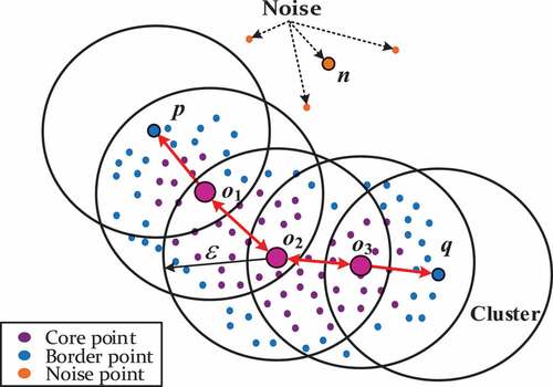
In order to make the definitions more intuitive, the illustrative diagram of DBSCAN is shown in Figure 1. As Figure 1 depicts, p, q, o₁, o₂ and o₃ belong to the same cluster, while point n is a noise point. The red arrows indicate the density-reachable relations. o₁ and o₃ are directly density-reachable from o₂, while p is directly density-reachable from o₁ and q is directly density-reachable from o₃. p and q are thus density-connected by o₂.

Figure 1. Illustrative diagram of the definitions in DBSCAN.

From the view of DBSCAN, every point in the dataset will rigorously fall into either core or non-core points and connectivity to core points will separate outliers and border points. To retrieve all the neighbors of points in dataset C efficiently, a distance matrix $\mathrm{\Delta }={\left\{{\delta }_{ij}\right\}}_{N\times N}$ is generally used, where ${\delta }_{ij}=dist\left(o_i,o_j\right)$, $o_i,o_j\in \mathbf{C}$ and $1\le i,j\le N,i\ne j$.

On the basis of the definitions, the flowchart of DBSCAN algorithm is shown in Figure 2. As the flow chart shows, two global parameters, ε and MinPts, are assumed to be known beforehand and DBSCAN is quite sensitive to the fine-tuning of these two global parameters. In the following section, a heuristic region query process is introduced into DBSCAN to solve this problem by automatic optimization.

Figure 2. Flow chart of DBSCAN algorithm.

Feature Fusion with T-distributed Stochastic Neighbor Embedding

In practice, datasets normally contain a large number of features that cannot guarantee clustering performance. Some can even degrade it by making it computationally inefficient. Empirically, DBSCAN cannot work well with high-dimensional features in view of the curse of dimensionality. In this regard, feature fusion by manifold learning is more effective and reliable than artificial selection. Also, it is beneficial to reduce the computational cost and map the AE datasets into a low-dimensional latent feature space. Fused features not only mirror a better representation of the inherent structure but also alleviate the instability and ill-posed conditions of raw features. T-distributed stochastic neighbor embedding (t-SNE) is envisaged as a novel local manifold learning method (Maaten and Hinton 2008). It maps the points into lower-dimensional manifold by minimizing the Kullback–Leibler divergence. Moreover, it captures most of structural information and retains neighbor similarities of the original data largely intact based on their conditional probability.

Without loss of generality, the raw extracted AE features, $X_N=\left[x_1,x_2,\dots ,x_N\right]$, are assumed to be composed of d₀-dimensional vectors (d₀ ≥ 2) from N objects. To represent high-dimensional data in a d-dimensional feature subspace, $F_N=\left[f_1,f_2,\dots ,f_N\right]$, $d<d_0$, t-SNE converts Euclidean distances between data points into probabilities of similarities. The conditional probability $p_{j\left|i\right.}$ that $x_i$ would pick $x_j$ as its neighbor is calculated as

(1) $p_{j\left|i\right.}=\frac{exp\left(-{∥x_i-x_j∥}^2/2{\sigma }^2\right)}{{\sum }_{k\ne i}exp\left(-{∥x_i-x_k∥}^2/2{\sigma }^2\right)}$(1)

where $\sigma$ is the variance of the Gaussian kernel. In implementation, the estimate of $\sigma$ in $p_{j\left|i\right.}$ is controlled by an entropy-based parameter named perplexity, Perp, which can be viewed as a smooth estimate for a number of neighbors and used to measure local similarities in high dimensional space with an empirical robust range in [5, 100]. The symmetrical joint probability $p_{ij}$ is defined as $p_{ij}=\left(p_{i\left|j\right.}+p_{j\left|i\right.}\right)/2N$. Similarly, a student t-distribution is employed as the heavy-tailed distribution in the low-dimensional manifold, and the neighbor similarities between $f_i$ and $f_j$ can be modeled as

(2) $q_{ij}=\frac{{\left(1+{∥f_i-f_j∥}^2\right)}^{-1}}{{\sum }_{k\ne i}{\left(1+{∥f_i-f_j∥}^2\right)}^{-1}}$(2)

In the ideal case, there exists $p_{ij}=q_{ij}$, indicating that all relative positional relationships between high-dimensional data points have been reserved in subspace. Therefore, the cost function of Kullback–Leibler divergence (KL divergence) is applied to obtain the latent feature by assessing the proximity between $p_{ij}$ and $q_{ij}$.

(3) $KL\left(P∥Q\right)=\sum _i\sum _j{p}_{ij}log\frac{p_{ij}}{q_{ij}}$(3)

Region Query of Clustering with Genetic Algorithm

In order to improve the clustering efficiency, this paper combines an optimization algorithm with density-based clustering and t-SNE to stabilize the region query process with a cluster validation index (CVI). Note that there is no explicit expression for CVIs in DBSCAN and it cannot be obtained through gradient descent methods. Fortunately, the genetic algorithm (GA) is a meta-heuristic search algorithm and one predominant potential of GA is that it compares objective functions from parallel solutions rather than updating directly toward the derivative. The objective function in GA, also called a fitness function, can be non-differentiable or truly opaque.

In genetic algorithms, the solution region is normally binary encoded in the form of gene strings named chromosomes. Each chromosome represents an individual corresponding to a unique candidate solution, the group of which is a population. Both crossover and mutation operators produce diverse offspring, ensuring sufficient exploration of the global optimum. Through external survival pressure imposed by the fitness function, genetic traits evolve to optimal solutions over several generations. The details of GA implementation are elaborated as follows:

1. In this experiment, each generation consists of 20 chromosomes. For continuous variables like ε, generating a chromosome section of 25 bits and the highest optimization accuracy of $1\times {10}^{-7}$ can be achieved. For the other integer variable, a section of 7 bits is assigned to cover the span of [1,100]. Selective parent reproduction is performed by roulette wheel selection.

2. A uniform crossover is applied and the crossover rate is set to 0.7. Crossover points in parent chromosomes are randomly selected and swapped at crossover points to produce two new offsprings.

3. The mutation operator randomly changes a gene value of an offspring to create a new chromosome. Each chromosome undergoes mutation with a probability of 0.02.

4. Once a new population is generated, each chromosome is decoded by converting bit string into actual values. The generated population is evaluated by fitness values and the region query is executed, ranking of chromosomes. The maximum of iterative generations is set as 50. In order to obtain the optimal categorization, the internal clustering validation index (CVI) should be investigated first.

Generalized Silhouette Index

Internal clustering validation indices generally evaluate the goodness of clustering structure without reference to additional information and are vital in practical scenarios without available ground-truth data. Internal CVI contains two parts: within-cluster compactness and the between-cluster separability. They are indispensable properties for an intuitively acceptable cluster concept. Literatures indicate that the silhouette index (SI) has performed well in most comparative experiments (Amorim and Hennig 2015). The silhouette width for the ith object, s(x_i), validates the clustering performance of a single object based on the pairwise difference of separability b(i) and compactness a(i) as follows:

(4) $\left\{\begin{array}{c}b\left(i\right)=\underset{1\le j\le N_C,j\ne l}{min}\left\{\frac{1}{n_j}\sum _{p=1}^{n_j}dist\left(x_i^{\left(l\right)},x_p^{\left(j\right)}\right)\right\}\\ a\left(i\right)=\frac{1}{n_l-1}\sum _{q=1,q\ne i}^{n_l}dist\left(x_i^{\left(l\right)},x_q^{\left(l\right)}\right)\end{array}\right.$(4)

where N and N_C are the total number of samples and clusters; the ith sample, $x_i^{\left(l\right)}$ belongs to the lth cluster ${\mathbf{C}}_l\in \mathbf{C}$ with n_l samples; and b(i) and a(i) are measured by between- and within-cluster dissimilarity. All the mentioned dissimilarities are measured in the Euclidean distance. Then, the silhouette index of C is defined as the average silhouette width:

(5) $SI\left(\mathbf{C}\right)=\frac{1}{N}\sum _{l=1}^{N_C}\sum _{x_i\in {\mathbf{C}}_l}s\left(x_i\right)=\frac{1}{N}\sum _{l=1}^{N_C}\sum _{x_i\in {\mathbf{C}}_l}\left[\frac{b\left(i\right)-a\left(i\right)}{max\left\{a\left(i\right),b\left(i\right)\right\}}\right]$(5)

Normally, the silhouette index ranges from 1, indicating that points are distant from neighboring clusters, to −1, indicating incorrect clustering. However, like most CVIs, SI does not have a rigorous rule to tackle noise, which is intrinsic in density clustering because it explicitly computes outliers (Liu et al. 2013; Valdes, Cheung, and Rubio 2017). Without intervention, SI would embed the outliers as an additional group. Therefore, the silhouette index is modified into a novel version, generalized silhouette index (GSI), which is capable of handling noise and applicable in the region query of DBSCAN. We assume that the dataset of N objects is partitioned by a clustering solution $\mathbf{C}=\left(\left\{{\mathbf{C}}_l\right\}\cap {\mathbf{N}}_n\right),1\le l\le N_C$, with a noise subset N_n of n_n outliers. GSI is defined as a rescaled SI, with a proportional penalty for outliers in Equation (6)(6) $\mathrm{G}\mathrm{S}\mathrm{I}\left(\mathbf{C}\right)=\left\{\begin{array}{c}\frac{N-n_n}{N}\cdot SI\left(\mathbf{C}-{\mathbf{N}}_n\right)\mathrm{i}\mathrm{f}{N}_C>1\\ -1\mathrm{i}\mathrm{f}{N}_C=1\end{array}\right.$(6) .

(6) $\mathrm{G}\mathrm{S}\mathrm{I}\left(\mathbf{C}\right)=\left\{\begin{array}{c}\frac{N-n_n}{N}\cdot SI\left(\mathbf{C}-{\mathbf{N}}_n\right)\mathrm{i}\mathrm{f}{N}_C>1\\ -1\mathrm{i}\mathrm{f}{N}_C=1\end{array}\right.$(6)

where $\mathbf{C}-{\mathbf{N}}_n$ denotes a subset in C removing all outliers, N_n, and ${\sum }_{l=1}^{N_C}{n}_l+n_n=N,n_n\ge 0$. A concise derivation is provided to substantiate theoretical basis of the proposed index. Considering that distribution of noise does not carry any true silhouette information, the jth outlier is regarded as a singleton cluster (one single element cluster) instead $\left\{x_j\right\}={\mathbf{N}}_j\in {\mathbf{N}}_n$, distant from all multi-element clusters. Note that a suggestion was given previously that SI of a singleton cluster should be assigned as 0, so as to not contaminate the existing silhouette information but retain the coverage of the dataset (Rousseeuw 1987). Then, according to Equation (5)(5) $SI\left(\mathbf{C}\right)=\frac{1}{N}\sum _{l=1}^{N_C}\sum _{x_i\in {\mathbf{C}}_l}s\left(x_i\right)=\frac{1}{N}\sum _{l=1}^{N_C}\sum _{x_i\in {\mathbf{C}}_l}\left[\frac{b\left(i\right)-a\left(i\right)}{max\left\{a\left(i\right),b\left(i\right)\right\}}\right]$(5) , the GSI with noise subset can be simplified as

(7) $\begin{array}{rl}& \mathrm{G}SI\left(\mathbf{C}\right)=\frac{1}{N}\left[{\sum }_{l=1}^{N_C}\sum _{x_i\in {\mathbf{C}}_l}s\left(x_i\right)+\sum _{x_j\in {\mathbf{N}}_n}s\left(x_j\right)\right]=\frac{1}{N}\left[{\sum }_{l=1}^{N_C}\sum _{x_i\in {\mathbf{C}}_l}s\left(x_i\right)+{\sum }_{j=1}^{n_n}\mathrm{S}\mathrm{I}\left({\mathbf{N}}_j\right)\right]\\ & =\frac{{\sum }_{l=1}^{N_C}{n}_l}{N}\cdot \frac{{\sum }_{l=1}^{N_C}\sum _{x_i\in {\mathbf{C}}_l}s\left(x_i\right)}{{\sum }_{l=1}^{N_C}{n}_l}=\frac{{\sum }_{l=1}^{N_C}{n}_l}{N}\cdot SI\left(\mathbf{C}-{\mathbf{N}}_n\right)=\frac{N-n_n}{N}\cdot SI\left(\mathbf{C}-{\mathbf{N}}_n\right)\end{array}$(7)

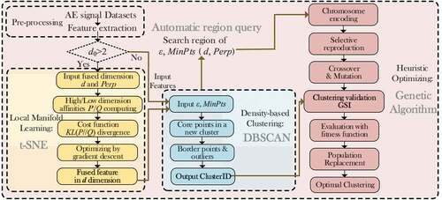
It is obvious that GSI degrades to SI when there is no noise point in clustering. In addition, unlike partition clustering, density-based clustering cannot guarantee that there is more than one cluster in ill-posed parameterization where silhouette is undefined. Based on the proposed GSI, the flowchart for the joint optimization of feature fusion and clustering processes is shown in Figure 3. The proposed method automatically determines the unknown parameters and jointly optimizes feature fusion and clustering by evaluating the proposed validation indices.

Figure 3. The flowchart for automatic and joint optimization of the feature fusion and clustering processes in AE signal analysis.

Clustering Validations of Synthetic and Real-world Benchmark Datasets

In general, clustering techniques perform poorly in extreme distributions with imbalances, irregularities, or anomalies. Thus, to testify the basic clustering performance in different scenarios, the proposed method is compared with five representative clustering techniques, including k-means, agglomerative hierarchical clustering (AHC), fast DBSCAN, density peak clustering (DPC) and OPTICS in ten benchmark validation datasets. Validation datasets 1–5 were two-dimensional benchmark synthetic datasets acquired from different references (Rodriguez and Laio 2014; Wang et al. 2020). Datasets 6–10 were high-dimensional real-world datasets, acquired from the UCI machine learning repository (https://archive.ics.uci.edu/ml/index.php). Detailed information on the datasets is listed in Table 1. Note that symbols “√”and “×” in the table denote that there is or there is no such a property in the corresponding dataset. Datasets 1 and 3 are used to assess the clustering performance in irregular geometry. Datasets 2, 4, and 5 evaluate if the clustering techniques work well under a huge number of objects and their robustness in a mass of anomaly interferences. Datasets 6–10 provide an analysis for dealing with real high-dimensional data. As for the comparison methods, the adopted FDBSCAN seeks the optimal Eps at elbow point where a strong bend is located in the kth-nearest distance graph (k= Minpts). OPTICS is not sensitive to the parameters, but it needs them to initialize. Hence, the initial parameters of OPTICS are provided by FDBSCAN. In contrast, the number of clusters is assumed to obtain the best performance for k-means and AHC. The adopted AHC generates the dendrogram by average linkages, and the maximum iteration for k-means is 2000 in the simulation.

Table 1. Benchmark synthetic datasets and real-world datasets used in the validation

Dataset number	Dataset properties
	Name	Categories	Noise	Instances	Dimensions	Clusters
1	Aggregation	Synthetic (Rodriguez and Laio 2014;Wang et al. 2020)	×	1419	2	7
2	Synthetic4k		√	4000	2	5
3	Two moons		×	1502	2	2
4	T4.8k		√	8000	2	6
5	T5.8k		√	8000	2	6
6	Iris	real-world (UCI)	×	150	4	3
7	Wine		×	178	13	3
8	Seeds		×	210	7	3
9	WBC		×	683	9	2
10	Thyroid		×	215	5	3

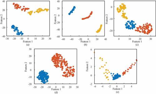
The result visualizations of the proposed method on the above datasets are first shown in Figures 4 and 5. Clusters are marked in different colors. Black points in figures represent identified noise points. Figures 4 and 5 give an intuitive impression that the proposed clustering successfully finds the nature clusters of the data ground-truth. In order to quantify their performance, three external validation metrics of the clustering with different methods are calculated: purity, F₁-measure and adjusted rand index (ARI). Given a priori known classes, purity is an average ratio that the majority class occupies in each cluster as Equation (8)(8) $Purity=\frac{1}{N}\sum _{{\mathbf{C}}_i\in \mathbf{C}}\underset{1\le j\le l}{max}{n}_i^j$(8) , which indicates the probability that individuals of the same class are correctly assigned into the same cluster.

(8) $Purity=\frac{1}{N}\sum _{{\mathbf{C}}_i\in \mathbf{C}}\underset{1\le j\le l}{max}{n}_i^j$(8)

Figure 4. Clustering results of the proposed method on two-dimensional synthetic benchmark datasets: (a) dataset 1, (b) dataset 2, (c) dataset 3, (d) dateset 4 and (e) dataset 5.

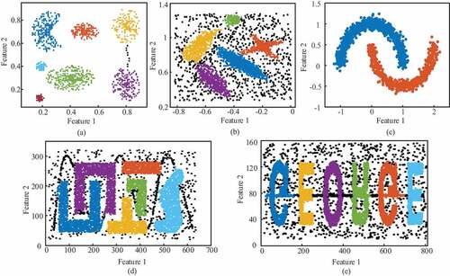
Figure 5. Clustering results of the proposed method on UCI real-world datasets: (a) dataset 6, (b) dataset 7, (c) dataset 8, (d) dataset 9 and (e) dataset 10.

where $n_i^j=\left|{\mathbf{C}}_i\cap {\mathbf{L}}_j\right|$ denotes the total number of the jth class, L_j, contained in cluster C_i and N is the total object number. F₁-measure is rigorously defined as a weighted harmonic average of the precision and recall rate, which provides an assessment considering the distribution of misclassified samples. With l groups of assigned classes, F₁-measure for the entire clustering can be simplified as Equation (9)(9) $F_1=\sum _{j=1}^l\frac{{n{ }^{\mathrm{\prime }}}_j}{N}\underset{{\mathbf{C}}_i\in \mathbf{C}}{max}\left\{\frac{2n_i^j}{n_i+{n{ }^{\mathrm{\prime }}}_j}\right\}$(9) .

(9) $F_1=\sum _{j=1}^l\frac{{n{ }^{\mathrm{\prime }}}_j}{N}\underset{{\mathbf{C}}_i\in \mathbf{C}}{max}\left\{\frac{2n_i^j}{n_i+{n{ }^{\mathrm{\prime }}}_j}\right\}$(9)

where $n{{ }^{\mathrm{\prime }}}_j$ represents the number of objects labeled as jth group and $n_i$ represents the number of objects in ith cluster. The F₁-measure is a useful indication to display the degree of uneven distribution. ARI is a metric that considers the number of object-pairs upon both the agreement and disagreement between the two (clustering) partitions (Vinh, Bailey, and Epps 2010):

(10) $ARI\left(\mathbf{C},\mathbf{L}\right)=\frac{2\left(N_{00}{N}_{11}-N_{01}{N}_{10}\right)}{\left(N_{00}+N_{01}\right)\left(N_{01}+N_{11}\right)+\left(N_{00}+N_{10}\right)\left(N_{10}+N_{11}\right)}$(10)

where N₁₁ is the number of object-pairs belonging to the same clusters in both C and L, N₀₀ is the number of pairs belonging to different clusters in both partitions, N₁₀ is pair number belonging to same cluster in C but different clusters in L, and N₀₁ is the number of converse cases against N₁₀.

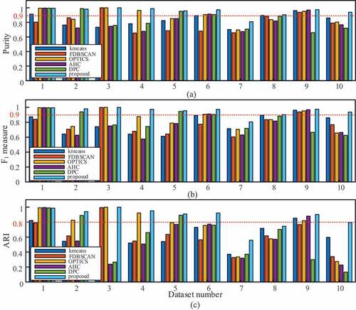
Purity can be regarded as the overall accuracy, and F₁-measure gives a better indication of the imbalance in the misidentified samples. In contrast, the adjusted rand index has a better penalty effect on cluster splitting/merging and drops remarkably when the cluster numbers differ in two partitions. Note that the clustering with metric values all larger than the thresholds of purity (>0.9), F₁-measure (>0.9) and ARI (>0.8) indicates a better result. The results of all the methods on the above datasets (No.1–10) are assessed with the purity, F₁-measure and ARI of different clustering. The validating performance of the comparison methods is shown in Figure 6. DPC, AHC and k-means succeeded in dataset 1 (ARI>0.8) but failed to extract the clusters in irregular dataset 3 (ARI<0.3) even though the latter dataset is much simpler. Centroid-based clustering mechanisms cannot work well when the clusters penetrate into each other because the centroid-distance contradicts the majority of the cluster objects and violates the Guassian-distributed assumption in this context. Regarding the robustness for mass data and amonalies, most clustering techniques lack robustness when dealing with anomalies. Only the density-based techniques (except FDBSCAN) can separate true clusters from outliers in datasets 2, 4, and 5. The performance of FDBSCAN is unstable (F₁-measure<0.7, ARI<0.65) in this case considering that the elbow points of the k-dist-graph tend to be critical values of ruling out outliers instead of the true optimum for separability. The proposed method provides the highest average ARI (0.784 ± 0.146) from datasets 6 to 10. When dealing with high-dimensional data, t-SNE plays an important role of a feature refiner for the proposed method, which evolves capturinge the discriminative structure and eventually offering the representation of clustering-friendly features. The proposed method overwhelmingly outperforms the others in terms of the stability of all validations, which implies that it gives a reliable indication for natural clusters in arbitrary distribution and heavy interference of amonalies. OPTICS obtained the second highest ARI in 2D datasets, which is slightly lower than the proposed method. K-means provides the second highest ARI (0.653 ± 0.181) in real-world datasets, for it is insenstive to data dimension.

Figure 6. (a) Purity, (b) F₁-measure and (c) ARIs of the comparing methods in the validating datasets (No. 1–10 in Table 1).

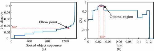
In terms of region query efficiency, the proposed method is compared with the FDBSCAN. Assuming that Minpts in dataset 1 equals 10, region query curves of both methods are shown in Figure 7. In Figure 7a, the elbow point in kth-distance graph shows a sharp rise that separates a mass of noise from the dataset, but the solution Eps* is unreliable in discovering the latent cluster structure. Comparatively, the feasible solution of Eps in Figure 7b is divided into several regions. When Eps is too small, a true cluster is misidentified as subclusters, and the proposed penalty will lessen GSI to mitigate. In contrast, when Eps far exceeds the expected threshold, some features are overlooked and clusters are merged together. As long as the partition is identical, the evaluation performance is stable within the region. The above analysis shows that the generalized silhouette index gives a robust clustering quality with suiteable solutions Eps* and all the natural clusters are successfully identified.

Figure 7. Region query in dataset 1 with (a) k-dist graph (Minpts = 10) and (b) GSI.

Besides, the theoretical computational complexity of the aforementioned methods are listed in Table 2, where K, I and n denote the number of predefined clusters, iterations and objects, respectively. P denotes the number of individuals in the population for genetic optimization. The complexity of the dimension reduction step (Linderman et al. 2019), density-based clustering step and genetic operations is O(nlogn), O(nlogn), and O(P²), respectively. Therefore, the overall computational complexity of the proposed method is O(P²nlogn). Since the population size is normally predefined and far less than the object number in such problems, whose effect on the increase of computational cost with increasing objects is equivalent to a constant for the proposed method. Consequently, the computational efficiency of the proposed method is higher in large databases (n> P²) than the improved density-based clustering, although its computational cost is multiple times that of FDBSCAN.

Table 2. Theoretical computational complexity of the mentioned clustering methods

Algorithms	k-means	AHC	FDBSCAN	OPTICS	DPC	Proposed method
Complexity	O(KIn)	O(n^3)	O(nlogn)	O(n^2logn)	O(n^2)	O(P^2nlogn)

Experiment and Datasets

The proposed method is further verified with actual AE signals obtained from the tensile test, which records AE signals from the entire fracture process and carries essential information for rail steel health analysis. A schematic diagram of the test system is illustrated in Figure 8a,b. It consists of three main parts: a test specimen, a tensile testing machine and an AE data acquisition system.

Figure 8. (a) Schematic diagram of the tensile test system, (b) a closeup of the tensile testing machine and (c) a photo of the specimen and U75V rail steel.

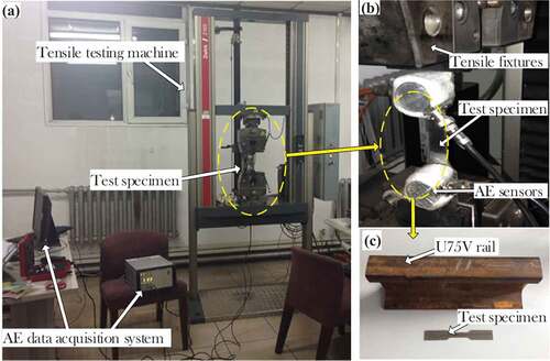
The test specimen was made from U75V rail steel, as shown in Figure 8c. The fracture process of test specimen was performed using a tensile testing machine (Model: Zwick Z100). In this experiment, small-scale U75V specimens are tested under pure tensile loading to analyze the fracture process of rail steel. During the test, AE data is acquired by an AE data acquisition system (Model: Vallen AMSY-6 ASIP-2/A) with a sampling rate of 5 MHz. AE sensors (Model: Vallen VS900-RIC) are attached on the specimen. Then, the tension is applied to the specimen until it fractures. A tensimeter is used to measure the tensile stress, and burst-type AE signals are acquired synchronously.

The fracture of the specimen is a gradual process, and AE signals are roughly divided by the stress-strain curve into three stages: initial stage, crack propagation and brittle fracture (Zhang et al.2015a). Signals of these stages are obtained in time order, labeled according to their collection time. Four tensile tests are carried out, and the obtained datasets are used in the clustering analysis. Additionally, mechanical noise signals acquired with the same acquisition apparatus under the actual operating railway are also used here as noise interference in the random noise test. Noise signals are normally generated by wheel-rail interactions, and a detailed description of the railway noise has been provided previously (Wang et al. 2019).

Results and Discussions

In this section, the proposed method is applied to an actual AE dataset obtained from the tensile test and noise from a real operating railway to validate its practicability. How the proposed method outperforms the other algorithms in capturing the natural clusters of AE signals from different rail health stages is also illustrated. The failure mechanisms behind these clusters are analyzed as a supplement.

Feature Extraction of AE Signals

In rail health analysis, the feature extraction process determines the clustering performance to a large extent. To extract the frequency features of transient AE signals, wavelet analysis is validated to outperform the other decomposition methods. In particular, wavelet packet transformation (WPT) gets superior performance with high resolution in a high-frequency band, and it is applied in this research. Daubechies 11 (db11) is chosen as the mother wavelet according to a previous research (Hao et al. 2018). AE signals here are decomposed by a three-layer wavelet packet. Assuming that $d_{j,k}\left(t\right)$ are the wavelet packet coefficients for all k translations at scale j, the average energy ratios of coefficients p_i are used as frequency features,, where $p_i=E_i/{\sum }_{j=1}^n{E}_j$ and $E_j=\frac{1}{N_j}\sum _{k=1}^{N_j}{\left[d_{j,k}\left(t\right)\right]}^2$. Such a wavelet parameter gives proportion information of the spectrum components instead of peak frequency and centroid frequency. Furthermore, the integrated wavelet energy distribution is quantitatively described as another feature measured by wavelet entropy, $E_{entropy}=-\sum _{i=1}^n{p}_i{log}_2{p}_i$ (Zhang et al. 2015b).

Since the common acoustic emission frequency band is predominantly distributed below 1 MHz, only the first five scales (1.56 MHz) of the energy coefficients are utilized in the analysis. All adopted discriminative features for AE signals are summarized in Table 3, including dimensionless features and those in time–frequency domain. The dimensions of all features (d₀) are 15, and all the features are standardized to be within [−1, 1].

Table 3. Discriminative features for AE signal clustering

Feature No.	Feature type	Feature name
1–6	Frequency domain	Wavelet packet coefficient energy ratio; Wavelet entropy
7–9	Time domain	Peak value; Absolute mean; Root mean square
10–15	Dimensionless	Skewness; Kurtosis; Crest factor; Waveform factor; Pulse factor; Clearance factor

Inherent Principle in Region Query of t-SNE

Typically, raw features are ordinary high-dimensional data containing the redundancy and irrelevance. Thus, feature fusion is of significant importance in mapping the raw features into the latent representation. T-SNE has been broadly acknowledged as a dimensionality reduction and visualization method. There have been some preliminary studies about tuning perplexity in t-SNE with various validation indices, among which silhouette-based indices have been revealed commonly effective in real-world data (Devassy, George, and Nussbaum 2020). Hopefully, they imply that GSI has the potential to harmonize both automatic region queries for clustering and t-SNE.

To obtain optimal traits for AE data, the t-SNE feature quality is evaluated quantitatively with GSI. Together with perplexity, the fused feature dimension is considered. An intuitive illustration, the grid-search graph for the t-SNE parameter tuning based on test 1 is shown in Figure 9. Each point in Figure 9 represents a maximum in clustering validation based on GSI with certain Perp and feature dimension. Notably, as the fused dimension increases, the features become less discriminative with a descending tendency for the optimal GSI. GSIs of different dimensions vary in a range from 0.6282 to 0.4954. The most discriminative features in this test are obtained in t-SNE 2-D mapping. On the other hand, when a fused dimension is fixed, a potential unimodal GSI distribution with single peak for Perp could be viewed and interpreted: if Perp is too small, t-SNE is dominated with the closest neighbors and the distribution is split into wrong subclusters. While Perp is too large, global silhouette dominates and all the points are compact as an indivisible integral. Additionally, as Figure 9 shows, the optimal size of perplexity is highly related to the fused dimension and the total number of samples. The optimal perplexity (with maximum GSI) gradually shifts toward smaller values (without abrupt jumps or drops) between adjacent dimensions when the fused dimension increases. However, the heuristic search of GA is necessary to eliminate of the sensitivity effect of t-SNE parameters to provide acceptable clustering-friendly features.

Figure 9. Optimization of t-SNE based on GSI for test 1.

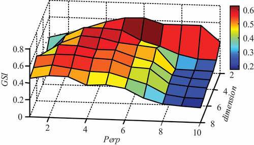
In essence, t-SNE plays the role of a feature refiner that evolves to capture the discriminative structure and eventually offers the optimal representation of clustering-friendly features. In this case, 2-D features with Perp = 30 are the most discriminative among all representations for test 1 and will be provided to the comparative methods as fused features to eliminate feature influence among different clustering techniques.

Related Fracture Mechanism and Efficiency of Clustering

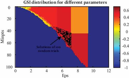
In order to understand the efficiency and stability of hyperspace region query, a fine-grid subspace map (interval of Eps is 0.01) shows the GSI distribution for different parameters in test 1, as shown in Figure 10. The feasible region with the highest objective value is composed of appropriate combinations of ε and Minpts. A smaller range of ε indicates DBSCAN is normally more sensitive to ε. Also, 100 random repeated trials of the proposed method were implemented, and the solutions are also scattered as black points in the map. Theoretically, DBSCAN is so robust that the resultant partition remains identical within a certain solution area, which could be portrayed as a step-shape. A restrictive relation between parameters can also be seen in Figure 10, which validates a situation without available gradients as mentioned. However, the stability of the genetic searching can be clearly seen in the solutions distributions of 100 random repeated trials in Figure 10. All solutions are uniformly distributed within the area with the highest GSI (0.6282) representing the optimal partition results in this scenario.

Figure 10. GSI distribution map for different parameters in clustering.

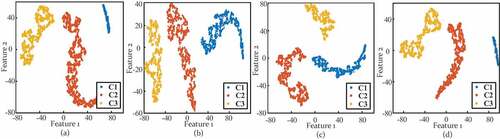
Eventually, clustering visualization of all the tensile AE datasets is presented in Figure 11. Through the analysis, all the AE datasets are distinguished into three groups in 2-D feature space. The visualization shows that points are close to the allocated cluster and distant from the alternative clusters. Moreover, the mechanisms behind the clusters could be interpreted in accordance with the time/strain records of specimen fractures: the majority of each identified cluster in these figures is assigned to a certain damage mechanism and correlates with different stages in the temporal evolution of the AE data. Most objects in C₁ belong to elastic dislocations with yielding sources. The specimen is rather inactive, with fewer AE events, collected from the healthy stage. On the other hand, C₂ represents the crack propagation stage, ascribed to light damage such as micro-cracking and propagation of cracks with high-frequency components up to 800 kHz. Cluster C₃ means the heavy damage stage when necking and macro cracks generated, which can be visualized at the surface of the specimen.

Figure 11. Visualization of clusters from (a) test 1, (b) test 2, (c) test 3 and (d) test 4 datasets in 2D features fused by t-SNE.

Clustering Validations and Robustness Discussions

To validate the clustering performance systematically, external validation indices are applied to quantify the number of correctly identified objects. Thereby, all tensile datasets were testified on original features and t-SNE fused features, with k-means, AHC, fast DBSCAN, the proposed method and another density-based clustering technique, OPTICS. External validation of cluster purity and F₁-measure of different algorithms are displayed in Figure 12.

Figure 12. (a) Purities and (b) F1-measure of tensile tests in accordance with stage labels.

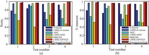
As Figure 12 illustrates, the proposed method exhibits a much higher accuracy on average (0.974 ± 0.012) than k-means (0.869 ± 0.073) and AHC (0.960 ± 0.014). The proposed method significantly improves the density-based clustering performance by solving the optimal region query and eliminating the curse of dimensionality, while OPTICS is insensitive to the ε and obtains the second highest accuracy (0.969 ± 0.015) with fused features in tensile data. The clustering accuracy with t-SNE fused features increases 0.434 for density-based clustering on average, compared with the accuracy with raw AE features and 0.25 for the hierarchical model. Furthermore, the robustness and applicability of the proposed method is compared with those of AHC and OPTICS in a random test with mechanical noise. In this test, 100 samples of each stage are stochastically chosen from all the tensile datasets in section 4.3, and these samples are mixed with different proportions of the actual railway operating noise. The total number of randomly selected noise samples ranges from 100 to 1000, which simulates the highly imbalanced data structure acquired in an actual operating railway. The algorithms are assessed by external validation indices under mechanical noise, and the visualized clustering results of proposed method are shown in Figure 13a,b (noise cluster labeled as ‘N_n’).

Figure 13. Clustering results of proposed method in random noise tests with a number of (a) 100, (b) 200 railway noise samples and (c) purities and F₁-measures for the proposed method, OPTICS and AHC under variant noise interference.

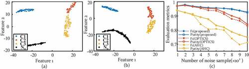
As seen in Figure 13c, F₁-measure and purity for the proposed method are in good agreement (between 0.928 and 0.986), which remain stable and show robustness in the noisy/uneven dataset structure when the proportion of railway noise increases. The majority of the wrongly categorized samples are signals from stage 2, stage 3 and noise, misclassified into each other. Evaluations of comparative methods diminish rapidly (0.159 for AHC and 0.108 for OPTICS) when the noise sample numbers are more than 300 and 600, respectively. The F₁-measure virtually falls more sharply than purity when the incorrect samples are unevenly distributed (systematic bias due to imbalance). In AHC assessments, F₁-measure is much lower than purity, implying that the misclassified samples are unevenly distributed and mostly identified as the dominant cluster. This deficiency leads to a systematic bias in the resultant partition. Degradation in OPTICS ascribed to the instability of the automatic cluster extraction process, which failed to provide a consistent extracting criterion under variant conditions when noise samples is larger than 600. From the above aspects, it is apparent that the proposed method accurately identifies the nature clusters in all tensile tests and improves the stability and robustness of clustering technique under railway operating noise. The contributions of the proposed method to density-based clustering are summarized as follows: (1) a genetic fine-tuning technique is first introduced into DBSCAN to solve its extreme sensitivity to two priory parameters; (2) aiming for a promotion of the robustness to anomalies and outliers, a generalized silhouette index (GSI) was proposed to assist the optimization of clustering parameters; (3) to overcome the curse of dimensionality and enhance its efficiency in high-dimensional data, t-SNE is also combined in the joint optimization to automatically obtain the clustering-firendly latent features. The innovation and insights of this paper have the potential to predict the patterns of other real-world engineering datasets and might help to provide a guidance in similar tasks of discovering intrinsic engineering data groups. However, it is undeniable that even the proposed clustering technique highly depends on the implicit assumption of density-connectivity inside a cluster and the ensemble clustering technique might be a good choice for robust consensus clustering without assumption restraints in the future extension of this study (Huang et al. 2021, 2020).

Conclusion

In this study, a novel genetic density-based clustering integrated with t-SNE is proposed and its utility is investigated to discover relevant rail health stages from AE signals. An automated genetic strategy is employed for region queries, and a generalized silhouette index is advanced, which can evaluate the clustering performance and handle noise properly. Note that the proposed method does not require any prior information and simplify the application of clustering to a large extent. The proposed algorithm is initially validated in five benchmark 2-D synthetic datasets and five real-world datasets, which perform superiorly in irregular shapes and noisy datasets. Subsequently, it is applied in clustering AE data of tensile tests and enhances the distinguishability of the raw AE features. The reliability of its genetic optimization is also tested and the mechanisms related to each cluster were thereafter elucidated. Eventually, the proposed method was validated through random tests with an increasing proportion of actual railway operating noise. The results show that the proposed method outperforms the comparative methods in categorizing the AE features and its high robustness is revealed under a large proportion of mechanical noise in rail health analysis.

Disclosure statement

No potential conflict of interest was reported by the author(s).

Additional information

Funding

This research was supported by the National Natural Science Foundation of China [No. 62033004 and No. 61771161], the China Railway Harbin Group Co., Ltd, the National Key R&D Program of China [No. 2019YFC0117400] and the foundation of China Scholarship Council [No. 201906120066].

References

- Alahakoon, S., Y. Sun, M. Spiryagin, and C. Cole. 2018. Rail flaw detection technologies for safer. Reliable Transportation: A Review, Journal of Dynamic Systems, Measurement and Control 140 (2):298–322.
- Amorim, R. C. D., and C. Hennig. 2015. Recovering the number of clusters in data sets with noise features using feature rescaling factors. Information Science 324:126–45. doi:10.1016/j.ins.2015.06.039.
- Angelopoulos, N., and M. P. Papaelias. 2018. Automated analysis of acoustic emission signals based on the ISODATA algorithm. Insight-Non-Destructive Testing and Condition Monitoring 60 (3):130–38. doi:10.1784/insi.2018.60.3.130.
- Behnia, A., H. K. Chai, M. GhasemiGol, A. Sepehrinezhad, A. A. Mousa. 2019. Advanced damage detection technique by integration of unsupervised clustering into acoustic emission. Engineering Fracture Mechanics 210:212–27. doi:10.1016/j.engfracmech.2018.07.005.
- Borah, B., and D. K. Bhattacharyya. 2004. An improved sampling-based DBSCAN for large spatial databases. Proceedings of International Conference on Intelligent Sensing and Information Processing (ICISIP), Chennai, India, pp. 92–96.
- Devassy, B. M., S. George, and P. Nussbaum. 2020. Unsupervised clustering of hyperspectral paper data using t-SNE. Journal of Imaging 6 (29):1–12. doi:10.3390/jimaging6010001.
- Ester, M., H. P. Kriegel, J. Sander, and X. Xu. 1996. A density-based algorithm for discovering clusters in large spatial data bases with noise. Proceedings of the 2nd International Conference on Knowledge Discovery and Data Mining, Portland, USA, pp. 226–31.
- Fukui, K. I., K. Sato, J. Mizusaki, and Numao, M. 2010. Kullback-Leibler divergence based kernel SOM for visualization of damage process on fuel cells. Proceedings of 22nd IEEE International Conference on Tools with Artificial Intelligence, Arras, France.
- Galán, S. F. 2019. Comparative evaluation of region query strategies for DBSCAN clustering. Information Science 502:76–90. doi:10.1016/j.ins.2019.06.036.
- Gong, Y., S. Lin, F. He, Y. He, and J. Song. 2021. Damage identification of prefabricated reinforced concrete box culvert based on improved Fuzzy clustering algorithm and acoustic emission parameters. Advances in Materials Science and Engineering 2021:6660915. doi:10.1155/2021/6660915.
- Hao, Q., X. Zhang, K. Wang, Y. Shen, Y. Wang. 2018. A signal-adapted wavelet design method for acoustic emission signals of rail cracks. Applied Acoustics 139:251–58. doi:10.1016/j.apacoust.2018.04.038.
- Huang, D., C. D. Wang, H. Peng, J. Lai, C.-K. Kwoh. 2021. Enhanced ensemble clustering via fast propagation of cluster-wise similarities. IEEE Transcations on Systems, Man, and Cybernetics: Systems. 51(1):508–20. doi:10.1109/TSMC.2018.2876202.
- Huang, D., C. D. Wang, J. Wu, J.-H. Lai, C.-K. Kwoh. 2020. Ultra-scalable spectral clustering and ensemble clustering. IEEE Transcations on Knowledge Discovery and Data Mining. 32(6):1212–26. doi:10.1109/TKDE.2019.2903410.
- Jiang, H., J. Li, S. Yi, X. Wang, X. Hu. 2011. A new hybrid method based on partitioning-based DBSCAN and ant clustering. Expert Systems with Applications. 38(8):9373–81. doi:10.1016/j.eswa.2011.01.135.
- Linderman, G. C., M. Rachh, J. G. Hoskins, S. Steinerberger, Y. Kluger. 2019. Fast interpolation-based t-SNE for improved visualization of single-cell RNA-seq data. Nature Methods. 16(3):243–45. doi:10.1038/s41592-018-0308-4.
- Liu, B. 2006. A fast density-based clustering algorithm for large databases. Proceedings of 5th International Conference on Machine learning and Cybernetics, Dalian, China.
- Liu, J., Y. Hu, B. Wu, and Y. Wang. 2018. An improved approach for FDM process with acoustic emission. Journal of Manufacturing Processes 35:570–79. doi:10.1016/j.jmapro.2018.08.038.
- Liu, Y., Z. Li, H. Xiong, X. Gao, J. Wu, S. Wu. 2013. Understanding and enhancement of internal clustering validation measures. IEEE Transactions on Cybernetics. 43(3):982–94. doi:10.1109/TSMCB.2012.2220543.
- Maaten, L. V. D., and G. Hinton. 2008. Visualizing data using t-SNE. Journal of Machine Learning Research 9 (85):2579–605.
- Olofsson, U., and R. Nilsson. 2002. Surface cracks and wear of rail: A full-scale test on a commuter train track. Proceedings of the Institution of Mechanical Engineers Part F Journal of Rail & Rapid Transit 216 (4):249–64. doi:10.1243/095440902321029208.
- Parmar, M., D. Wang, X. Zhang, A. Tan, C. Miao, J. Jiang, Y. Zhou. 2019b. REDPC: A residual error-based density peak clustering algorithm. Neurocomputing 348:82–96. doi:10.1016/j.neucom.2018.06.087.
- Parmar, M., W. Pang, D. Hao, J. Jiang, W. Liupu, L. Wang, Y. Zhou. 2019a. FREDPC: A feasible residual error-based density peak clustering algorithm with the fragment merging strategy. IEEE Access 7:89789–804. doi:10.1109/ACCESS.2019.2926579.
- Rodriguez, A., and A. Laio. 2014. Clustering by fast search and find of density peaks. Science 344 (6191):1492–96. doi:10.1126/science.1242072.
- Rousseeuw, P. J. 1987. Silhouettes: A graphical aid to the interpretation and validation of cluster analysis. Journal of Computational and Applied Mathematics 20:53–65. doi:10.1016/0377-0427(87)90125-7.
- Saeedifar, M., M. A. Najafabadi, D. Zarouchas, H. H. Toudeshky, M. Jalalvand. 2018. Clustering of interlaminar and intralaminar damages in laminated composites under indentation loading using Acoustic Emission. Composites Part B: Engineering 114:206–19. doi:10.1016/j.compositesb.2018.02.028.
- Schneider, J., and M. Vlachos. 2017. Scalable density-based clustering with quality guarantees using random projections. Data Mining and Knowledge Discovery 31 (4):972–1005. doi:10.1007/s10618-017-0498-x.
- Sibil, A., N. Godin, M. R’Mili, E. Maillet, G. Fantozzi. 2012. Optimization of acoustic emission data clustering by a genetic algorithm method. Journal of Nondestructive Evaluation. 31(2):169–80. doi:10.1007/s10921-012-0132-1.
- Synodinos, A. 2016. Identification of railway track components and defects by analysis of wheel-rail interaction noise. Proceedings of 23rd International Congress on Sound and Vibration, Athens, Greece.
- Valdes, J. J., C. Cheung, and A. L. Rubio. 2017. Extreme learning machines to approximate low dimensional spaces for helicopter load signal and fatigue life estimation. Proceedings of International Joint Conference on Neural Networks, Portland, USA.
- Vinh, N. X., J. C. Bailey, and J. Epps. 2010. Information theoretic measures for clusterings comparison: Variants, properties, normalization and correction for chance. Journal of Machine Learning Research 11:2837–54.
- Wang, K., X. Zhang, Q. Hao, Y. Wang, Y. Shen. 2019. Application of improved least-square generative adversarial networks for rail crack detection by AE technique. Neurocomputing 332:236–48. doi:10.1016/j.neucom.2018.12.057.
- Wang, Y., D. Wang, W. Pang, C. Miao, A.-H. Tan, Y. Zhou. 2020. A systematic density-based clustering method using anchor points. Neurocomputing 400:352–70. doi:10.1016/j.neucom.2020.02.119.
- Yang, L., H. S. Kang, Y. C. Zhou. 2015. Frequency as a key parameter in discriminating the failure types of thermal barrier coatings cluster analysis of acoustic emission signals. Surface and Coating Technology. 264:97–104.
- Zhang, X., K. Wang, Y. Wang, Y. Shen, H. Hu. 2020. Rail crack detection using acoustic emission technique by joint optimization noise clustering and time window feature detection. Applied Acoustics 160:1–13. doi:10.1016/j.apacoust.2019.107141.
- Zhang, X., N. Feng, Y. Wang, and Y. Shen. 2015b. Acoustic emission detection of rail defect based on wavelet transform and Shannon entropy. Journal of Sound and Vibration 339:419–32. doi:10.1016/j.jsv.2014.11.021.
- Zhang, X., N. Feng, and Z. Zou, et al. 2015a. An investigation on rail health monitoring using acoustic emission technique by tensile test. Proceedings of Instrumentation and Measurement Technology Conference (I2MTC), Pisa, Italy.