A Novel Machine Learning Based Framework for Detection of Autism Spectrum Disorder (ASD)

ABSTRACT

Autism Spectrum Disorder (ASD) is linked with abridged ability in social behavior. Scientists working in the broader domain of cognitive sciences have done a lot of research to discover the root cause of ASD, but its biomarkers are still unknown. Some studies from the domain of neuroscience have highlighted the fact that corpus callosum and intracranial brain volume hold significant information for the detection of ASD. Taking inspiration from such findings, in this article, we have proposed a machine learning based framework for automatic detection of ASD using features extracted from corpus callosum and intracranial brain volume. Our proposed framework has not only achieved good recognition accuracy but has also reduced the complexity of training machine learning model by selecting features that are most significant in terms of discriminative capabilities for classification of ASD. Second, for benchmarking and to verify potential of deep learning on analyzing neuroimaging data, in this article, we have presented results achieved by using the transfer learning approach. For this purpose, we have used the pre-trained VGG16 model for the classification of ASD.

Introduction

The emerging field of computer vision and artificial intelligence has dominated research and industry in various domains and is now aiming to outstrip human intellect (Sebe et al. 2005). With computer vision and machine learning techniques, unceasing advancement has been made in different areas like imaging (Kak and Slaney 1988), biometric systems (Munir and Khan 2019), computational biology (Zhang 2002), video processing (Van Den Branden Lambrecht 2013), affect analysis (Khan et al. 2019b; Khan, et al., 2013a, Khan, et al., 2013b, Khan, 2013c), medical diagnostics (Akram et al. 2013), cybersecurity (Nazir and Khan 2021), image synthesis (Crenn et al. 2020), electronic health records (Shah and Khan 2020) and much more. However, despite all the advances, neuroscience is one of the areas in which machine learning is minimally applied due to the complex nature of data. This article proposes a framework for automatic identification of Autism Spectrum Disorder (ASD) (Jaliaawala and Khan 2019) by applying the machine learning algorithm on the neuroimaging dataset known as ABIDE (Autism Brain Imaging Data Exchange) (Di Martino et al. 2014).

Autism Spectrum Disorder (ASD) is a neurodevelopmental disorder that is perceived by a lack of social interaction and emotional intelligence, repetitive, abhorrent, stigmatized and fixated behavior (Choi 2017; Jaliaawala and Khan 2019). This syndrome is not a rare condition, but a spectrum with numerous disabilities. ICD-10 WHO (World Health Organization 1993) (Organization 1993) and DSM-IV APA (American Psychiatric Association) (Castillo et al. 2007) outlined criteria for defining ASD in terms of social and behavioral characteristics. According to their nomenclature, an individual facing ASD has an abnormal trend associated with social interaction, lack of verbal and non-verbal communication skills and a limited range of interests in specific tasks and activities (Jaliaawala and Khan 2019). Based on these behavioral lineaments, ASD is further divided into groups, which are as follows:

1. High Functioning Autism (HFA) (Baron-Cohen et al. 2001): HFA is a term applied to people with autistic disorder, who are deemed to be cognitively “higher functioning” (with an IQ of 70 or greater) than other people with autism.

2. Asperger Syndrome (AS) (Klin, Volkmar, and Sparrow 2000): individuals facing AS have qualitative impairment in social interaction and show restricted repetitive and stereotyped patterns of behavior, interests, and activities. Usually, such individuals have no clinically significant general delay in language or cognitive development. Generally, individuals facing AS have higher IQ levels but lack in facial actions and social communication skills.

3. Attention Deficit Hyperactivity Disorder (ADHD) (Barkley and Murphy 1998): individuals with ADHD show impairment in paying attention (inattention). They have overactive behavior (hyperactivity) and sometimes impulsive behavior (acting without thinking).

4. Psychiatric symptoms (Simonoff et al. 2008), such as anxiety and depression.

Recent population-based statistics have shown that autism is the fastest-growing neurodevelopmental disability in the United States and the UK (Rice 2009). More than 1% of the children and adults are diagnosed with autism, and costs of $2.4 million and $2.2 million are used for treatment in the United States and the United Kingdom, respectively, as reported by the Center of Disease Control and Prevention (CDC), USA (Buescher et al. 2014; Rice 2009). It is also known that delay in detection of ASD is associated with increase in cost for supporting individual with ASD (Horlin et al. 2014). Thus, it is utmost important for research community to propose novel solutions for early detection of ASD and our proposed framework can be used for early detection of ASD.

Until now, biomarkers of ASD are unknown (Del Valle Rubido et al. 2018; Jaliaawala and Khan 2019). Physicians and clinicians are practicing standardized/conventional methods for ASD analysis and diagnosis. Intellectual properties and behavioral characteristics are accessed for the diagnosis of ASD; however, synaptic affiliations of ASD are still unknown and presents a challenging task for cognitive neuroscience and psychological researchers (Kushki et al. 2013). A recent hypothesis in neurology demonstrates that an abnormal trend is associated with different neural regions of the brain among individuals facing ASD (Bourgeron 2009). This variational trend is due to irregularities in neural pattern, disassociation and anti-correlation of cognitive function between different regions that affect the global brain network (Schipul, Keller, and Just 2011).

Magnetic Imaging Resonance (MRI), a noninvasive technique, has been widely used to study the brain regional network(s). Thus, MRI data can be used to reveal subtle variations in neural patterns/network, which can help in identifying biomarkers for ASD. An example of MRI scan in different cross-sectional view is shown in Figure 1. MRI scans are further divided into structural MRI (s-MRI) and functional MRI (f-MRI) depending on the type of scanning technique used (Bullmore and Sporns 2009). Structural MRI (s-MRI) scans are used to examine anatomy and neurology of the brain. s-MRI scans are also employed to measure the volume of brain, i.e. regional gray matter (GM), white matter (WM) and cerebrospinal fluid (CSF) (Giedd 2004), and volume of its sub-regions and to identify localized lesions (Budman, Hoyt, and Friedman 1992). Functional MRI (f-MRI) scans are used to visualize the activated brain regions associated with brain function. f-MRI computes synchronized neural activity through the detection of blood flow variation across different cognitive regions. By using MRI scans, numerous researchers have reported that distinctive brain regions are associated with ASD (Huettel, Song, and McCarthy et al. Huettel, et al., 2004).

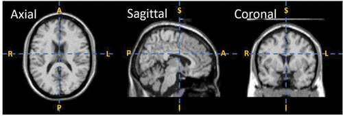
Figure 1. MRI scan in different cross-sectional views, where A, P, S, I, R, and L in the figure represent anterior, posterior, superior, inferior, right, left, respectively. The axial/horizontal view divides the MRI scan into head and tail/superior and inferior portions, sagittal view breaks the scan into left and right and coronal/vertical view divides the MRI scan into anterior and posterior portions (Schnitzlein and Murtagh 1985).

In 2012, the Autism Brain Imaging Data Exchange (ABIDE) provided scientific community with an “open source” repository to study ASD from brain imaging data i.e. MRI data (Di Martino et al. 2014). The ABIDE dataset consists of 1112 participants (autism and healthy control) with rs-fMRI (resting state functional magnetic resonance imaging) data. rs-fMRI is a type of f-MRI data captured in resting or task-negative state (Plitt, Barnes, and Martin 2015; Smith et al. 2009). ABIDE also provides anatomical scans and phenotypical¹ data (Di Martino et al. 2014). All the details (data collection and preprocessing) related to ABIDE dataset are presented in Section 3.

In this study, we have proposed a machine learning based framework for automatic detection of ASD using T1-weighted MRI scans from from ABIDE dataset. T1-weighted MRI data is used as it is reported that results from T1-weighted MRI data are highly reproducible (McGuire et al. 2017). Initially, for automatic detection of ASD, we have utilized different conventional machine learning methods (refer Section 4.1.2 for details of machine learning algorithms used in this study). Conventional machine learning methods refer to methods other than recently popularized deep learning approach. We further improved results achieved by conventional machine learning methods by calculating importance/weights of different features for the given task (Section 4.1.1 presents feature selection methodology employed in this study). Features are measurable attribute of the data (Bishop 2006). Feature selection methods find weights/importance of different features by calculating their discriminative ability, thus improving the prediction performance, computational time and generalization capability of the machine learning algorithm (Chandrashekar and Sahin 2014). Results obtained by applying feature selection methods and conventional machine learning methods are discussed in Section 4.1.3. Finally, to verify the potential of deep learning (LeCun, Bengio, and Hinton 2015) on analyzing neuroimaging data, we have done experiment with the state-of-the-art deep learning architecture, i.e. VGG16 (Simonyan and Zisserman 2014). We have used the transfer learning approach (Khan, et al., 2019a) to use already trained VGG16 model for detection of ASD. Results obtained using transfer learning approach are presented in Section 4.2. Section 4.2 will help readers to understand benefits and bottlenecks of using the deep learning/CNN approach for analyzing neuroimaging data, which is difficult to record in a large enough quantity for deep learning. Survey of the related literature is presented in the next section, i.e. Section 2.

In summary, our contributions in this study are as follows:

1. We showed potential of using machine learning algorithms applied to brain anatomical scans for automatic detection of ASD.

2. This study demonstrated that feature selection/weighting methods helps to achieve better recognition accuracy for detection of ASD.

3. We also provided automatic ASD detection results using deep learning (LeCun, Bengio, and Hinton 2015)/Convolutional Neural Networks (CNN) via the transfer learning approach. This will help readers to understand benefits and bottlenecks of using the deep learning/CNN approach for analyzing neuroimaging data, which is difficult to record in large enough quantity for deep learning.

4. We also highlighted future directions to improve the performance of such frameworks for automatic detection of ASD. Thus, such frameworks could perform well not only for published databases but also for real world applications and help clinicians in early detection of ASD.

State of the Art

In this section, various methods that have been explored for the classification of neurodevelopmental disorders are discussed but focus remains on the detection of ASD. Fusion of artificial intelligence techniques (machine learning and deep learning) with brain imaging data has allowed to study the representation of semantic categories (Haxby et al. 2001), meaning of noun (Buchweitz et al. 2012), learning (Bauer and Just 2015) and emotions (Kassam et al. 2013). But, general use of machine learning algorithms to detect psychological and neurodevelopmental ailments, i.e. schizophrenia (Bellak 1994), autism (Just et al. 2014) and anxiety/depression (Craddock et al. 2009), remains restricted due to the complex nature of problem.

Craddock et al. (Cameron Craddock and Holtzheimer 2009) used the multi-voxel pattern analysis technique for the detection of Major Depressive Disorder (MDD) (Greicius et al. 2007). They have shown results on MRI data gathered from forty subjects, i.e. twenty healthy controls and twenty individuals with MDD. Their proposed framework achieved an accuracy of 95%. Just et al. (Just et al. 2014) presented the Gaussian Naïve Bayes (GNB) classifiers based approach to identify ASD and control participants using fMRI data. They achieved accuracy of 97% while detecting autism from a population of 34 individuals (17 control and 17 autistic individuals).

One of the promising studies done by Sabuncu et al. (Sabuncu et al. 2015) used the Multivariate Pattern Analysis (MVPA) algorithm and structural MRI (s-MRI) data to predict chain of neurodevelopmental disorders i.e. Alzheimer’s, Autism, and Schizophrenia. Sabuncu et al. analyzed structural neuroimaging data from six publicly available websites (https://www.nmr.mgh.harvard.edu/lab/mripredict), with 2800 subjects. The MVPA algorithm constituted with three classes of classifiers that includes a Support Vector Machine (SVM) (Vapnik 2013), Neighborhood Approximation Forest (NAF) (Konukoglu et al. 2012) and Relevance Vector Machine (RVM) (Tipping 2001). Sabuncu et al. attained detection accuracies of 70%, 86% and 59% for schizophrenia, Alzheimer and autism, respectively, using a 5-fold validation scheme (refer Section 4.1.3 for discussion on $k$-fold cross validation methodology).

Deep learning models, i.e. DNN (Deep Neural Network) (LeCun, Bengio, and Hinton 2015), hold a great potential in clinical/neuroscience/neuroimaging research applications. Plis et al. (Plis et al. 2014) used Deep Belief Network (DBN) for automatic detection of Schizophrenia (Bellak 1994). Plis et al. trained model with three hidden layers: 50–50-100 hidden neurons in the first, second and top layer respectively, using T1-weighted structural MRI (s-MRI) imaging data (refer Section 1 for discussion on s-MRI data). They analyzed dataset from four different studies conducted by Johns Hopkins University (JHU), the Maryland Psychiatric Research Center (MPRC), the Institute of Psychiatry, London, UK (IOP), and the Western Psychiatric Institute and Clinic at the University of Pittsburgh (WPIC), with 198 Schizophrenia patients and 191 control and achieved classification accuracy of 90%.

Koyamada et al. (Koyamada et al. 2015) showed DNN outperforms conventional supervised learning methods, i.e. Support Vector Machine (SVM) 122, in learning concept from neuroimaging data. Koyamada et al. investigated brain states from brain activities using DNN to classify task-based fMRI data that has seven task categories: emotional response, wagering, language, motor, experiential, interpersonal and working memory. They trained a deep neural network with two hidden layers and achieved an average accuracy of 50.47%.

In another study, Heinsfeldl et al. (Heinsfeld et al. 2018) trained a neural network (refer Section 4.1.2 for discussion on artificial neural networks and multilayer perceptron) by transfer learning from two auto-encoders (Vincent et al. 2008). The transfer learning methodology allows distributions used in training and testing to be different and it also paves the path for neural network to use learned neurons weights in different scenarios. The aim of the study by Heinsfeldl et al. was to detect ASD and healthy control. The main objective of auto-encoders is to learn data in an unattended way to improve the generalization of a model (Vincent et al. 2010). For unsupervised pre-training of these two auto encoders, Heinsfeldl et al. utilized rs-fMRI (resting state-fMRI) image data from the ABIDE-I dataset. The knowledge in the form of weights extracted from these two auto-encoders were mapped to multilayer perceptron (MLP). Heinsfeldl et al. achieved classification accuracy up to 70%.

In the recently published article (Mazumdar, Arru, and Battisti 2021), Mazumdar et al. have proposed an interesting approach for the early detection of ASD in children by exploiting their visual behavior while they analyze visual stimuli, i.e. images. They have executed psycho-visual study using an eye-tracking system. Features from psycho-visual study are combined with image features and the machine learning algorithm is applied on these features to classify children effected by ASD.

Erkan and Thanh Erkan and Thanh (2019) have utilized different machine learning algorithms, i.e. KNN, RF and SVM, to detect ASD from three publicly available datasets of the UCI database. They combined features from “Autism Screening Adult Data Set,” “Autistic Spectrum Disorder Screening Data for Children Data Set” and “Autistic Spectrum Disorder Screening Data for Adolescence Data Set.” The approach presented in this article has shown to achieve a perfect classification score.

Another approach that is used to detect ASD via machine learning is to analyze interaction behavior. One such effort is done by Xue et al. (Yang et al. 2019). They have proposed a system that analyzes interaction between children and NAO robot. Based on correspondence between content of image book presented by NAO robot and conversation topic, system detect ASD in children.

Wang et al. (2020) proposed a solution for inter-site heterogeneity of datasets that affects data distribution. Authors have proposed a low-rank representation decomposition method based for multi-site domain adaption. The proposed methods reduce difference in multi-site data distribution by calculating a common low-rank representation. One site is marked as target domain while the remaining sites as source domains. This allows to transform data to a common space using low-rank representation. Machine learning methods, i.e KNN and SVM are used to learn optimized parameters for optimal low-rank representation. As a test case, they have shown their results on the (ABIDE) dataset. ABIDE is an online sharing consortium that provides imaging data of ASD and control participants with their phenotypic information. The ABIDE dataset consists of 17 international sites with a total of 1112 subjects. Machine learning methods, i.e KNN and SVM, are used to classify autistic subjects from control subjects. Another algorithm proposed to tackle the issue of heterogeneity of the data collected from multiple sites is proposed in Wang et al. Wang et al. (2021). In this article, authors have proposed a method of ASD detection using the proposed Multi-site Clustering and Nested Feature Extraction (MC-NFE) method for fMRI data. The proposed method has modeled inter-site heterogeneity by similarity-driven multiview linear reconstruction method. ABIDE dataset is used to prove robustness of the proposed method.

It is important to note that studies that combine machine learning with brain imaging data collected from multiple sites like ABIDE (Di Martino et al. 2014) to identify Autism demonstrated that classification accuracy tends to decreases (Arbabshirani et al. 2017). In this study we also observed same trend. Nielsen et al. (Nielsen et al. 2013) also discovered the same pattern/trend from ABIDE dataset and also concluded that those sites with longer BOLD imaging time significantly have higher classification accuracy. In contrast, Blood Oxygen Level Dependent (BOLD) is an imaging method used in fMRI to observe active regions using blood flow variation. In those regions, blood concentration appears to be more active than in other regions (Huettel, et al., 2004).

The studies described above in this section focused on analyzing neuroimaging data, i.e. MRI and fMRI scanning data, to detect different neurodevelopmental disorders. Different brain regions used to predict psychological disorders are not focused. It has been shown that different regions of brain highlight subtle variations that differentiates healthy individuals from individual facing neurodevelopmental disorder. A quantitative survey using the ABIDE dataset reported that increase in brain volume and reduction in corpus callosum (Zaidel and Iacoboni 2003) area were found in participants with ASD. Where, the corpus callosum have a central function in integrating information and mediating behaviors (Hinkley et al. 2012). The corpus callosum consists of approximately 200 million fibers of varying diameters and is the largest inter-hemispheric joint of the human brain (Tomasch 1954).

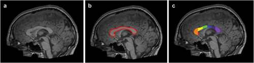
Hiess et al. (Hiess et al. 2015) also concluded that although there was no significant difference in the corpus callosum sub-regions between ASD and control participants, but the individuals facing ASD had increased intracranial volume. Intracranial volume (ICV) is used as an estimate of size of brain and brain regions/volumetric analysis (Nordenskjöld et al. 2013). Waiter et al. (Waiter et al. 2005) reported reduction in the size of splenium and isthmus and Chung et al. (Chung, et al., 2004) also found diminution in the area of splenium, genu and rostrum of corpus callosum in ASD. Whereas, splenium, isthmus, genu and rostrum are regional subdivisions of the corpus callosum based on Witelson et al. (Witelson 1989) and Venkatasubramanian et al. (Venkatasubramanian et al. 2007) studies. Refer Figure 2 for pictorial representation of different segmented sub-regions of corpus callosum. Motivation of using subdivisions of the corpus callosum and intracranial brain volume as feature vector (refer Section 4.1.1 for discussion on feature vector) in this study study comes from the fact that in the reviewed literature these regions are usually considered important for detection of ASD.

Figure 2. An example of corpus callosum area segmentation. The figure shows example data for an individual facing ASD in the ABIDE study. Figure A represents 3D volumetric T1-weighted MRI scan. Figure B represents segmentation of corpus callosum in red. Figure C represents the further division of corpus callosum according to the Witelson scheme (Witelson 1989). The regions W1(rostrum), W2(genu), W3(anterior body), W4(mid-body), W5(posterior body), W6(isthmus), and W7(splenium) are shown in red, orange, yellow, green, blue, purple, and light purple (Kucharsky Hiess et al. 2015).

Next section presents all the details related to the ABIDE database and also explains preprocessing procedure.

Database

This study is performed using structural MRI (s-MRI) scans from the Autism Brain Imaging Data Exchange (ABIDE-I) dataset (http://fcon_1000.projects.nitrc.org/indi/abide/abide_I.html). ABIDE is an online sharing consortium that provides imaging data of ASD and control participants with their phenotypic information (Di Martino et al. 2014). The ABIDE-I dataset consists of 17 international sites, with total of 1112 subjects or samples, that includes (539 autism cases and 573 healthy control participants). According to Health Insurance Portability and Accountability Act (HIPAA) (Act 1996) guidelines, the identity of individuals participated in ABIDE database recording was not disclosed. Table 1 shows image acquisition parameters for structural MRI (s-MRI) scans for each site in ABIDE study.

Table 1. Structural MRI acquisition parameters for each site in the ABIDE database (Kucharsky Hiess et al. 2015)

Site	Typical controls (m/f)	Autism Spectrum disorder (m/f)	Image acquisition	Make model	Voxel size ($m{m}^3$)	Flip angle (deg)	TR (ms)	TE (ms)	T1 (ms)	Bandwidth (Hz/Px)
CALTECH ${ }^a$	15/4	15/4	3D MPRAGE	Siemens Magnetom (Trio Trim)	1	10	1590	2.73	800	200
CMU ${ }^b$	10/3	11/3	3D MPRAGE	Siemens Magnetom (Verio)	1	8	1870	2.48	1100	170
KKI ${ }^c$	25/8	18/4	3D FFE	Philips (Achieva)	1	8	8	3.7	843	191.5
MAXMUN ${ }^d$	29/4	21/3	3D MPRAGE	Siemens Magnetom (Verio)	1	9	1800	3.06	900	230
NYU ${ }^e$	79/26	68/11	3D MPRAGE	Siemens Magnetom (Allegra)	$1.3\times 1.3$	7	2530	3.25	1100	200
OLIN ${ }^f$	13/3	18/2	3D MPRAGE	Siemens Magnetom (Allegra)	1	8	2500	2.74	900	190
OHSU ${ }^g$	15/0	15/0	3D MPRAGE	Siemens Magnetom (Trio Trim)	1	10	2300	3.58	900	180
SDSU ${ }^h$	16/6	13/1	3D SPGR	GE (MR750)	1	45	11.08	4.3	NA	NA
SBL ${ }^i$	15/0	15/0	3D FFE	Philips (Intera)	1	8	9	3.5	1000	191.5
STANFORD ${ }^j$	16/4	16/4	3D SPGR	GE (Signa)	$0.86\times 1.5\times 0.86$	15	8.4	1.8	NA	NA
TRINITY ${ }^k$	25/0	24/0	3D FFE	Philips (Achieva)	1	8	8.5	3.9	1060.17	178.7
UCLA_1 ${ }^l$	29/4	42/7	3D MPRAGE	Siemens Magnetom (Trio Trim)	$1\times 1\times 1.2$	9	2300	2.84	853	240
UCLA_2 ${ }^m$	12/2	13/0	3D MPRAGE	Siemens Magnetom (Trio Trim)	$1\times 1\times 1.2$	9	2300	2.84	853	240
LEUVEN_1 ${ }^n$	15/0	14/0	3D FFE	Philiphs (Intera)	$0.98\times 0.98\times 1.2$	8	9.6	4.6	885.145	135.4
LEUVEN_2 ${ }^o$	15/5	12/3	3D FFE	Philiphs (Intera)	$0.98\times 0.98\times 1.2$	8	9.6	4.6	885.145	135.4
UM_1 ${ }^p$	38/17	46/9	3D SPGR	GE (Signa)	$1.2\times 1\times 1$	15	250	1.8	500	15.63
UM_2 ${ }^q$	21/1	12/1	3D SPGR	GE (Signa)	$1\times 1\times 1.2$	15	250	1.8	500	15.63
PITT ${ }^r$	23/4	26/4	3D MPRAGE	Siemens Magnetom (Allegra)	$1.1\times 1.1\times 1.1$	7	2100	3.93	1000	130
USM ${ }^s$	43/0	58/0	3D MPRAGE	Siemens Magnetom (Trio Trim)	$1\times 1\times 1.2$	9	2300	2.91	900	240
YALE ${ }^t$	20/8	20/8	3D MPRAGE	Siemens Magnetom (Trio Trim)	1	9	1230	1.73	624	320

${ }^a$ California Institute of Technology

${ }^b$ Carnegie Mellon University

${ }^c$ Kennedy Krieger Institute, Baltimore

${ }^d$ Ludwig Maximilians University, Munich

${ }^e$ NYU Langone Medical Center, New York

${ }^f$ Olin, Institute of Living, Hartford Hospital

${ }^g$ Oregon Health and Science University

${ }^h$ San Diego State University

${ }^i$ Social Brain Lab BCN NIC UMC Groningen and Netherlands Institute for Neurosciences

${ }^j$ Stanford University

${ }^k$ Trinity Center for Health Sciences

${ }^{l,m}$ University of California, Los Angeles

${ }^{n,o}$ University of Leuven

${ }^{p,q}$ University of Michigan

${ }^r$ University of Pittsburgh School of Medicine

${ }^s$ University of Utah School of Medicine

${ }^t$ Child Study Center, Yale University

We used same features as used in the study of Hiess et al. (Kucharsky Hiess et al. 2015). Next, we will explain preprocessing done by Hiess et al. on T1-weighted MRI scans from ABIDE dataset to calculate different parameters and regions of corpus callosum and brain volume.

Preprocessing

Corpus callosum area, its sub-regions and intracranial volume were calculated using different softwares. These softwares are as follows:

1. yuki (Ardekani 2013)

2. fsl (https://fsl.fmrib.ox.ac.uk/fsl/fslwiki/)

3. itksnap (Yushkevich et al. 2006)

4. brainwash (https://www.nitrc.org/projects/art)

The corpus callosum have a central function in integrating information and mediating behaviors (Hinkley et al. 2012). The corpus callosum consists of approximately 200 million fibers of varying diameters and is the largest inter-hemispheric joint of the human brain (Tomasch 1954). Whereas, intracranial volume (ICV) is used as an estimate of size of brain and brain regions/volumetric analysis (Nordenskjöld et al. 2013).

The corpus callosum area for each participant was segmented using “yuki” software (Ardekani 2013). The corpus callosum was automatically divided into its subregions using the Witelson scheme (Witelson 1989). An example of corpus callosum segmentation is shown in Figure 2. Each segmentation was inspected visually and corrected necessarily using the “ITK-SNAP” (Yushkevich et al. 2006) software package. The inspection and correction procedure was performed by two readers. Due to minor manual correction in corpus callosum segmentation for some MRI scans, statistical equivalence analysis and intra-class correlation were calculated to measure corpus callosum area by both readers.

The total intracranial brain volume (Malone et al. 2015) of each participant was measured by using software tool “brainwash.” “Automatic Registration Toolbox” (www.nitrc.org/projects/art) $\mathrm{\_}$ a feature in brainwash was used to extract intracranial brain volume. The brainwash method uses non-linear transformation to estimate intracranial regions by mapping the co-registered labels (pre-labeled intracranial regions) to participant’s MRI scan. The voxel-voting scheme (Manjón and Coupé 2016) is used to classify each voxel in the participant MRI as intracranial or not. Each brain segmentation was visually inspected to ensure accurate segmentation. Some of cases where segmentation were not performed accurately, following additional steps were taken in order to process it:

1. In some cases where brain segmentation was not achieved correctly, the brainwash method was executed again with same site of preprocessed MRI scan that had error free brain segmentation.

2. The brainwash software automatically identifies the coordinates of anterior and posterior commissure. In some cases, these points were not correctly identified. In such cases, they were identified manually and entered in the software.

3. A “region-based snakes” feature implemented in “ITK-SNAP” (Yushkevich et al. 2006) software package was used for minor correction of intracranial volume segmentation error manually.

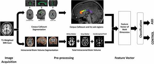
Figure 3 presents schematic overview of the proposed framework. It shows how T1-weighted MRI scans is transformed into feature vector of M x N dimension, where M denotes the total number of samples and N denotes total number of features in the feature vector. Where features are measurable attribute of the data (Bishop 2006). Then, these features are used for training model that detects ASD.

Figure 3. Schematic overview of the proposed framework.

Experiments and Results

Conventional Machine Learning Methods

In every machine learning problem before application of any machine learning method, selection of useful set of features or feature vector is an important task. The optimal features extracted from dataset minimizes within-class variations (ASD vs control individuals) while maximizes between class variations (Khan 2013c). Feature selection techniques are utilized to find optimal features by removing redundant or irrelevant features for a given task. The next subsection, Section 4.1.1, will present evaluated feature selection methods. Section 4.1.2 will discuss conventional machine learning methods used in this study, where conventional machine learning methods refer to methods other than recently popularized deep learning approach. Results from conventional machine learning methods are discussed in Section 4.1.3.

Feature Selection

As described above, we used same features as used in the study of Hiess et al. (Kucharsky Hiess et al. 2015). By using same features, we can robustly verify the relative strength or weakness of the proposed machine learning based framework as the study done by Hiess et al. does not employ machine learning. Hiess et al. have made preprocessed T1-weighted MRI scans data from ABIDE available for research (https://sites.google.com/site/hpardoe/cc_abide). Preprocessed data consists of parametric features of corpus callosum, its sub-regions and intracranial brain volume with label. In total, preprocessed data consists of 12 features from 1100 examples or samples each (12 x 1100). Statistical summary of preprocessed data is outlined in Table 2.

Table 2. Statistical summary of ABIDE preprocessed data

Class	Healthy Controls	Autism Spectrum Disorder
Number	571	529
Sex(m/f)	479/99	465/64
Age(years)	17.102 $\pm$ 7.726	17.082 $\pm$ 8.428
CC ${ }^a$_area ($m{m}^2$)	596.654 $\pm$ 102.93	596.908 $\pm$ 110.134
CC_perimeter ($m$)	196.405 $\pm$ 6.353	198.102 $\pm$ 17.265
CC_length ($m$)	70.583 $\pm$ 5.342	70.711 $\pm$ 5.671
CC_circularity	0.194 $\pm$ 0.020	0.191 $\pm$ 0.023
W1 ${ }^b$ (Rostrum) ($m$)	20.753 $\pm$ 14.264	25.899 $\pm$ 10.809
W2 ${ }^c$ (genu) ($m$)	128.789 $\pm$ 32.134	128.855 $\pm$ 33.704
W3 ${ }^d$ (anterior body) ($m$)	91.088 $\pm$ 19.212	91.734 $\pm$ 20.302
W4 ${ }^e$ (mid-body)($m$)	69.705 $\pm$ 13.351	69.345 $\pm$ 13.796
W5 ${ }^f$ (posterior body)($m$)	59.007 $\pm$ 11.698	59.454 $\pm$ 12.501
W6 ${ }^g$ (isthmus) ($m$)	51.843 $\pm$ 12.519	52.137 $\pm$ 13.313
W7 ${ }^h$ (splenium) ($m$)	175.471 $\pm$ 32.353	174.483 $\pm$ 34.562
Brain Volume ($m{m}^3$)	1,482,428.866 $\pm$ 150,985.323	1,504,247.415 $\pm$ 170,357.180

${ }^a$ CC = corpus callosum

${ }^{b,c,d,e,f,g,h}$ Witelson’s (Witelson 1989) sub-regions of the corpus callosum

Selection of useful subset of features to extract meaningful results by eliminating redundant feature is very comprehensive and recursive task. To enhance computational simplicity, reduce complexity and improve performance of machine learning algorithms, different feature selection techniques are applied on the preprocessed ABIDE dataset. In the literature, usually entropy or correlation based methods are used for feature selection. Thus, we have also employed state-of-the-art methods based on entropy and correlation to select features that minimizes within-class variations (ASD vs control individuals) while maximizes between class variations. Methods evaluated in this study are explained below:

Information Gain

Information gain $(IG)$ is a feature selection technique that measures how much information a feature provides for the corresponding class. It measures information in the form of entropy. Entropy is defined as probabilistic measure of impurity, disorder or uncertainty in feature (Quinlan 1986). Therefore, a feature with reduced entropy value intends to give more information and considered as more relevant. For a given set of $S_N$ training examples, $n_i$, the vector of $i^{th}$ feature in this set, $\frac{|S_{ni=v}|}{|S_N|}$, the fraction of the examples of $i^{th}$ feature with value $v$, the following equation is mathematically denoted:

(1) $IG(S_N,n_i)=H(S_N)-\sum _{v=values(n_i)}^{\frac{|S_{n_i=v}|}{|S_N|}}H(S_{n_i=v})$(1)

with entropy

(2) $H(S)=-p_{+}(S){log}_2{p}_{+}(S)-p_{-}(S){log}_2{p}_{-}(S)$(2)

$where;$

$p_{\pm }(S)$ is the probability of the training sample in dataset $S$ belonging to corresponding positive and negative class, respectively.

Information Gain Ratio

Information gain $(IG)$ is biased in selecting features with larger values (Yu and Liu 2003). The information gain ratio is modified version of information gain that reduces its bias. It is calculated as the ratio of information gain and intrinsic value (Kononenko and Hong 1997). The intrinsic value $(IV)$ is additional calculation of entropy. For a given set of features $Feat$, of all training examples $Ex$, with $values(x,f)$, where $x$ $\in$ $Ex$ defines the specific example $x$ with feature value $f$ $\in$ $Feat$. The $values(f)$ function denotes the set of all possible values of features $f$ $\in$ $Feat$. The information gain ratio $IGR(Ex,f)$ for a feature $f$ $\in$ $Feat$ is mathematically denoted as

(3) $IGR(Ex,f)=\frac{IG(Ex,f)}{IV}$(3)

with intrinsic value $(IV)$

(4) $IV(Ex,f)=\sum _{v\epsilon values(f)}\left(\frac{\left|x\in Ex\right|values(x,f)=v|}{\left|Ex\right|}\hspace{0.17em}\right).{log}_2\left(\frac{\left|x\in Ex\right|values(x,f)=v|}{\left|Ex\right|}\right)$(4)

Chi-Square Method

The Chi-Square (${\chi }^2$) is correlation based feature selection method (also known as the Pearson Chi-Square test), which calculates the dependencies of two independent variables, where two variables $A$ and $B$ are defined as independent, if $P(AB)=P(A)P(B)$, or equivalent, $P(A|B)=P(A)$ and $P(B|A)=P(B)$. In terms of machine learning, two variables are the occurrence of the features and class label (Doshi 2014). Chi square method calculates the correlation strength of each feature by calculating statistical value represented by the following expression:

(5) ${\chi }^2=\sum _{i=1}^n\left(\begin{array}{c}\frac{E_i-O_i}{E_i}\end{array}\right)$(5)

$where$

(${\chi }^2$) is the chi-square statistic, $O$ is the actual value of $i$ feature, and $E$ is the expected value of $i$ feature.

Symmetrical Uncertainty

Symmetrical Uncertainty (SU) is referred as relevance indexing or scoring (Brown et al. 2012) method which is used to find the relationship between a feature and class label. It normalizes the value of features within the range of [0, 1], where 1 indicates that feature and target class are strongly correlated and 0 indicates no relationship between them (Peng, Long, and Ding 2005). For a class label $Y$, the symmetrical uncertainty for set of features $X$ is mathematically denoted as

(6) $SU(X,Y)=\left[\begin{array}{c}\frac{2\ast IG(X,Y)}{H(X)+H(Y)}\end{array}\right]$(6)

$where;$

$IG(X,Y)$ represents information gain, and $H$ represents entropy, respectively.

All four methods (information gain, information gain ratio, chi-square and symmetrical uncertainty) calculate the value/importance/weight of each feature for a given task. The weight of each feature is calculated with respect to class label and feature value calculated by each method. The higher the weight of feature, the more relevant it is considered. The weight of each feature is normalized between in the range of [0, 1]. The results of each feature selection method is shown in Figure 4.

Figure 4. Results of entropy and correlation based feature selection methods. All features are represented with their corresponding weights. A represents the result of information gain. B represents the result of information gain ratio. C represents the result of chi-square method. D represents the result of symmetrical uncertainty.

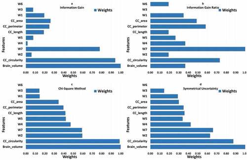
Figure 4 presents result of feature selection study. First two graphs show weights of different features calculated from entropy based methods i.e. information gain and information gain ratio. Last two graphs present feature weights obtained from correlation based methods i.e. chi-square and symmetrical uncertainty. Result of information gain ratio differs from information gain but in both the methods $W7$ and $CC\mathrm{\_}circularity$ emerged as most important features. Results from correlation based methods i.e. chi-square and symmetrical uncertainty are almost similar with little differences. $brain\mathrm{\_}volume$, $W7$, $W2$ and $CC\mathrm{\_}circularity$ emerged as the most discriminant features.

It is important to highlight that feature(s) that give more discriminant information in our study are comparable with features identified in study by Hiess et al. (Kucharsky Hiess et al. 2015). Hiess et al. (Kucharsky Hiess et al. 2015) concluded that $brain\mathrm{\_}volume$ and corpus callosum area are two important features used to discriminate ASD and control in ABIDE dataset. In our study, we also concluded that $brain\mathrm{\_}volume$ and different sub-regions of corpus callosum, i.e. genu, mid-body and splenium, labeled as $W2$, $W4$ and $W7$ are most discriminant features. As a matter of fact, results from correlation based methods, i.e. chi-square and symmetrical uncertainty, are comparable with the results presented by Hiess et al. (Kucharsky Hiess et al. 2015).

In our proposed framework, we have applied threshold on results obtained from the feature(s) selection method to select a subset of features that reduce computational complexity and improve performance of machine learning algorithms. We performed experiments with different threshold values and empirically found that average classification accuracy (detection of ASD) obtained on subset of features from chi-square method at threshold value $p=0.4$ is highest.

Final feature vector deduced in this study includes $Brain\mathrm{\_}volume$, $CC\mathrm{\_}circularity$, $CC\mathrm{\_}length$, $W2(genu)$, $W4(mid-body)$, $W5(posterior-body)$ and $W7(splenium)$, where $CC$ = corpus callosum. Average classification accuracy, after application of conventional machine learning methods, with and without feature selection method is presented in Table 3. It can be observed from table that training classifier on subset of discriminant features gives better result not only in terms of computational complexity by also in terms of average classification accuracy.

Table 3. Average classifiers accuracy with and without feature selection

	Without Feature Selection	With Feature Selection
	Average Accuracy using	Average Accuracy using	Average Accuracy using
	leave-one-site-out classification	leave-one-site-out classification	5-fold cross-validation
Linear Discriminant Analysis (LDA)	55.45%	56.21%	55.93%
Support Vector Machine (SVM)	51.34%	51.34%	52.2%
Random Forest (RF)	53.9%	54.61%	54.79%
Multi-Layer Perceptron (MLP)	52.8%	56.26%	54.98%
K-Nearest Neighbor (KNN)	48.74%	52.16%	51%

Next subsection, Subsection 4.1.2, discusses conventional machine learning methods evaluated in this study.

Utilized Conventional Machine Learning Methods

Classification is a process of searching patterns/learning pattern/concept from a given dataset or examples and predicting its class (Bishop 2006). For automatic detection of ASD from preprocessed ABIDE dataset (features selected by feature selection algorithm, refer Section 4.1.1), we have evaluated below mentioned state-of-the-art conventional machine learning classifiers:

1. Linear Discriminant Analysis (LDA)

2. Support Vector Machine (SVM) with radial basis function (rbf) Kernel

3. Random Forest (RF) of 10 trees

4. Multi-Layer Perceptron (MLP)

5. K-Nearest Neighbor (KNN) with $K$ = 3

We chose classifiers from diverse categories. For example, K-Nearest Neighbor (KNN) is nonparametric instance based learner, Support Vector Machine (SVM) is large margin classifier that theorizes to map data to higher dimensional space for better classification, and Random Forest (RF) is tree based classifier that breaks the set of samples into a set of covering decision rules while Multilayer Perceptron (MLP) is motivated by human brain anatomy. The above mentioned classifiers are briefly explained below.

Linear Discriminant Analysis (LDA)

LDA is a statistical method that finds linear combination of features, which separates the dataset into their corresponding classes. The resulting combination is used as linear classifier (Jain and Huang 2004). LDA maximizes the linear separability by maximizing the ratio of between-class variance to the within-class variance for any particular dataset. Let ${\omega }_1,{\omega }_2,..,{\omega }_L$ and $N_1,N_2,..,N_L$ be the classes and number of exampleset in each class, respectively. Let $M_1,M_2\dots ,M_L$ and $M$ be the means of the classes and grand mean, respectively. Then, the within and between class scatter matrices $S_w$ and $S_b$ are defined as

(7) $S_w=\sum _{i=1}^{L}P({\omega }_i)\sum _i=\sum _{i=1}^{L}P({\omega }_i)E\{[X-M_i][X-M_i{]}^t|\omega \}$(7)

(8) $S_b=\sum _{i=1}^{L}P({\omega }_i)\{[M_i-M][M_i-M{]}^t\}$(8)

$where;$

$(P_{{\omega }_i})$ is the prior probability and ${\sum }_i$ represents covariance matrix of class ${\omega }_i$.

Support Vector Machine (SVM)

The SVM classifier segregates samples into corresponding classes by constructing decision boundaries known as hyperplanes (Vapnik 2013). It implicitly maps the dataset into higher dimensional feature space and constructs a linear separable line with maximal marginal distance to separates hyperplane in higher dimensional space. For a training set of examples {$(x_i,y_i),i=1\dots ,l$} where $x_i$ $\in$ ${\mathrm{\Re }}^n$ and $y_i$ $\in$ $\{$ −1, 1 $\}$, a new test example $x$ is classified by the following function:

(9) $f\left(x\right)=sgn(\sum _{i=1}^l{\alpha }_i{y}_{i}K(x_i,x)+b)$(9)

$where;$

${\alpha }_i$ are Langrange multipliers of a dual optimization problem separating two hyperplanes, $K(.,.)$ is a kernel function, and $b$ is the threshold parameter of the hyperplane.

Random Forest (RF)

Random Forest belongs to the family of decision tree, capable of performing classification and regression tasks. A classification tree is composed of nodes and branches that break the set of samples into a set of covering decision rules (Mitchell 1997). RF is an ensemble tree classifier consisting of many correlated decision trees and its output is the mode of class’s output by individual decision tree.

Multilayer Perceptron (MLP)

MLP belongs to the family of neural-nets, which consists of interconnected group of artificial neurons called nodes and connections for processing information called edges (Jain, Mao, and Moidin Mohiuddin 1996). A neural network consists of an input, hidden and output layer. The input layer transmits inputs in form of feature vector with a weighted value to hidden layer. The hidden layer, is composed with activation units or transfer function (Gardner and Dorling 1998), carries the features vector from first layer with weighted value and performs some calculations as output. The output layer is made up of single activation units, carrying weighted output of hidden layer and predicts the corresponding class. An example of MLP with 2 hidden layer is shown in Figure 5. Multilayer perceptron is described as fully connected, with each node connected to every node in the next and previous layer. MLP utilizes the functionality of back-propagation (Hecht-Nielsen 1992) during training to reduce the error function. The error is reduced by updating weight values in each layer. For a training set of examples {$X=(x_1,x_2,x_3,\dots .,x_m)$} and output $y$ $\in$ $\{$ 0, 1 $\}$, a new test example $x$ is classified by the following function:

(10) $y\left(x\right)=f(\sum _{j=1}^n{x}_j{w}_j+b)$(10)

$where;$

Figure 5. An architecture of Multilayer Perceptron (MLP).

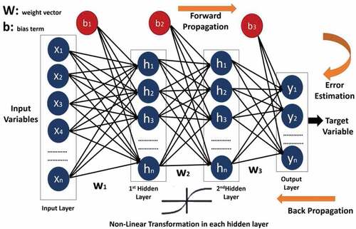
$f$ is non-linear activation function, $w_j$ is weight multiplied by inputs in each layer $j$, and $b$ is bias term.

K-Nearest Neighbor (KNN)

KNN is an instance based non-parametric classifier which is able to find number of training samples closest to new example based on target function (Khan, 2013c; Acuna and Rodriguez 2004). Based upon the value of targeted function, it infers the value of output class. The probability of an unknown sample $q$ belonging to class $y$ can be calculated as follows:

(11) $p(y|q)=\frac{\sum _{k\in K}{W}_k{.1}_{(k_y=y)}}{\sum _{k\in K}{W}_k}$(11)

(12) $W_k=\frac{1}{d(k,q)}$(12)

$where;$

$K$ is the set of nearest neighbors, $k_y$ is the class of $k$, and $d(k,q)$ is the Euclidean distance of $k$ from $q$.

Results and Evaluation

We chose to evaluate the performance of our framework in the same way, as evaluation criteria proposed by Heinsfeldl et al. (Heinsfeld et al. 2018). Heinsfeldl et al. evaluated the performance of their framework on the basis of $k$-fold cross validation and leave-one-site-out classification schemes (Bishop 2006). We have also evaluated results of above mentioned classifiers based on these schemes.

k-Fold Cross Validation Scheme

Cross validation is statistical technique for evaluating and comparing learning algorithms by dividing the dataset into two segments: one used to learn or train the model and other used to validate the model (Kohavi . 1995). In $k$-fold cross validation schema, dataset is segmented into $k$ equally sized portions, segments or folds. Subsequently, $k$ iterations of learning and validation are performed, within each iteration $(k-1)$ folds are used for learning and a different fold of data is used for validation (Bishop 2006). Upon completion of $k$ folds, performance of an algorithm is calculated by averaging values of evaluation metric i.e. accuracy of each fold.

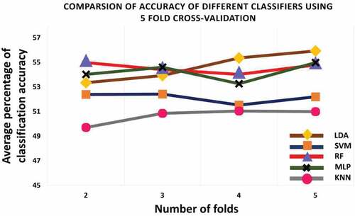
All the studied classifiers are evaluated on 5-fold cross validation scheme. The dataset is divided into 5 segments of equal portions. In 5-fold cross validation, 4 segments of data are used for training purpose and the other one portion is used for testing purpose.

Figure 6 presents average ASD recognition accuracy achieved by studied classifier using 5-fold cross validation scheme on preprocessed ABIDE data (features selected by feature selection algorithm, refer Section 4.1.1).The result shows that the overall accuracy of all classifiers increases with the number of folds. Linear discriminant analysis (LDA), Support Vector Machine (SVM), Random Forest (RF), Multi-layer Perceptron (MLP) and K-nearest neighbor (KNN) achieved an average accuracy of 55.93%, 52.20%, 54.79%, 54.98% and 51.00%, respectively. The result is also reported in Table 3.

Figure 6. Results of the 5-fold cross-validation scheme.

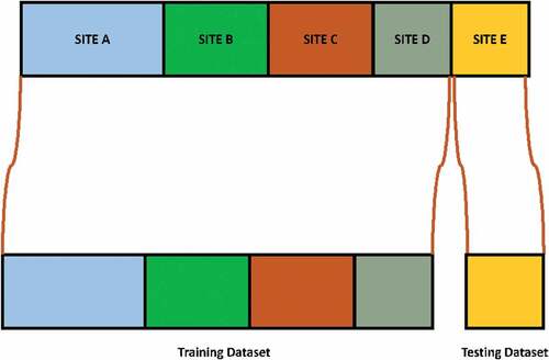
Leave-one-site-out Classification Scheme

In this classification validation scheme data from one site is used for testing purpose to evaluate the performance of model and rest of data from other sites is used for training purpose. This procedure is represented in Figure 7.

Figure 7. Schematic overview of the leave-one-site-out classification scheme.

The framework achieved an average accuracy of 56.21%, 51.34%, 54.61%, 56.26% and 52.16% for linear discriminant analysis (LDA), Support Vector Machine (SVM), Random Forest (RF), Multi-layer Perceptron (MLP) and K-nearest neighbor (KNN) for ASD identification using leave-one-site-out classification scheme. Results are tabulated in Table 3.

Figure 8 presents recognition result for each site using leave-one-site-out classification method. It is interesting to observe that for all sites, maximum ASD classification accuracy is achieved for USM site data, with accuracy of 79.21% by 3-NN classifier. The second highest accuracy is achieved by LDA, with accuracy of 76.32% on CALTECH site data. This result is consistent with the result obtained by Heinsfeldl et al. (Heinsfeld et al. 2018).

Figure 8. Results of the leave-one-site-out classification scheme.

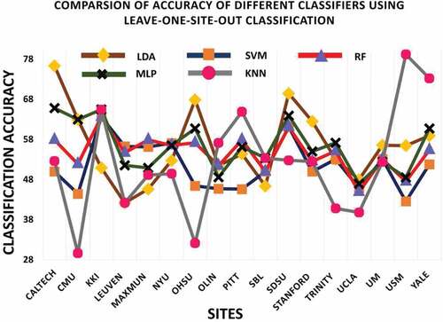
The results of leave-one-site-out classification of all classifiers shows variations across different sites. The result suggests that this variation could be due to change in number of samples size used for training phase. Furthermore, there is variability in data across different sites. Refer Table 1 for structural MRI acquisition parameters used across sites in the ABIDE dataset (Kucharsky Hiess et al. 2015).

Transfer Learning Based Approach

Results obtained with conventional machine learning algorithms with and without feature selection method are presented in Section 4.1.3. It can be observed that average recognition accuracy for autism detection on ABIDE dataset remains between the range of 52% and 55% for different conventional machine learning algorithms; refer Table 3. In order achieve better recognition accuracy and to test the potential of latest machine learning technique, i.e. deep learning (LeCun, Bengio, and Hinton 2015), we employed the transfer learning approach using the VGG16 model (Simonyan and Zisserman 2014).

Generally, training and test data are drawn from same distribution in machine learning algorithms. On the contrary, transfer learning allows distributions used in training and testing to be different (Pan and Yang 2010). Motivation for employing transfer learning approach comes from the fact that training deep learning network from the scratch requires large amount of data (LeCun, Bengio, and Hinton 2015), but in our case, the ABIDE dataset (Di Martino et al. 2014) contains labeled samples from 1112 subjects (539 autism cases and 573 healthy control participants). Transfer learning allows partial re-training of already trained model (re-training usually last layer) (Pan and Yang 2010) while keeping all other layers (trained weights) in the model intact, which are trained on millions of examples for semantically similar task. We used transfer learning approach in our study as we wanted to benefit from deep learning model that has achieved high accuracy on visual recognition tasks, i.e. ImageNet Large-Scale Visual Recognition Challenge (ILSVRC) (Russakovsky et al. 2015), and is available for research purposes.

Few of the well known deep learning architectures that emerged from ILSVRC are GoogleNet (a.k.a. Inception V1) from Google (Szegedy et al. 2015) and VGGNet by Simonyan and Zisserman (Simonyan and Zisserman 2014). Both of these architectures are from the family of Convolutional Neural Networks or CNN as they employ convolution operations to analyze visual input i.e. images. We chose to work with VGGNet, which consists of 16 convolutional layers (VGG16) (Simonyan and Zisserman 2014). It is one of the most appealing framework because of its uniform architecture and its robustness for visual recognition tasks, refer Figure 9. It’s pre-trained model is freely available for research purpose, thus making a good choice for transfer learning.

Figure 9. An illustration of VGG16 architecture (Simonyan and Zisserman 2014).

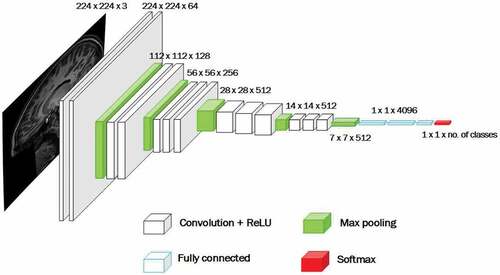
VGG16 architecture (refer Figure 9) takes image of 224 × 224 with the receptive field size of 3 x 3, convolution stride is 1 pixel and padding is 1 (for receptive field of 3 × 3). It uses rectified linear unit (ReLU) (Nair and Hinton 2010) as activation function. Classification is done using softmax classification layer with $x$ units (representing $x$ classes/$x$ classes to recognize). Other layers are Convolution layer and Feature Pooling layer. Convolution layer use filters which are convolved with the input image to produce activation or feature maps. Feature Pooling layer is used in the architecture to reduce size of the image representation, to make the computation efficient and control over-fitting.

Results

As mentioned earlier, this study is performed using structural MRI (s-MRI) scans from Autism Brain Imaging Data Exchange (ABIDE-I) dataset (http://fcon_1000.projects.nitrc.org/indi/abide/abide_I.html) (Di Martino et al. 2014). ABIDE-I dataset consists of 17 international sites, with total of 1112 subjects or samples, that includes (539 autism cases and 573 healthy control participants).

MRI scans in the dataset ABIDE-I are provided in the Neuroimaging Informatics Technology Initiative (nifti) file format (Cox et al. 2003), where images represent the projection of an anatomical volume onto an image plane. Initially, all anatomical scans were converted from nifti to Tagged Image File Format, i.e. TIFF or TIF, a compression less format (Guarneri, Vaccaro, and Guarneri 2008), which created a dataset of $\approx$ 200k tif images. But we did not use all tif images for transfer learning as beginning and trailing portion of images extracted from individual scans contains clipped/cropped portion of region of interest i.e. corpus callosum. Thus, we were left with $\approx$ 100k tif images with visibly complete portion of corpus callosum.

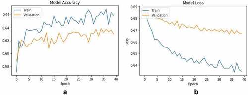
For transfer learning, VGGNet which consists of 16 convolutional layers (VGG16) was used (Simonyan and Zisserman 2014) (refer Section 4.2 for explanation of VGG16 architecture). Last fully connected dense layer of VGG16 pre-trained model was replaced and re-trained with extracted images from ABIDE-I dataset. We trained last dense layer with images using softmax activation function and ADAM optimizer (Kingma and Ba 2014) with learning rate of 0.01.

80% of the tif images extracted from MRI scans were used for training, while for validation, 20% of the frames were used. With the above mentioned parameters, the proposed transfer learning approach achieved an autism detection accuracy of 66%. Model accuracy and loss curves are shown in Figure 10. In comparison with conventional machine learning methods (refer Table 3 for results obtained using different conventional machine learning methods), the transfer learning approach gained around 10% in ASD detection.

Figure 10. Transfer learning results using VGG16 architecture: (A) training accuracy vs Validation accuracy and (B) training loss vs validation loss.

Conclusion and Future Work

Our research study shows the potential of machine learning (conventional and deep learning) algorithms for development of neuroimaging data understanding. We showed how machine learning algorithms can be applied to structural MRI data for automatic detection of individuals facing Autism Spectrum Disorder (ASD).

Although the achieved recognition rate is in the range of 55% – 65%, but still in the absence of biomarkers, such algorithms can assist clinicians in early detection of ASD. Second, it is known that studies that combine machine learning with brain imaging data collected from multiple sites like ABIDE (Di Martino et al. 2014) to identify autism demonstrated that classification accuracy tends to decrease (Arbabshirani et al. 2017). In this study, we also observed the same trend.

Main conclusions drawn from this study are as follows:

– Machine learning algorithms applied to brain anatomical scans can help in automatic detection of ASD. Features extracted from corpus callosum and intracranial brain regions present significant discriminative information to classify individual facing ASD from control subgroup.

– Feature selection/weighting methods help build a robust classifier for automatic detection of ASD. These methods not only help framework in terms of reducing computational complexity but also in terms of getting better average classification accuracy.

– We also provided automatic ASD detection results using Convolutional Neural Networks (CNN) via the transfer learning approach. This will help readers to understand the benefits and bottlenecks of the using deep learning/CNN approach for analyzing neuroimaging data, which is difficult to record in large enough quantity for deep learning.

– To enhance the recognition results of the proposed framework, it is recommended to use a multimodal system. In addition to neuroimaging data other modalities, i.e. EEG, speech or kinesthetic can be analyzed simultaneously to achieve better recognition of ASD.

Results obtained using Convolutional Neural Networks (CNN)/deep learning are promising. One of the challenge to fully utilize learning/data modeling capabilities of CNN is the use of large database to learn concept (LeCun, Bengio, and Hinton 2015; Zhou, Bin, and Zhenguo 2018), making it impractical for applications where labeled data is hard to record. For clinical applications where getting data, specially neuroimaging data is difficult, and training of a deep learning algorithm poses challenge. One of the solution to counter this problem is to propose a hybrid approach, where data modeling capabilities of conventional machine learning algorithms (which can learn the concept on small data as well) are combined with deep learning.

In order to bridge down the gap between neuroscience and computer science researchers, we emphasize and encourage the scientific community to share the database and results for automatic identification of psychological ailments.

Compliance With Ethical Standards

Authors have no conflict of interest. This article does not contain any studies with human participants performed by any of the authors.

Disclosure Statement

No potential conflict of interest was reported by the author(s).

Notes

1. Clinical information such as age, sex and ethnicity

References

- Act, A. 1996. Health insurance portability and accountability act of 1996. Public Law 104:369.
- Acuna, E., and C. Rodriguez. 2004. The treatment of missing values and its effect on classifier accuracy. In Classification, clustering, and data mining applications, 639–401. Berlin, Heidelberg: Springer.
- Arbabshirani, M. R., S. Plis, J. Sui, and V. D. Calhoun. 2017. Single subject prediction of brain disorders in neuroimaging: Promises and pitfalls. NeuroImage 145 (Pt B):137–65. doi:10.1016/j.neuroimage.2016.02.079.
- Ardekani, B. A. 2013. Yuki module of the automatic registration toolbox (art) for corpus callosum segmentation. Google Scholar.
- Barkley, R. A., and K. R. Murphy. 1998. Attention-deficit hyperactivity disorder: A clinical workbook. New York: Guilford Press.
- Baron-Cohen, S., S. Wheelwright, R. Skinner, J. Martin, and E. Clubley. 2001. The autism-spectrum quotient (aq): Evidence from asperger syndrome/high-functioning autism, malesand females, scientists and mathematicians. Journal of Autism and Developmental Disorders 31 (1):05–17. doi:10.1023/A:1005653411471.
- Bauer, A. J., and M. A. Just. 2015. Monitoring the growth of the neural representations of new animal concepts. Human Brain Mapping 36 (8):3213–26. doi:10.1002/hbm.22842.
- Bellak, L. 1994. The schizophrenic syndrome and attention deficit disorder. Thesis, antithesis, and synthesis? The American Psychologist 49 (1):25–29. doi:10.1037/0003-066X.49.1.25.
- Bishop, C. 2006. Pattern Recognition and Machine Learning. New York: Springer-Verlag.
- Bourgeron, T. 2009. A synaptic trek to autism. Current Opinion in Neurobiology 7 (2):0231–34. doi:10.1016/j.conb.2009.06.003.
- Brown, G., A. Pocock, M.-J. Zhao, and L. Mikel. 2012. Conditional likelihood maximisation: A unifying framework for information theoretic feature selection. Journal of Machine Learning Research 130 (Jan):027–66.
- Buchweitz, A., S. V. Shinkareva, R. A. Mason, T. M. Mitchell, and M. A. Just. 2012. Identifying bilingual semantic neural representations across languages. Brain and Language 120 (3):282–89. doi:10.1016/j.bandl.2011.09.003.
- Budman, S. H., M. F. Hoyt, and S. Friedman. 1992. The first session in brief therapy. New York: Guilford Press.
- Buescher, A. V. S., Z. Cidav, M. Knapp, and D. S. Mandell. 2014. Costs of autism spectrum disorders in the United Kingdom and the United States. JAMA Pediatrics 168 (8):721–28. doi:10.1001/jamapediatrics.2014.210.
- Bullmore, E., and O. Sporns. 2009. Complex brain networks: Graph theoretical analysis of structural and functional systems. Nature Reviews. Neuroscience 10 (3):186. doi:10.1038/nrn2575.
- Cameron Craddock, R., and P. E. Holtzheimer III. 2009. Xiaoping P Hu, and Helen S Mayberg. Disease state prediction from resting state functional connectivity. Magnetic Resonance in Medicine: An Official Journal of the International Society for Magnetic Resonance in Medicine 47 (6):921–29. doi:10.1002/mrm.22159.
- Castillo, R. J., D. J. Carlat, T. Millon, C. M. Millon, S. Meagher, S. Grossman, R. Rowena, and J. Morrison, et al. American Psychiatric Association. 2007. Diagnostic and statistical manual of mental disorders. Washington, DC: American Psychiatric Association Press.
- Chandrashekar, G., and F. Sahin. 2014. A survey on feature selection methods. Computers & Electrical Engineering 40 (1):016–28. doi:10.1016/j.compeleceng.2013.11.024.
- Choi, H. 2017. Functional connectivity patterns of autism spectrum disorder identified by deep feature learning. connections 4:5.
- Chung, M. K., K. M. Dalton, A. L. Alexander, and R. J. Davidson. 2004. Less white matter concentration in autism: 2d voxel-based morphometry. Neuroimage 23 (1):242–51. doi:10.1016/j.neuroimage.2004.04.037.
- Cox, R. W., J. Ashburner, H. Breman, K. Fissell, C. Haselgrove, C. J. Holmes, J. L. Lancaster, D. E. Rex, S. M. Smith, and J. B. Woodward, et al. A (sort of) new image data format standard: NiFTI-1. In 10th Annual Meeting of Organisation of Human Brain Mapping Budapest, Hungary, 2003.
- Crenn, A., A. Meyer, H. Konik, R. A. Khan, and S. Bouakaz. 2020. Generic body expression recognition based on synthesis of realistic neutral motion. IEEE Access 8:207758–67. doi:10.1109/ACCESS.2020.3038473.
- Del Valle Rubido, M., J. T. McCracken, E. Hollander, F. Shic, J. Noeldeke, L. Boak, O. Khwaja, S. Sadikhov, P. Fontoura, and D. Umbricht. 2018. In search of biomarkers for autism spectrum disorder. Autism Research 11 (11):1567–79. doi:10.1002/aur.2026.
- Di Martino, A., C.-G. Yan, L. Qingyang, E. Denio, F. X. Castellanos, K. Alaerts, J. S. Anderson, M. Assaf, S. Y. Bookheimer, M. Dapretto, et al. 2014. The autism brain imaging data exchange: Towards a large-scale evaluation of the intrinsic brain architecture in autism. Molecular Psychiatry. 19(6):659. doi:10.1038/mp.2013.78.
- Doshi, M., and S. K. Chaturvedi. 2014. Correlation based feature selection (cfs) technique to predict student perfromance. International Journal of Computer Networks & Communications 6 (3):197. doi:10.5121/ijcnc.2014.6315.
- Erkan, U., and N. H. Dang. 2019. Thanh. Autism spectrum disorder detection with machine learning methods. Current Psychiatry Research and Reviews 150 (4):0297–308. 2666-0822/2666-0830. doi:10.2174/2666082215666191111121115.
- Gardner, M. W., and S. R. Dorling. 1998. Artificial neural networks (the multilayer perceptron)—a review of applications in the atmospheric sciences. Atmospheric Environment 32 (14–15):2627–36. doi:10.1016/S1352-2310(97)00447-0.
- Giedd, J. N. 2004. Structural magnetic resonance imaging of the adolescent brain. Annals of the New York Academy of Sciences 1021 (1):077–85. doi:10.1196/annals.1308.009.
- Greicius, M. D., B. H. Flores, V. Menon, G. H. Glover, H. B. Solvason, H. Kenna, A. L. Reiss, and A. F. Schatzberg. 2007. Resting-state functional connectivity in major depression: Abnormally increased contributions from subgenual cingulate cortex and thalamus. Biological Psychiatry 62 (5):429–37. doi:10.1016/j.biopsych.2006.09.020.
- Guarneri, F., M. Vaccaro, and C. Guarneri. 2008. Digital image compression in dermatology: Format comparison. Telemedicine and e-Health 14 (7):666–70. PMID: 18817495. doi:10.1089/tmj.2007.0119.
- Haxby, J. V., M. Ida Gobbini, M. L. Furey, A. Ishai, J. L. Schouten, and P. Pietrini. 2001. Distributed and overlapping representations of faces and objects in ventral temporal cortex. Science 293 (5539):2425–30. doi:10.1126/science.1063736.
- Hecht-Nielsen, R. 1992. Theory of the backpropagation neural network. In Neural networks for perception, 65–93. San Diego: Elsevier.
- Heinsfeld, A. S., A. R. Franco, R. Cameron Craddock, A. Buchweitz, and F. Meneguzzi. 2018. Identification of autism spectrum disorder using deep learning and the abide dataset. NeuroImage: Clinical 17:16–23. doi:10.1016/j.nicl.2017.08.017.
- Hinkley, L. B. N., E. J. Marco, A. M. Findlay, S. Honma, R. J. Jeremy, Z. Strominger, P. Bukshpun, M. Wakahiro, W. S. Brown, L. K. Paul, et al. 2012. The role of corpus callosum development in functional connectivity and cognitive processing. PLOS ONE 7 (8):1–17. doi:10.1371/journal.pone.0039804.
- Horlin, C., M. Falkmer, R. Parsons, M. A. Albrecht, T. Falkmer, and J. G. Mulle. 2014. The cost of autism spectrum disorders. PLoS One 9 (9):e106552. doi:10.1371/journal.pone.0106552.
- Huettel, S. A., A. W. Song, and G. McCarthy, et al. 2004. Functional magnetic resonance imaging, vol. 1. MA: Sinauer Associates Sunderland
- Jain, A. K., J. Mao, and K. Moidin Mohiuddin. 1996. Artificial neural networks: A tutorial. Computer 29 (3):031–44. doi:10.1109/2.485891.
- Jain, A., and J. Huang. Integrating independent components and linear discriminant analysis for gender classification. In Automatic Face and Gesture Recognition, 2004. Proceedings. Sixth IEEE International Conference on Seoul, South Korea, 159–63. IEEE, 2004.
- Jaliaawala, M. S., and R. A. Khan. 2019. Can autism be catered with artificial intelligence-assisted intervention technology? A comprehensive survey. Artificial Intelligence Review 53. 1039–1069.
- Just, M. A., V. L. Cherkassky, A. Buchweitz, T. A. Keller, T. M. Mitchell, and A. Sirigu. 2014. Identifying autism from neural representations of social interactions: Neurocognitive markers of autism. PloS One 9 (12):e113879. doi:10.1371/journal.pone.0113879.
- Kak, A. C., and M. Slaney. 1988. Principles of computerized tomographic imaging. New York: IEEE press.
- Kassam, K. S., A. R. Markey, V. L. Cherkassky, G. Loewenstein, M. A. Just, and M. Gray. 2013. Identifying emotions on the basis of neural activation. PloS One 8 (6):e66032. doi:10.1371/journal.pone.0066032.
- Khan, R. A., A. Crenn, A. Meyer, and S. Bouakaz. 2019a. A novel database of children’s spontaneous facial expressions (LIRIS-CSE). Image Vision Comput 83-84:61–69. doi:10.1016/j.imavis.2019.02.004.
- Khan, R. A., A. Meyer, H. Konik, and S. Bouakaz. Pain detection through shape and appearance features. In 2013 IEEE International Conference on Multimedia and Expo (ICME) San Jose, California, USA, 1–6, July 2013a. doi: 10.1109/ICME.2013.6607608.
- Khan, R. A., A. Meyer, H. Konik, and S. Bouakaz. 2013b. Framework for reliable, real-time facial expression recognition for low resolution images. Pattern Recognition Letters 34 (10):1159–68. doi:10.1016/j.patrec.2013.03.022.
- Khan, R. A., A. Meyer, H. Konik, and S. Bouakaz. 2019b, February. Saliency-based framework for facial expression recognition. Frontiers of Computer Science 13 (1):183–98. 2095-2236. doi:10.1007/s11704-017-6114-9.
- Khan, R. A. Detection of emotions from video in non-controlled environment. PhD thesis, LIRIS, Universite Claude Bernard Lyon1, France, 2013c.
- Kingma, D. P., and J. Ba. Adam: A method for stochastic optimization. CoRR, arXiv:1412.6980, 2014.
- Klin, A., F. R. Volkmar, and S. S. Sparrow. 2000. Asperger syndrome. New York: Guilford Press.
- Kohavi, R. A study of cross-validation and bootstrap for accuracy estimation and model selection. In International joint conference on Artificial intelligence Montreal, Canada, 14, 1137–45. , 1995.
- Kononenko, I., and S. J. Hong. 1997. Attribute selection for modelling. Future Generation Computer Systems 13 (2–3):181–95. doi:10.1016/S0167-739X(97)81974-7.
- Konukoglu, E., B. Glocker, D. Zikic, and A. Criminisi. Neighbourhood approximation forests. In International Conference on Medical Image Computing and Computer-Assisted Intervention Nice, France, 75–82. Springer, 2012.
- Koyamada, S., Y. Shikauchi, K. Nakae, M. Koyama, and S. Ishii. Deep learning of fmri big data: A novel approach to subject-transfer decoding. arXiv preprint arXiv:1502.00093, 2015.
- Kucharsky Hiess, R., R. Alter, S. Sojoudi, B. A. Ardekani, R. Kuzniecky, and H. R. Pardoe. 2015. Corpus callosum area and brain volume in autism spectrum disorder: Quantitative analysis of structural mri from the abide database. Journal of Autism and Developmental Disorders 45 (10):3107–14. doi:10.1007/s10803-015-2468-8.
- Kushki, A., E. Drumm, M. P. Mobarak, N. Tanel, A. Dupuis, T. Chau, and E. Anagnostou. 2013. Investigating the autonomic nervous system response to anxiety in children with autism spectrum disorders. PLoS One 8 (4):e59730. doi:10.1371/journal.pone.0059730.
- LeCun, Y., Y. Bengio, and G. Hinton. 2015. Deep learning. Nature 521 (7553):436–44. doi:10.1038/nature14539.
- Lei, Y., and H. Liu. 2003. Feature selection for high-dimensional data: A fast correlation-based filter solution. 856–63.
- Malone, I. B., K. K. Leung, S. Clegg, J. Barnes, J. L. Whitwell, J. Ashburner, N. C. Fox, and G. R. Ridgway. 2015. Accurate automatic estimation of total intracranial volume: A nuisance variable with less nuisance. Neuroimage 104:366–72. doi:10.1016/j.neuroimage.2014.09.034.
- Manjón, J. V., and P. Coupé. 2016. volbrain: An online mri brain volumetry system. Frontiers in Neuroinformatics 10:30. doi:10.3389/fninf.2016.00030.
- Mazumdar, P., G. Arru, and F. Battisti. 2021. Early detection of children with autism spectrum disorder based on visual exploration of images. Signal Processing: Image Communication 94: 0923-5965: 116184. doi:10.1016/j.image.2021.116184.
- McGuire, S. A., S. A. Wijtenburg, P. M. Sherman, L. M. Rowland, M. Ryan, J. H. Sladky, and P. V. Kochunov. 2017. Reproducibility of quantitative structural and physiological MRI measurements. Brain and Behavior 7 (9):e00759. doi:10.1002/brb3.759.
- Mitchell, T. M. 1997. Machine Learning. New York, United States: McGraw-Hill Series in Computer Science.
- Munir, R., and R. A. Khan. 2019. An extensive review on spectral imaging in biometric systems: Challenges & advancements. Journal of Visual Communication and Image Representation 65: 1047-3203: 102660. doi:10.1016/j.jvcir.2019.102660.
- Nair, V., and G. E. Hinton. Rectified linear units improve restricted boltzmann machines. In Proceedings of the 27th International Conference on International Conference on Machine Learning, ICML’10, 807–14, USA, 2010. Omnipress. 978-1-60558-907-7. http://dl.acm.org/citation.cfm?id=3104322.3104425
- Nazir, A., and R. A. Khan. 2021. A novel combinatorial optimization based feature selection method for network intrusion detection. Computers & Security 102: 0167-4048: 102164. doi:10.1016/j.cose.2020.102164.
- Nielsen, J. A., B. A. Zielinski, P. Thomas Fletcher, A. L. Alexander, N. Lange, E. D. Bigler, J. E. Lainhart, and J. S. Anderson. 2013. Multisite functional connectivity mri classification of autism: Abide results. Frontiers in Human Neuroscience 7:599. doi:10.3389/fnhum.2013.00599.
- Nordenskjöld, R., F. Malmberg, E.-M. Larsson, S. J. Andrew Simmons, L. L. Brooks, H. Ahlström, L. Johansson, J. Kullberg, and J. Kullberg. 2013. Intracranial volume estimated with commonly used methods could introduce bias in studies including brain volume measurements. NeuroImage 83( 1053-8119):355–60. doi:10.1016/j.neuroimage.2013.06.068.
- Pan, S. J., and Q. Yang. 2010, October. A survey on transfer learning. IEEE Transactions on Knowledge and Data Engineering 22 (10):1345–59. 1041-4347. doi:10.1109/TKDE.2009.191.
- Peng, H., F. Long, and C. Ding. 2005. Feature selection based on mutual information: Criteria of max-dependency, max-relevance, and min-redundancy. IEEE Transactions on Pattern Analysis and Machine Intelligence 27 (8):1226–38. doi:10.1109/TPAMI.2005.159.
- Plis, S. M., D. R. Hjelm, R. Salakhutdinov, E. A. Allen, H. J. Bockholt, J. D. Long, H. J. Johnson, J. S. Paulsen, J. A. Turner, and V. D. Calhoun. 2014. Deep learning for neuroimaging: A validation study. Frontiers in Neuroscience 8:229. doi:10.3389/fnins.2014.00229.
- Plitt, M., K. A. Barnes, and A. Martin. 2015. Functional connectivity classification of autism identifies highly predictive brain features but falls short of biomarker standards. NeuroImage: Clinical 7:359–66. doi:10.1016/j.nicl.2014.12.013.
- Rice, C. Prevalence of autism spectrum disorders-autism and developmental disabilities monitoring network, United States, 2006. Morbidity and Mortality Weekly Report (MMWR) - Surveillance Summary, 2009.
- Ross Quinlan, J. 1986. Induction of decision trees. Machine Learning 1 (1):081–106. doi:10.1007/BF00116251.
- Russakovsky, O., J. Deng, S. Hao, J. Krause, S. Satheesh, M. Sean, Z. Huang, A. Karpathy, A. Khosla, M. Bernstein, et al. 2015. ImageNet large scale visual recognition challenge. International Journal of Computer Vision (IJCV) 10 (3):186–98. doi:10.1038/nrn2575.
- Sabuncu, M. R., and E. Konukoglu. 2015. Alzheimer’s disease neuroimaging initiative, et al. Clinical prediction from structural brain mri scans: A large-scale empirical study. Neuroinformatics 13 (1):031–46. doi:10.1007/s12021-014-9238-1.
- Schipul, S. E., T. A. Keller, and M. A. Just. 2011. Inter-regional brain communication and its disturbance in autism. Frontiers in Systems Neuroscience 5:10. doi:10.3389/fnsys.2011.00010.
- Schnitzlein, H. N., and F. Reed Murtagh. 1985. . Journal of Neurology, Neurosurgery, and Psychiatry.
- Sebe, N., I. Cohen, A. Garg, and T. S. Huang. 2005. Machine learning in computer vision, vol. 29. Dordrecht, Netherlands: Springer.
- Shah, S. M., and R. A. Khan. Secondary use of electronic health record: Opportunities and challenges. IEEE Access, 8:0 136947–136965, 2020. doi: 10.1109/ACCESS.2020.3011099.
- Simonoff, E., A. Pickles, T. Charman, S. Chandler, T. Loucas, and G. Baird. 2008. Psychiatric disorders in children with autism spectrum disorders: Prevalence, comorbidity, and associated factors in a population-derived sample. Journal of the American Academy of Child and Adolescent Psychiatry 47 (8):921–29. doi:10.1097/CHI.0b013e318179964f.
- Simonyan, K., and A. Zisserman. Very deep convolutional networks for large-scale image recognition, 2014.
- Smith, S. M., P. T. Fox, K. L. Miller, D. C. Glahn, P. Mickle Fox, C. E. Mackay, N. Filippini, K. E. Watkins, R. Toro, A. R. Laird, et al. 2009. Correspondence of the brain’s functional architecture during activation and rest. Proceedings of the National Academy of Sciences. 106(31):13040–45. doi:10.1073/pnas.0905267106.
- Szegedy, C., W. Liu, P. Yangqing Jia, S. S. Reed, D. Anguelov, D. Erhan, V. Vanhoucke, and A. Rabinovich. Going deeper with convolutions. In 2015 IEEE Conference on Computer Vision and Pattern Recognition (CVPR), Boston, USA, 1–9, June 2015. doi: 10.1109/CVPR.2015.7298594.
- Tipping, M. E. 2001. Sparse Bayesian learning and the relevance vector machine. Journal of Machine Learning Research 10 (Jun):0211–44.
- Tomasch, J. 1954. Size, distribution, and number of fibres in the human Corpus Callosum. The Anatomical Records 119 (1):119–35. doi:10.1002/ar.1091190109.
- Usman Akram, M., S. Khalid, and S. A. Khan. 2013, January. Identification and classification of microaneurysms for early detection of diabetic retinopathy. Pattern Recognition 46 (1):107–16. 0031-3203. doi:10.1016/j.patcog.2012.07.002.
- Van Den Branden Lambrecht, C. J. 2013. Vision models and applications to image and video processing. , Boston, USA: Springer.
- Vapnik, V. 2013. The nature of statistical learning theory. New York, USA: Springer.
- Venkatasubramanian, G., G. Anthony, U. S. Reddy, V. V. Reddy, P. N. Jayakumar, and V. Benegal. 2007. Corpus callosum abnormalities associated with greater externalizing behaviors in subjects at high risk for alcohol dependence. Psychiatry Research: Neuroimaging 156 (3):209–15. 0925-4927. doi:10.1016/j.pscychresns.2006.12.010.
- Vincent, P., H. Larochelle, I. Lajoie, Y. Bengio, and P.-A. Manzagol. 2010. Stacked denoising autoencoders: Learning useful representations in a deep network with a local denoising criterion. Journal of Machine Learning Research 110 (Dec):3371–408.
- Vincent, P., H. Larochelle, Y. Bengio, and P.-A. Manzagol. Extracting and composing robust features with denoising autoencoders. In Proceedings of the 25th International Conference on Machine Learning, ICML ‘08 Helsinki, Finland, 1096–103. ACM, 2008. 978-1-60558-205-4. doi: 10.1145/1390156.1390294.
- Waiter, G. D., J. H. G. Williams, A. D. Murray, A. Gilchrist, D. I. Perrett, and A. Whiten. 2005. Structural white matter deficits in high-functioning individuals with autistic spectrum disorder: A voxel-based investigation. Neuroimage 24 (2):455–61. doi:10.1016/j.neuroimage.2004.08.049.
- Wang, M., D. Zhang, J. Huang, P.-T. Yap, D. Shen, and M. Liu. 2020. Identifying autism spectrum disorder with multi-site fmri via low-rank domain adaptation. IEEE Transactions on Medical Imaging 39 (3):644–55. doi:10.1109/TMI.2019.2933160.
- Wang, N., D. Yao, M. Lizhuang, and M. Liu. 2021. Multi-site clustering and nested feature extraction for identifying autism spectrum disorder with resting-state fmri. Medical Image Analysis 75: 1361–8415: 102279. doi:10.1016/j.media.2021.102279.
- Witelson, S. F. 1989. Hand and sex differences in the isthmus and genu of the human corpus callosum: A postmortem morphological study. Brain 112 (3):799–835. doi:10.1093/brain/112.3.799.
- World Health Organization. 1993. The ICD-10 classification of mental and behavioural disorders: Diagnostic criteria for research. vol. 2. World Health Organization.
- Yang, X., M.-L. Shyu, Y. Han-Qi, S.-M. Sun, N.-S. Yin, and W. Chen. 2019. Integrating image and textual information in human–robot interactions for children with autism spectrum disorder. IEEE Transactions on Multimedia 21 (3):746–59. doi:10.1109/TMM.2018.2865828.
- Yushkevich, P. A., J. Piven, H. C. Hazlett, R. G. Smith, S. Ho, J. C. Gee, and G. Gerig. 2006. User-guided 3d active contour segmentation of anatomical structures: Significantly improved efficiency and reliability. Neuroimage 31 (3):1116–28. doi:10.1016/j.neuroimage.2006.01.015.
- Zaidel, E., and M. Iacoboni. 2003. The parallel brain: The cognitive neuroscience of the corpus callosum. USA: MIT press.
- Zhang, T. J. M. Q. 2002. Current topics in computational molecular biology. USA: MIT Press.
- Zhou, F., W. Bin, and L. Zhenguo. 2018. Deep meta-learning: Learning to learn in the concept space. CoRR, arXiv 1802.03596.