Watermarking of Deep Recurrent Neural Network Using Adversarial Examples to Protect Intellectual Property

ABSTRACT

In the present era, deep learning algorithms are the key elements of several state-of-the-art solutions. But developing these algorithms for production requires a huge volume of data, computational resources, and human expertise. Thus, illegal reproduction, distribution, and modification of these models can cause economic damage to developers and can lead to copyright infringement. We propose a novel watermarking algorithm for deep recurrent neural networks based on adversarial examples that can verify the ownership of the model in a black-box way. In this paper, a novel algorithm to watermark a popular pre-trained speech-to-text deep recurrent neural network model Deep Speech without affecting the accuracy of the model is demonstrated. Watermarking is done by generating a set of adversarial examples by adding noise to the input such that the DeepSpeech model predicts the given input as the target string. In the case of copyright infringement, these adversarial examples can be used to verify ownership of the model. If the alleged stolen model predicts the same target string for the adversarial examples, the ownership of the model is verified. This novel watermarking algorithm can minimize the economic damage to the owners of the deep learning models due to stealing and plagiarizing.

KEYWORDS:

• Adversarial Examples
• Deep Neural Network
• Deep Speech
• Speech-to-text conversion
• Watermarking

Introduction

Due to an increase in the availability of data and computation power, it is more practical to develop deep learning models and use them for solving real-life problems like speech recognition, object recognition, and natural language processing. A lot of companies have deep learning models as the core technology of their commercial products. But deep learning models require a large amount of data, a huge amount of computational resources, and human expertise. For example, ResNet50 (He et al. 2016), a deep learning model with 50 layers can take hours or even days depending upon the hardware provided to be trained on the ImageNet dataset (Deng et al. 2009). This makes training of deep learning models a resource-intensive and costly process. The organizations and developers invest a lot of resources to develop a model good enough to be used commercially. Due to this, many deep learning models are considered intellectual property. Illegal reproduction, distribution, and modification of machine learning models can cause economic damage to the model developers and can lead to copyright infringement.

Related Work

There are various research works done in the domain of watermarking of deep neural networks but most of them are constrained to the image classification models. Szegedy et al. (2013) showed that deep neural networks are susceptible to the addition of perturbations that are not easily detectable by humans and can cause a deep neural network to misclassify the input. These inputs are known as adversarial examples. Namba and Sakuma (2019) used exponential weighting to embed the watermark over a deep neural network. Keys are generated using exponential weighting. Layers resistant to modification to the model are assigned more weight. So that even fine-tuning the stolen model does not remove the watermark. Uchida et al. (2017) proposed a framework to digitally watermark deep learning models in the white-box setting. A vector is computed which when multiplied with the weight vectors of the model gives the final vector. The watermark can be verified by multiplying the weights of the alleged stolen model and the initial vector. If the product is the same, ownership of the model can be verified. But there are two drawbacks: (1) The adversary can change the parameters of the model by fine-tuning the model or by pruning parameters (Han et al. 2015). (2) The model parameters should be accessible for the given approach to be applied i.e. this approach works only in the white-box method and it’s not always possible. Adi et al. (2018) used backdooring in their approach. In machine learning, backdooring refers to training a model for a specific set of inputs to predict target results that are often wrong. This set of inputs can be used as the watermark and also suitable for the black-box setting. But this method reduces the overall accuracy of the model.

Zhang et al. (2018) provided three different methods for watermarking. (1) The watermark is chosen from a different dataset so that it would not affect the model accuracy. (2) Using random noise as the watermark. Random noise is added to some input images and the model is trained to misclassify the images with noise. (3) Some meaningful text is added to the images, which can help the model to misclassify the input. Here, images with the text act as watermarks. Carlini and Wagner (2018) proposed a method for the creation of adversarial examples for speech-to-text deep neural networks using back-propagation. Multiple iterations are done to reduce the loss and to decrease the amplitude of the noise. They treated the creation of adversarial example as an optimization problem and tried to differentiate the entire classifier from MFCC layer to CTC layer simultaneously while our proposed algorithm breaks this task in multiple sub-tasks and then apply gradient descent thus improving the watermark generation time from 20 minutes to 4 minutes. Alzantot et al. (2018) used a genetic algorithm to create adversarial examples that work on language model for sentiment analysis. They used genetic concepts like mutation and crossover. The approach is only applicable to a sentiment analysis model. A brief comparative analysis is shown in Table 1.

Table 1. Comparative analysis for available watermarking algorithms

Research paper	Speech-to-text	Black-box	Decrease in model accuracy	Algorithm accuracy
Namba and Sakuma (2019)	No	No	Yes	99.2%
Uchida et al. (2017)	No	No	Yes	92.03%
Adi et al. (2018)	No	Yes	Yes	93.81%
Zhang et al. (2018)	No	Yes	Yes	100%
Carlini and Wagner (2018)	Yes	Yes	No	100%
Alzantot et al. (2018)	Yes	Yes	No	92.3%
Proposed approach	Yes	Yes	No	100%

Design Goals

We proposed a watermarking algorithm with the following design goals in mind:

• Fidelity: The watermarking generation and detection algorithm should not affect the deep learning model’s accuracy. Other watermarking methods like backdooring do not have such property.

• Effectiveness: If the given model is stolen, then the watermark detection algorithm should produce the correct result and identify the stolen model.

• Robustness: If the given model is post-processed by fine-tuning or weight pruning, then the watermark detection algorithm should produce the correct result and identify the stolen model with high confidence.

Implementation

Components of the System

Digital Watermarking

Digital watermarking is a process of hiding any digital information in any asset. The digital information mostly contains all the required information to prove the authenticity of the assets. It is also used to prevent copyright infringement.

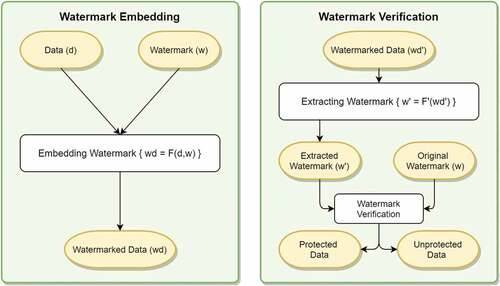
In the embedding process as shown in Figure 1, the actual watermark is embedded in the media by adding the watermark to the data. This gives the embedded data. The characteristics of the watermark are known only to the owner. During the verification phase, the watermark is extracted from the given media. If the extracted watermark matches the embedded watermark, the ownership of the media can be established. Since the media can be modified deliberately or during transmission which in turn modifies the watermark embedded, a certain error is allowed in the similarity between embedded and extracted watermarks.

Figure 1. Watermarking life cycle.

Deep Neural Network

Deep learning is a type of machine learning that uses deep neural networks (Goodfellow et al. 2016). In deep learning, the model can learn complex relations from training data without the need to manually feed the features (Shaheen et al. 2016). This is revolutionary as typical machine learning algorithms require feature extraction that is more time and resource extensive. A deep neural network consists of many stacked layers of artificial neurons. The artificial neurons are based on the functions and structures of the biological neurons. The neurons tend to fire when the activation it receives crosses a certain threshold. The artificial neural network comprises input and output layers along with the hidden layers. Each of these layers transforms the inputs given to them into some value that the next layers can use. Systems like these perform tasks by learning from various examples. The artificial units called the artificial neurons are connected in a manner that they communicate with each other similar to biological neurons to reach a particular conclusion.

Adversarial Examples

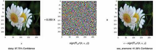
The adversarial examples as shown in Figure 2 are simply input that are designed to break the correctness of neural networks. The most common way of creating an adversarial example is to add noise to the input in such a way that the input still looks the same to the humans but causes the wrong prediction by the neural network (Goodfellow, Shlens, and Szegedy 2014).

Figure 2. Adversarial example.

Levenshtein Distance

Levenshtein distance also known as edit-distance is defined by the minimum number of one character changes required to convert one string to the other. The operations can be deletion, insertion, or substitution. It is a metric to measure the difference between two strings. E.g. Levenshtein distance for “aaa” and “aab” is one as it will take only one substitution at position 3.

MFCC

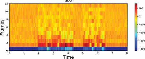
MFCC stands for Mel Frequency Cepstral Coefficients. MFCCs are a compact representation of the spectrum of an audio signal. It uses Mel scale and is commonly used in the pre-processing of audio data. Usually, 40 MFCCs are extracted per frame. But only 12–13 MFCCs are used as they contain most of the information as shown in Figure 3.

Figure 3. MFCCs of a test audio clip.

Deep Speech Model

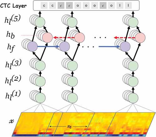
Deep Speech Model (Figure 4) is an end-to-end deep learning speech-to-text model. It is a lot simpler than the traditional speech processing systems as it does not require any pre-processing steps like feature extractionfor example, in “phoneme” based models (Gupta et al. 1995). This removed the use of any sort of dictionary like a phoneme dictionary. Deep Speech uses a dropout (Srivastava et al. 2014) rate of 5%-10% during training time. The model consists of fully connected layers, bi-directional RNN layers, a softmax layer and, a CTC layer. The architecture for Deep Speech model is shown in Figure 4

Figure 4. Deep Speech architecture.

CTC

Connectionist temporal classification (Graves et al. 2006) is a type of scoring function for training recurrent neural networks such as LSTM networks to tackle sequence problems where the length of input and output sequence is variable. The CTC algorithm assigns a probability for an output Y given an input X.

The CTC algorithm is free of alignment. It does not need to bother with an arrangement between the input and the output. CTC works by adding over the likelihood of every conceivable arrangement for the output given the input.

CTC maps the neural network outputs to string forms. It does so by introducing a special character $ϵ$. It acts as a break character. If consecutive timestamps have the same character then they will be merged. If there is an $ϵ$ between them, then they will be treated as different characters. The process is explained with an example in Figure 5

Figure 5. CTC example.

Dataset

For the generation of adversarial examples, we used the first 100 test clips of the Mozilla Common Voice dataset (Ardila et al. 2019). The dataset contains 232975 training clips, 15531 test clips, and 15531 validation clips. The audio clips are in the “MPEG Audio Layer-3” format. Since the Deep Speech model requires the “Waveform Audio File” format, the clips are converted to “Waveform Audio File” format with a sampling rate of 16000 Hz with 16-bit resolution and mono audio channel configuration.

Algorithm

We use a pre-trained Deep Speech model as our target model. Since adversarial examples are used for the proposed algorithm, there is no loss of accuracy. The algorithm is divided into two parts:

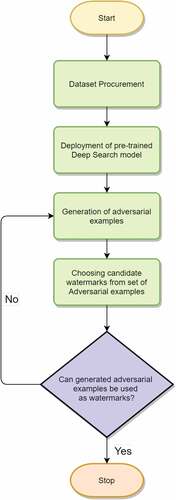
Watermark Generation

In this part, we demonstrate the watermark generation for the model. For the creation of the target string we used python “Natural Language Toolkit”(NLTK). A random phrase is generated using the text corpus provided by the NLTK library. The core part of the watermarking algorithm is the generation of the adversarial examples. We try to create an adversarial example for each audio clip in the input set. A target string is also passed along with the input audio clip. If the Levenshtein distance between adversarial example output and target phrase is zero and the amplitude is under permissible limits, we can add the example to the set to watermarks. We have found that the optimal size of the watermark set is 10 and it provides a good pay-off between confidence during watermark detection and the time taken for watermark generation. These watermarks can be used in the watermark detection algorithm to verify the ownership of the model. The process is explained as flow diagram in Figure 6.

Table

Algorithm 1 Algorithm for Watermark Generation
Input:	Original benign inputs X, Target phrase t
Output:	Set of Watermarks S
1:	procedure generate_watermarks $X,t$
2:	System Initialization
3:	$S\leftarrow \{\}$
4:	$Y\leftarrow \{\}$
5:	for each: $p\in X$ do
6:	$q\leftarrow generate\mathrm{\_}adversarial\mathrm{\_}example(p,t)$
7:	$Y\leftarrow Y\cup q$
8:	for each: $r\in Y$ do
9:	if Lev_Dis(r, t) = 0 and $dB(r)<d{B}_{max}$ then
10:	$S\leftarrow S\cup r$
11:	Return $S$

Table

Algorithm 2 Algorithm for Adversarial Example Generation
Input:	Original input x, Target phrase t, Max iterations N
Output:	Adversarial Example x
1:	procedure generate_adversarial_example $x,t$
2:	System Initialization, Adam Optimizer Initialization
3:	$u\leftarrow RandomNoise()$
4:	for $i\leftarrow 1$ to $N$ do
5:	$y\leftarrow u+x$
6:	$z\leftarrow get\mathrm{\_}logits(y)$
7:	$loss\leftarrow CTC\mathrm{\_}loss(z,t)$
8:	$y\leftarrow GradientDescent(loss,z)$
9:	if Levenshtein_Distance(Y, T) = 0 or $i=N$ then
10:	$Ad\mathrm{\_}Ex\leftarrow y$
11:	$u\leftarrow u\ast 0.8$
12:	Return $Ad\mathrm{\_}Ex$

Figure 6. Watermark generation.

Adversarial Example Generation

This algorithm creates an adversarial example for a given audio clip based on the target phrase. The main goal is to add random normal noise with a certain standard deviation to the original input and then apply gradient descent reducing the loss for the target input phrase.

First, the audio clip is pre-processed and MFCC features are calculated. Then the logits are extracted by passing the MFCC features to the Deep Speech model and capturing the output of the bi-directional RNN layers. Then the output is passed to the CTC layer to calculate the CTC loss. The loss then back-propagates to update the audio clip. If we reach the target after some iterations, we save the current modified audio as an adversarial example and prepare a new clip by adding an original audio clip to the random normal noise but with only 80% amplitude of the previously added noise. The process is then repeated to find the adversarial example with less noise. This process makes it possible to find adversarial examples with less noise. This makes the adversarial examples more suitable for the watermarking as they will sound more like the original sound. A screenshot of the expected result can be seen in Figure 7. Here, ‘path’ is the name of audio clip from the Common Voice dataset, ‘sentence’ is the transcript of the audio clip, ‘db’ is amplitude of the audio clip, ‘response’ is the output of the model after giving an adversarial example as input. ‘target’ is randomly generated target phrase, ‘lev_dis’ is the Levenshtein distance between ‘response’ and ‘target,’ ‘noise_db’ is the amplitude of the noise, ‘epochs’ are the number of epochs elapsed, ‘time’ is the time elapsed in seconds, and ‘final_db’ is the relative strength of the noise to the original audio.

Figure 7. Adversarial example generation.

Watermark Detection

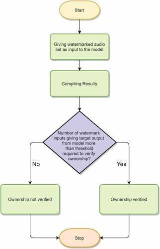
This algorithm is for the detection of watermarks and to confirm the ownership of the deep learning model. The set of watermarks generated using generate_watermarks() algorithm are used here for detection. The watermarks are passed as input to the deep learning model. If the ratio of predicted output to the target phrase is more than the threshold, the ownership of the model can be verified. The process is explained as flow diagram in Figure 8.

Figure 8. Watermark detection.

Example with Steps

1. Select target phrase: Select a target phrase that can easily verify the ownership. For example, ‘This is a property of Pulkit Rathi’ is a good target phrase.

2. Select audio input: Select audio clips that sound different from the target phrase selected in Step 1.

3. Creation of watermarks: Give the selected audio clips to watermark generation algorithm that returns ten watermarked audio clips as watermark set.

4. Watermark detection: Input the watermarked audio clips to the alleged stolen model directly or through exposed API. Capture the output returned from the model.

5. Verification of ownership: If the number of watermarked inputs that match the target phrase is more than the declared threshold, we can verify the ownership of the model. For example, if the threshold is nine and we get the target phrase i.e. ‘This is a property of Pulkit Rathi’ in our case as output from the alleged stolen model for all the ten watermarks, we can verify that the model is stolen.

Performance Metrics

Amplitude of Noise

We measure the amplitude of noise in decibels(dB). Decibel is a logarithmic scale to measure the intensity or amplitude of a sound wave. For this paper, we follow the following formula

(1) $dB(n)=ma{x}_{i}20\ast lo{g}_{10}(n_i)$(1)

Since the decibel scale is only meaningful when we have a base scale to compare with. So, we use the relative strength of noise audio to the original one.

(2) $d{B}_n(x)=dB(n)-dB(x)$(2)

where,

$d{B}_n(x)$ is noise amplitude relative to audio clip,

$dB(n)$ is amplitude of noise added,

$dB(x)$ is amplitude of audio clip.

The above equation gives negative values like “-25 dB” or “-20 dB.” This denotes that the amplitude of the noise is less than that of the original audio. The more negative this value is, the better it is suited for our use case.

Table

Algorithm 3 Algorithm for Watermark Detection
Input:	Adversarial Examples X, Target phrase t, Model m
Output:	Ownership Status
1:	procedure detect_watermark $X,t,m$
2:	System Initialization
3:	$num\leftarrow 0$
4:	for each: $u$ in $X$ do
5:	$v\leftarrow SpeechtoText(m,u)$
6:	if Levenshtein_Distance(v, t) = 0 then
7:	$num\leftarrow num+1$
8:	if num $\ge$ threshold then
9:	Ownership verified
10:	else
11:	Ownership not verified

Number of Epochs

This metric shows the number of iterations required to get the first adversarial example for an audio clip. If the optimizer converges quickly, we can get the adversarial example in less number of epochs. If we run the algorithm for more number of epochs, we get adversarial examples of relatively less noise.

(3) $d{B}_n(x)\propto 1/epoch{s}_N$(3)

where,

$d{B}_n(x)$ is noise amplitude relative to audio clip,

$epoch{s}_N$ is the number of epochs.

Time

This metric is to examine the time elapsed to get the first adversarial example for an audio clip. We can get the adversarial example in less time if the optimizer converges quickly but the amplitude of the noise will be higher.

Experiments and Results

In this section, we demonstrate various experiments, results obtained, and the conclusion derived from the results. The details of the system used for experimentation along with the list of libraries required are given in Tables 2 and 3.

Table 2. Working environment specifications

Specification	Value
RAM	12 GB
OS	64 bit Linux
Kernel version	Linux 4.19.104
GPU	12 GB Tesla K 80
CPU	64 bit Intel Xenon 2.3 GHZ

Table 3. Library version

Library Used	Version
deepspeech	0.1.1
jupyter-core	4.6.3
keras	2.3.1
nltk	3.2.5
numpy	1.18.3
pandas	1.0.3
tensorflow	1.15.2

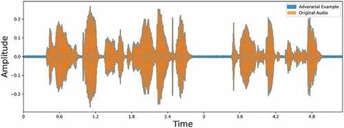
Experiment 1: Correlation between Input and Generated Adversarial Example

This experiment tells us the extent of the correlation between the input audio clip and the adversarial example generated. The adversarial example is considered a good candidate for the watermark if it is similar to the original audio.

For this experiment, we randomly choose a clip from the Common Voice test dataset. We plot the amplitude v/s time graph for the adversarial example and input the audio file. Correlation between the clips can be calculated with the correlation Equation (4)(4) $Cor{r}_{x,y}=\frac{{\sum }_{i=1}^N\left|x_i-y_i\right|}{{\sum }_{i=1}^N\left|x_i\right|}$(4) .

(4) $Cor{r}_{x,y}=\frac{{\sum }_{i=1}^N\left|x_i-y_i\right|}{{\sum }_{i=1}^N\left|x_i\right|}$(4)

The correlation between the clips turned out to be 95%. This makes the adversarial example a very good candidate for watermarking. In Figure 9, we can see that both the audio waveforms are almost overlapping. This will make it difficult for the listener to distinguish the clips but the deep learning model can differentiate the clips.

Figure 9. Overlapping audio waveform of adversarial example with 95% correlation.

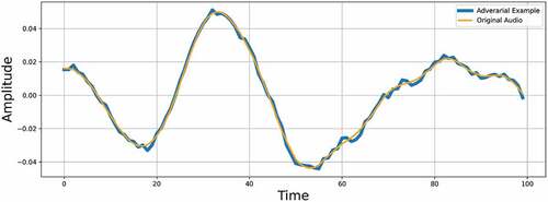
In Figure 10, we can see the waveforms of both the clips for a duration of 100 samples.

Figure 10. Waveform comparison for 100 sample points.

Experiment 2: Relation between Quality of Adversarial Example and Number of Epochs

This experiment demonstrates the relation between the number of epochs elapsed to the relative strength of noise to audio input and Levenshtein distance. We performed this experiment by generating a random two-word target phrase using the NLTK library.

(5) $Av{g}_x=\frac{{\sum }_{i=1}^N{x}_i}{N}$(5)

In Figure 11, we can see the result. The result is compiled by running the algorithm for starting 100 clips of the Common Voice test dataset and taking the average of the results obtained using Equation (5)(5) $Av{g}_x=\frac{{\sum }_{i=1}^N{x}_i}{N}$(5) .

Figure 11. Average $d{B}_n(x)$ v/s epochs.

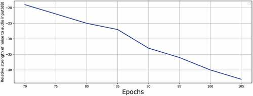
We can see that as the number of epochs increases the quality of adversarial examples also increases. The decrease in the relative strength of noise is because after the successful generation of an adversarial example, the example is saved and the algorithm tries to generate another one with the noise of lesser magnitude. This leads to a decrease in the relative strength of the noise.

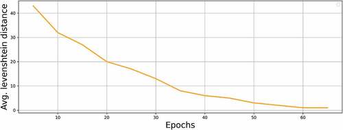
The same goes for Levenshtein distance. As the number of epochs progresses, the difference between the output of the audio clip and target string decreases as shown in Fig. 12. The more epochs algorithm runs, the more close to target output gets.

Figure 12. Average Levenshtein distance v/s epochs.

Experiment 3: Relation between Length of Target String and Number of Epochs Required

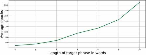
This experiment demonstrates the relation between the length of the target string with the number of minimum epochs elapsed to create an adversarial example. We performed this experiment by generating target phrases of variable length using the NLTK library.

The result is compiled by running the algorithm for all the 100 clips of the Common Voice test dataset and taking the average of the results obtained using Equation (5)(5) $Av{g}_x=\frac{{\sum }_{i=1}^N{x}_i}{N}$(5) . We can see that the time taken by the algorithm to generate the adversarial example increases with the length of the target phrase increases as shown in Figure 13. This behavior can be attributed to the fact that there are more data points in the audio to optimize and therefore the optimization algorithm is taking more time to reach the minima.

Figure 13. Average number of epochs v/s length of target phrase in words.

Experiment 4: Robustness of Watermarking Algorithm

This experiment demonstrates the robustness of the algorithm by doing three types of post-processing on the pre-trained Deep Speech model namely:

• Fine-tune last layer (FTLL) Only the last layer (fully connected layer) of the model is fine-tuned using the training data. All other layers are fixed.

• Retrain last layer (RTLL) The weights of the last layer are re-initialized and then trained with the training data. All other layers are fixed.

• Weight pruning (WP) We pruned some of the weights and then retrain the pruned model to enhance the classification accuracy. WPX stands for X% pruning of weights

We can see in Table 4 that the proposed watermark detection algorithm works with great accuracy even after doing various types of post-processing on the Deep Speech model. The experiment is done on 100 clips in the Common Voice test dataset by generating five random text sentences for each clip as target sentences. Here, accuracy is calculated as the percentage of created watermarks that are correctly identified by the watermark detection algorithm. Practically, it is not possible to reduce the accuracy of the watermarking algorithm drastically because we are not choosing audio inputs that are close to the classification boundary. We choose the input clips from all around the search space randomly and then watermark them. Even after fine-tuning the model and pruning the weights, the classification boundary moves only a bit because of the complexity of the Deep Speech model. Thus, the result of watermarked clips does not change. This makes our proposed algorithm very robust to such sort of modifications to the model. The only possible way to break the watermarking algorithm is to retrain the whole model with new data that can change the classification boundary to shift enough to break the watermarking algorithm. But this is not a practical scenario. Thus, the proposed watermark is not removable without breaking its carrier.

Table 4. Watermarking detection algorithm accuracy after post-processing model

Post-processing	Accuracy of proposed algorithm
None	100.0%
FTLL	99.5%
RTLL	98.6%
WP10	99.8%
WP20	99.7%
WP30	99.3%

Conclusion

In the present era, where the number of deep learning models is increasing day by day, it has become a necessity that a proper watermarking algorithm is used for the verification of ownership of the model. We have presented a novel watermarking algorithm to watermark the speech-to-text deep learning models using adversarial examples that can work in the black-box setting without accessing the weights of the model. The algorithm fulfills all its design goals namely fidelity, effectiveness, and robustness. The use of adversarial examples for watermarking makes it less computationally hungry and less time-consuming than other prominent watermarking algorithms for example using backdooring. The proposed watermarking approach can help to minimize the economic damage to the owner or developer of the deep learning models due to stealing and plagiarizing.

Disclosure Statement

No potential conflict of interest was reported by the author(s).

References

- Adi, Y., C. Baum, M. Cisse, B. Pinkas, and J. Keshet. 2018. Turning your weakness into a strength: Watermarking deep neural networks by backdooring. 27th {USENIX} Security Symposium Security 18, 1615–632, Baltimore, MD: USENIX Association. https://www.usenix.org/conference/usenixsecurity18/presentation/adi
- Alzantot, M., Y. Sharma, A. Elgohary, H. Bo-Jhang, M. Srivastava, and K.-W. Chang. 2018. Generating natural language adversarial examples. Proceedings of the 2018 Conference on Empirical Methods in Natural Language Processing, 2890–96, Association for Computational Linguistics, Brussels, Belgium, October-November. doi: 10.18653/v1/D18-1316.
- Ardila, R., M. Branson, K. Davis, M. Henretty, M. Kohler, J. Meyer, R. Morais, L. Saunders, F. M. Tyers, and G. Weber. 2019. Common voice: A massively-multilingual speech corpus. arXiv Preprint arXiv:1912.06670. https://lrec2020.lrec-conf.org/en/
- Carlini, N., and D. Wagner. 2018. Audio adversarial examples: Targeted attacks on speech-to-text. In 2018 IEEE Security and Privacy Workshops (SPW), San Francisco, CA, USA: IEEE, 1–7.
- Deng, J., W. Dong, R. Socher, L. Li, L. Kai, and L. Fei-Fei. 2009. Imagenet: A large-scale hierarchical image database. 2009 IEEE Conference on Computer Vision and Pattern Recognition, Miami, FL, USA, 248–55.
- Goodfellow, I. J., J. Shlens, and C. Szegedy. 2014. Explaining and harnessing adversarial examples. arXiv Preprint arXiv:1412.6572. https://arxiv.org/abs/1412.6572
- Goodfellow, I., Y. Bengio, A. Courville, and Y. Bengio. 2016. Deep learning, vol. 1. Cambridge: MIT press.
- Graves, A., S. Fernández, F. Gomez, and J. Schmidhuber. 2006. Connectionist temporal classification: Labelling unsegmented sequence data with recurrent neural networks. ICML '06: Proceedings of the 23rd International Conference on Machine Learning, Pittsburgh, Pennsylvania, USA: Association for Computing Machinery, 369–76. doi: 10.1145/1143844
- Gupta, V. N., M. Lennig, P. J. Kenny, and C. K. Toulson. Phoneme based speech recognition, February 14 1995. US Patent 5,390,278.
- Han, S., J. Pool, J. Tran, and W. Dally. 2015. Learning both weights and connections for efficient neural network. In Advances in neural information processing systems, ed. C. Cortes and N. Lawrence and D. Lee and M. Sugiyama and R. Garnett, 1135–43. Montreal, Quebec, Canada: MIT Press.
- He, K., X. Zhang, S. Ren, and J. Sun. 2016. Deep residual learning for image recognition. Proceedings of the IEEE conference on computer vision and pattern recognition, Las Vegas, Nevada, USA, 770–78.
- Namba, R., and J. Sakuma. 2019. Robust watermarking of neural network with exponential weighting. CoRR, abs/1901.06151. http://arxiv.org/abs/1901.06151.
- Shaheen, F., B. Verma, and M. Asafuddoula. 2016. Impact of automatic feature extraction in deep learning architecture. 2016 International conference on digital image computing: techniques and applications (DICTA), 1–8. IEEE, Gold Coast, QLD, Australia.
- Srivastava, N., G. Hinton, A. Krizhevsky, I. Sutskever, and R. Salakhutdinov. 2014. Dropout: A simple way to prevent neural networks from overfitting. The Journal of Machine Learning Research 150 (1):1929–58.
- Szegedy, C., W. Zaremba, I. Sutskever, J. Bruna, D. Erhan, I. Goodfellow, and R. Fergus. 2013. Intriguing properties of neural networks. arXiv Preprint arXiv:1312.6199. https://arxiv.org/abs/1312.6199
- Uchida, Y., Y. Nagai, S. Sakazawa, and S. Shin’ichi. 2017. Embedding watermarks into deep neural networks. In Proceedings of the 2017 ACM on International Conference on Multimedia Retrieval, ICMR ’17, 269–77, Association for Computing Machinery, New York, NY, USA. doi: 10.1145/3078971.3078974.
- Zhang, J., G. Zhongshu, J. Jang, W. Hui, M. P. Stoecklin, H. Huang, and I. Molloy. 2018. Protecting intellectual property of deep neural networks with watermarking. Proceedings of the 2018 on Asia Conference on Computer and Communications Security, ASIACCS ’18, 159–72, Association for Computing Machinery, New York, NY, USA. doi: 10.1145/3196494.3196550.