A Cluster Analysis Methodology for the Categorization of Soil Samples for Forensic Sciences Based on Elemental Fingerprint

ABSTRACT

Soil and dirt fragments are easily transferred from the ground to objects such as clothing, shoes, skin, nails, and tires. The elemental analysis of these samples involved in crimes can be an important source of information for forensic scientists because they can present substantial evidence by creating links between victims, suspects, crime scenes and other relevant actors or places. In this work we present a promising new approach for the study of soil samples, using data mining techniques applied to the elemental fingerprints of soil. We experimented on soil samples obtained from southeast Oregon and northern Nevada, two neighboring states in the United States that have similar geological characteristics while also displaying some specific differences. The chemical composition of soil and sediments samples were determined by the use of inductively coupled plasma-mass spectrometry (ICP-MS). Thirty-three elements were analyzed, and we used their concentrations to conduct the analysis. Cluster analysis was performed employing the K-means clustering algorithm. We found three clusters that showed interesting chemical patterns. In order to investigate the most significant chemical elements that distinguish the clusters, we employed the Correlation-Based Feature Selection (CFS) algorithm. Lastly, we developed a classification model based on support vector machine (SVM), which can predict in which of the found clusters an arbitrary soil sample would fall with a 99% prediction accuracy when all 32 variables were used for training the model, and a 95% prediction accuracy when only the 10 most relevant elements were used for training the model. Following this methodology, forensic scientists and experts would be able to establish profiles of soil samples extracted from the crime scene and nearby regions, and use classification models to predict which of these profiles an arbitrary soil sample found on the subjects involved in the crime would be associated with.

Introduction

The investigation of soil is a relatively new approach in forensic sciences, one that has aided in solving a number of crimes. For instance, the analysis of elemental fingerprints of soil samples extracted from a crime scene, the suspect’s car and areas nearby or far away, helped solve a murder case that occurred in Italy (Concheri et al. 2011). Lorna Dawson, head of soil forensics at the James Hutton Institute in Scotland, was a pioneer in bringing chromatography, mass spectrometry and other advanced soil science techniques into forensic sciences, and developing powerful new approaches (Wald 2015).

The motivation for the analysis of soil in forensic sciences lies in the complexity of soil composition, which can widely vary depending on local characteristics such as climate, topography, pollution, age, human activities and other factors, thereby yielding specific yet different elemental fingerprints for soil in different sites (Wu et al. 2018). Because soil and dirt fragments are easily transferred from the ground to objects such as clothing, shoes, skin, finger nails, and tires, they can lead to potential links between victims, suspects, crime scenes and other relevant actors or places (Reidy et al. 2013). In addition to forensic sciences, the study of geochemical data and elemental fingerprinting of soil and sediments has provided meaningful information for various applications such as earth and ocean science, archeology, human health and other fields (Owens et al. 2016).

One promising manner of extracting information from geochemical data is the approach of using data mining, which is a knowledge discovery process that utilizes powerful techniques that combine mathematic optimization, machine learning and statistics for uncovering hidden patterns and information in raw data. Data mining processes involve data classification, cluster analysis, feature selection and other methods. Recent studies report the use of data mining techniques for the profiling of fine-grained soils regarding shear strength and the plasticity index (Goktepe, Altun, and Sezer 2005), prediction of organic matter and clay (Teixeira et al. 2014), classification of soil textures based on terrain parameters (Wu et al. 2018), and others. Regarding forensic discrimination of soil samples, the use of chemometrics is widely reported in the literature, with successful application of techniques such as PCA (Dragović and Onjia 2006; Melo et al. 2008; Xu et al. 2020), PCA combined with discriminant analysis (Chauhan et al. 2021; Reidy et al. 2013; Thanasoulias et al. 2002), linear and partial least squares discriminant analysis (Baron et al. 2011), factor analysis (Mazzetto, Dieckow, and Bonfleur 2018), PCA and ANOVA (Martin et al. 2021), k-means (Hu et al. 2020), and so on. To our knowledge, this is the first study to use advanced data mining techniques such as feature selection and support vector machines.

In this study we present a new methodology for the categorization and prediction of soil samples by using data mining techniques – namely cluster analysis along with feature selection and classification algorithms, which was applied to the chemical composition of soil samples. Our goal was to identify natural groups existing within the analyzed soil samples and provide classification models that can predict to which of these groups an arbitrary soil sample would belong. Following this methodology, forensic scientists and experts can establish characterizations of soil samples extracted from crime scenes and areas near to crimes, and use classification models to predict in which of these characteristics an arbitrary soil sample found on the subjects involved in the crime would fall. Since we analyzed the chemical composition of soil samples, we expected that samples gathered near one another from specific sites would have similar elemental fingerprints, and therefore, the profiles established by the clustering algorithms would basically be formed by soil samples taken from nearby sites. In order to confirm this assumption, we worked with soil samples obtained from two neighboring US states, Oregon and Nevada. Despite the location of studied soil samples, our methodology can be applied to any other location.

The landscape in southeastern Oregon is characterized as a barren desert, the central region is distinguished by volcanic rock formations with lava beds. In northern Nevada, the Humboldt River crosses what is characterized as a mild desert. For the most part, both regions are situated inside contiguous endorheic watersheds known as the Great Basin, with an arid climate. Hence, we expected to see some level of dissimilarity in the elemental fingerprint of the soil samples from the two regions. We also applied a feature selection technique that allowed us to determine the most relevant chemical elements for the differentiation of soil profiles.

The main contributions of this paper are:

• We introduced a new methodology for the analysis of soil sample data to aid forensic sciences. The use of cluster analysis combined with elemental fingerprint data for analysis of soil samples is new in the literature and can be a useful source of information for forensic sciences.

• We determined soil characterization taken from southeast Oregon and northern Nevada with the application of clustering algorithms, and develop classification models capable of predicting which of these profiles a new, unknown soil sample would be associated with.

• We employed a feature selection algorithm to find the most relevant chemical elements for the discrimination of the formed profiles of soil.

Materials and Methods

The Northern Great Basin Geochemical Dataset

We worked with the northern Great Basin geochemical dataset provided in United States Geological Survey (USGS) open-file report 02–227 (Coombs et al. 2002). The USGS is a science agency that constantly provides various data and studies about natural resources, ecosystems, the environment, climate, land-use changes, natural hazards, geological structures and other information about the Earth. Publications are written by USGS scientists and are gathered in the USGS Pubs Warehouse, and the analyzed datasets are published for free downloading, along with print publications.

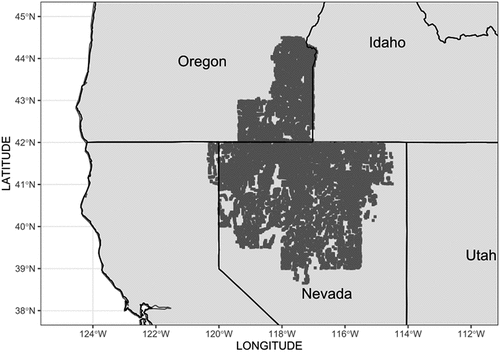
The geochemical dataset presented in the report is a compilation of the chemical composition of 10,261 stream-sediment and soil samples collected during the National Uranium Resource Evaluation’s (NURE) Hydrogeochemical and Stream Sediment Reconnaissance (HSSR) program of the Department of Energy. Samples were collected from 1977 to 1983 in southeastern Oregon, southwestern Idaho, northeastern California, and northern Nevada. The dataset was reanalyzed to support a series of mineral-resource assessments by the USGS, which also included additional samples taken in 1992. The study area is illustrated in Figure 1.

Figure 1. Location of the study area and collected samples.

The laboratories that participated in data sample collection and analysis included the Savannah River Laboratory (SRL), the USGS, the Lawrence Livermore National Laboratory (LLL) and the Bendix Field Engineering Corp (under LLL). The samples were collected and processed using a variety of protocols, and the quality of the data was evaluated using concurrent analysis of the samples and standard reference material (SRM) by two geochemical methods: “ICP-40,” which consists of having the samples dissolved in a series of acids (hydrochloric, nitric, perchloric, and hydrofluoric acids (Briggs 1996)), with the resultant solution being analyzed through inductively coupled plasma atomic emission spectrometry (ICP-AES), an approach that allows 40 elements to be analyzed simultaneously at detection limits, plus “ICP-Partial,” which partially dissolves the samples in weaker acids and an organic extraction, allowing for the simultaneous determination of 10 to 15 elements.

In addition to the concentrations of the chemical elements determined in the soil and sediment samples, the dataset also provides for each sample the following metadata: a unique identifier, a number assigned by the collection laboratory, the sample type (an indicator of the sample source, medium or treatment), the mineral-resource study under which the sample was analyzed, the quadrangle from which the sample was collected, and the longitude and latitude in decimal degrees of the sample site.

Since our goal is to uncover natural groupings of soil samples based solely on their chemical composition, we ignored these metadata in order to prevent them from biasing the results. We also discarded measurements produced by the ICP-Partial method and kept only the measurements produced by the ICP-40 method in order to reduce redundancy. A complete description of the original dataset can be found in the open report’s official website (https://pubs.usgs.gov/of/2002/0227/intro.html). The variables analyzed in this work, after reducing the original dataset, are summarized in Table 1. Although the variables longitude and latitude were also excluded from the statistical and data mining analysis, we retained them in the dataset, as they allow us to trace the location from which samples were collected. The rest of the analyzed variables refer to the concentrations of the elements identified in the samples using the ICP-40 method. The majority of these elements were reported as parts per million, except for Al, Ca, Fe, K, Mg, Na, P and Ti, all of which were reported as weight percentage.

Table 1. Descriptive variables of the northern Great Basin geochemical data set that were considered for analysis in this work

Variable	Description	Variable	Description
LONGITUDE	Longitude, in decimal degrees, of the sample site. Negative numbers indicate west longitudes. These values are assumed to be based upon the NAD27 Datum and Clarke 1866 Ellipsoid.	Li	Elemental concentration of lithium in parts per million.
LATITUDE	Latitude, in decimal degrees, of the sample site. Positive numbers indicate northern latitudes. These values are assumed to be based upon the NAD27 Datum and Clarke 1866 Ellipsoid.	Mg	Elemental concentration of magnesium in weight percent.
Ag	Elemental concentration of silver in parts per million.	Mn	Elemental concentration of manganese in parts per million.
Al	Elemental concentration of aluminum in weight percent.	Mo	Elemental concentration of molybdenum in parts per million.
As	Elemental concentration of arsenic in parts per million.	Na	Elemental concentration of sodium in weight percent.
Ba	Elemental concentration of barium in parts per million.	Nb	Elemental concentration of niobium in parts per million.
Be	Elemental concentration of beryllium in parts per million.	Ni	Elemental concentration of nickel in parts per million.
Ca	Elemental concentration of calcium in weight percent.	P	Elemental concentration of phosphorus in weight percent.
Cd	Elemental concentration of cadmium in parts per million.	Pb	Elemental concentration of lead in parts per million.
Ce	Elemental concentration of cerium in parts per million.	Sc	Elemental concentration of scandium in parts per million.
Co	Elemental concentration of cobalt in parts per million.	Sn	Elemental concentration of tin in parts per million.
Cr	Elemental concentration of chromium in parts per million.	Sr	Elemental concentration of strontium in parts per million.
Cu	Elemental concentration of copper in parts per million.	Th	Elemental concentration of thorium in parts per million.
Fe	Elemental concentration of iron in percent.	Ti	Elemental concentration of titanium in percent.
Ga	Elemental concentration of gallium in parts per million.	V	Elemental concentration of vanadium in parts per million.
K	Elemental concentration of potassium in percent.	Y	Elemental concentration of yttrium in parts per million.
La	Elemental concentration of lanthanum in parts per million.	Zn	Elemental concentration of zinc in parts per million.

Cluster Analysis

Cluster analysis is a branch of exploratory analysis and refers to the identification and study of natural groups, or clusters, that exist within a data set. According to (Jain 2010), data clustering can be defined as the process of finding K groups in a representation of n objects, based on a measure of similarity such that the similarities among objects in the same group are high, while the similarities among objects in different groups are low. Clustering algorithms implement unsupervised learning, since the process of determining clusters does not count with any previously labeled data, and are useful for various purposes such as the discovery of hidden patterns within the data, data compression, determining the degree of similarity (or dissimilarity) between two objects, and so on. Cluster analysis has had applications in various fields such as forensic sciences (Maione et al. 2018), swarm intelligence (Dhote, Thakare, and Chaudhari 2013), glutamic acid fermentation (Wang, Xu, and Jiang 2016), cosmology (Beutler et al. 2014), financial risk analysis (Kou, Peng, and Wang 2014), image retrieval (Rahmani, Pal, and Arora 2014), healthcare (Elbattah and Molloy 2017; Lee 2015).

One of the most popular algorithms for data clustering is the K-means. This is due to its simplicity, ease of implementation, efficiency and empirical success, as noted in the cluster analysis literature (Jain 2010). K-means identifies k clusters, which are represented by the mean value of all points within the clusters, known as centroids. The clusters are determined by K-means according to the following steps:

1. Randomly choose k instances of the data set and identify them as centroids;

2. For all instances x in the data set: determine the centroid that is nearest to x, and assign x to the same cluster of this particular centroid.

3. Update all centroids to establish the mean value, or center of mass, of the instances in their respective clusters.

4. Repeat steps 2 and 3 until no changes can be made to the centroids.

In this work, we use the Hartigan-Wong algorithm implementation for K-means (Hartigan and Wong 1979), and the Euclidean distance to compute the distance between the instances and the centroids.

K-means-based clustering algorithms mainly require the number of clusters to be formed from the data as an input parameter. One of the main issues in cluster analysis on real data sets is finding an appropriate number of clusters within the data, since pure clustering problems in exploratory analyses do not count regarding labeled data and rarely have any information beforehand regarding natural groups that exist within the data.

There are several techniques in the present literature that can aid in estimating this number. The NbClust package (Charrad et al. 2014) that is available for the R software (R Core Team 2020) offers a function that can estimate the best number of clusters within a data set, according to 30 distinct indexes, including silhouettes, gap statistics, biserial correlation, gamma statistics and other measures. A range of values in which the number of clusters will be searched must be specified beforehand, and the best number of clusters is computed as the number within a range that was most voted by these various indexes.

Data Classification with Support Vector Machines

Data classification is the core step for predictive analyses and refers to the process of predicting labels for unknown samples based on the content of their descriptive features. Data classification is performed by using classification models which have been developed through supervised learning. This means that a set of labeled samples is used to train the models before they are ready to predict new ones. Therefore, classification models use the knowledge acquired from data previously observed to predict the class label of new samples. Conceptually, classification models are defined as decision functions capable of mapping a set of variables into a class label (Tan, Steinbach, and Kumar 2005). While clustering algorithms divide a set of unlabeled data samples into distinct clusters based on hidden patterns of similarity (or dissimilarity), classification models are useful for stating with which of the found clusters a new arbitrary sample would be associated.

Data classification has been widely applied in various fields and for numerous purposes, such as recognition of geographical origin of food and drink (Ceballos-Magaña et al. 2012; da Costa, Castro, and Barbosa 2016), authenticity of organic food(Barbosa et al. 2015; Maione et al. 2016a, 2016b), forensic science (Maione et al. 2018), sentiment analysis (Griol and Molina 2015), diagnosis (Krishnaiah, Narsimha, and Chandra 2013; Sumbaly, Vishnusri, and Jeyalatha 2014) and survivability (Delen, Walker, and Kadam 2005) of cancers patients, prediction of final fruit weights in horticulture (Rad, Fanaei, and Rad 2015).

One of the most known classification models in the recent data classification literature, due to its efficiency and empirical success, is the use of support vector machines (SVM). SVM is a binary classification model proposed by (Cortes and Vapnik 1995) that can successfully be extended to multiclass problems by using the one-versus-all approach: a model is developed for each pair of available class labels, and the class predicted by the most classifiers is chosen as the class label for an arbitrary sample. SVM searches for the decision boundary, also called hyperplane, with the largest margin possible.

For C-SVM classification, a parameter C is introduced in the optimization problem in order to penalize prediction errors and minimize the overall training error (Abidine and Fergani 2012). The greater the parameter C, the harder the optimization will be, and a lower parameter C will emphasis a wider overall separation hyperplane (Lantz 2013). Moreover, kernel functions aid SVM in finding linear decision boundaries by transforming and projecting data samples into new feature spaces, which is often called “the kernel trick.” The radial basis function kernel (RBF) function, which we employ in this work, requires a smoothing parameter γ (gamma). Both parameters C and γ can be tuned in order to provide SVM models with superior classification performance. In this work we performed a grid search on the values $\mathrm{C}=\left\{0.25,0.5,1,1.5,2,10,100\right\}$ and $\gamma =\left\{1,0.5,0.1,0.01,0.02,0.03\right\}$ for each model developed and selected the pair of parameters (C,$\gamma$) as observed on the model having the best prediction accuracy.

Estimating the prediction accuracy of a classification model requires testing the model after its training phase. A common practice is to divide the data set into two exclusive subsets, one for training the model, the other for testing it. The final is computed by dividing the number of correct classifications by the number of total samples in the test set.

The main issue with this approach lies in the randomness with which the samples fall, either on the training or test set. Training the model with different samples will likely change the final prediction accuracy of the model, especially if the proportion of classes in training and tests is imbalanced (Kohavi 1995). Cross validation is a useful method for achieving a more stable level of accuracy. In k-fold cross validation, the data set is divided into k mutually exclusive partitions. For each iteration, one partition will pose as the test set, while the others will train the model. This process is repeated k times, until all single partitions are used to test the model. In this study, we used $\mathrm{k}=10$ folds.

Feature Evaluation

Both the quality of the final clusters obtained by using a clustering algorithm and the prediction accuracy of classification models are highly influenced by the feature variables of the data set. Feature selection methods evaluate the significance of the features and the subset of features, and identify those that are more relevant for the classification process. Regarding our project, we set out to investigate which chemical components have more influence on the decision of the classification model, to determine into which cluster an arbitrary soil sample would fall. We also aimed to find a subset with a smaller number of descriptive features, one that could still yield a classification model with good prediction accuracy for predicting the cluster for new soil samples.

The Correlation-based Feature Selection (CFS) method (Hall 2000) divides the original feature set into different subsets consisting of combinations of features. Each subset is measured in terms of the correlation between its features and the class label, and the inter-correlation between these features. A well-rated feature subset is expected to be composed of features that present little dependence on one another and, at the same time, a high degree of dependence from the class label. The CFS algorithm uses the Pearson correlation to compute feature correlations. The merit of each subset is provided by the equation:

(7) $M\left(S\right)=\frac{m\overline{r_{cf}}}{\sqrt{m+m\left(m-1\right)\overline{r_{ff}}}}$(7)

in which m is the number of total features which describe the data set, $\overline{r_{cf}}$ is the average correlation between the features in subset S and the class label, and $\overline{r_{ff}}$ is the average intercorrelation between the features in subset S (Hall 2000).

We also computed the Pearson correlation for each feature and the class label in order to check which chemical elements has had more of an effect on the clusters.

Results and Discussion

The chemical components found in the analyzed soil and sediments samples and their mean concentrations, along with standard deviation values, are presented in Table 2. The most present elements in the studied data samples are barium, manganese and strontium, with mean concentration values of approximately 915, 886 and 361 ppm, respectively. The chemical elements found in the samples are very similar to those determined by (Melo et al. 2008) and by (Reidy et al. 2013), with some expected differences.

Table 2. Statistical measures (mean and standard deviation) for the concentrations of chemical components found in soil samples

Element	Mean ± Standard Deviation (ppm)	Element	Mean ± Standard Deviation (ppm)	Element	Mean ± Standard Deviation (ppm)
Ag	1.06 ± 2.10	Fe	3.63 ± 1.75	P	0.08 ± 0.04
Al	7.43 ± 1.13	Ga	17.8 ± 3.35	Pb	23.0 ± 273
As	11.6 ± 33.0	K	2.01 ± 0.54	Sc	10.4 ± 5.38
Ba	914.9 ± 469.8	La	36.5 ± 17.7	Sn	2.29 ± 6.15
Be	1.68 ± 0.87	Li	29.6 ± 20.9	Sr	363.1 ± 179.1
Ca	2.81 ± 2.12	Mg	1.00 ± 0.64	Th	10.2 ± 7.94
Cd	1.09 ± 1.51	Mn	886.3 ± 427.2	Ti	0.50 ± 0.29
Ce	67.7 ± 30.8	Mo	2.31 ± 2.78	V	114.4 ± 82.7
Co	14.5 ± 9.25	Na	1.80 ± 0.62	Y	23.8 ± 9.08
Cr	92.6 ± 94.0	Nb	14.18 ± 5.72	Zn	95.8 ± 195
Cu	31.1 ± 55.0	Ni	24.5 ± 33.9

All the elements determined in Brazilian soil samples, as investigated by (Melo et al. 2008), that expected to find sulfur, antimony and silicon, were also found in our samples. The number of elements determined in their soil samples was also somewhat smaller (19 elements). (Reidy et al. 2013) also found fewer chemical elements in their soil samples, as collected in Mississippi, USA. This state is situated approximately 1800 miles to the east from the northern Great Basin area where our analyzed samples were collected. From the 22 elements determined in their soil samples, only cesium, rubidium, selenium and uranium are absent in our analyzed samples. Finally, both studies and our dataset report the presence of Al, As, Ba, Ca, Cr, Cu, Fe, K, Mg, Mn, Ni, Pb and Zn in soil and sediment samples.

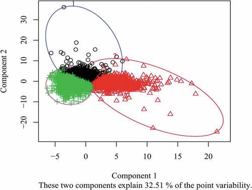
For the data analysis, our first step was to estimate an appropriate number of clusters to be found within the data. The thirty indexes implemented in the NbClust package for R software were consulted, and the most voted number of clusters was 3. The K-means clustering algorithm was applied, and 4713 samples were associated with Cluster 1, 1693 samples were associated with Cluster 2, and 3853 samples were associated with Cluster 3. The distribution of the samples in each of the three clusters can be seen in Figure 2, expressed by the two principal components that were extracted through principal component analysis (PCA) in order to ease visualization. Some overlap can be observed in data points associated to Cluster 1 (black circles) and 2 (red triangles), which was expected, since some concentration values presented high variability for various chemical elements found in the samples, as can be seen in Table 2.

Figure 2. Distribution of samples in the three clusters, divided by the K-means expressed by the two principal components. Cluster 1 = black circles, Cluster 2 = red triangles and Cluster 3 = green crosses.

The statistical measurements of the concentration values for each individual cluster of soil samples are shown in Table 3, along with standard deviations. We can notice that, especially in samples associated with Cluster 2, the mean concentrations values for Ag, As, Cd, Cu, Ni, Pb and Sn are fairly smaller than their own standard deviations. Except for As, whose determined levels are highly sparse in the three clusters, these elements are more stable (less variable) in samples from Cluster 1 (except for tin) and Cluster 3 (except for silver and lead).

Table 3. Mean and standard deviation values for the concentrations of the chemical elements in soil samples taken from the three clusters

Element	Cluster 1 Mean ± SD (per above)	Cluster 2 Mean ± SD (per above)	Cluster 3 Mean ± SD (per above)
Ag	1.02 ± 0.88	1.16 ± 4.27	1.08 ± 1.68
Al	7.78 ± 0.65	8.36 ± 1.02	6.60 ± 1.10
As	8.61 ± 15.0	11.2 ± 58.1	15.5 ± 33.3
Ba	834.5 ± 302.8	760.7 ± 351.8	1081.4 ± 613.1
Be	2.05 ± 0.93	1.42 ± 0.60	1.33 ± 0.70
Ca	2.29 ± 1.02	3.60 ± 1.49	3.01 ± 2.99
Cd	1.01 ± 0.17	1.21 ± 3.56	1.14 ± 0.67
Ce	72.7 ± 36.3	57.4 ± 22.5	66.1 ± 24.8
Co	13.9 ± 4.72	28.7 ± 12.4	9.03 ± 3.81
Cr	49.5 ± 35.8	102.2 ± 69.1	141 ± 123.3
Cu	25.9 ± 12.6	59.9 ± 125.8	24.7 ± 21.4
Fe	3.45 ± 0.94	6.22 ± 2.48	2.70 ± 0.72
Ga	19.1 ± 2.15	20.7 ± 3.23	15.0 ± 2.43
K	2.10 ± 0.50	1.38 ± 0.39	2.17 ± 0.46
La	38.0 ± 20.6	27.4 ± 12.1	38.8 ± 14.4
Li	31.4 ± 24.1	22.0 ± 9.12	30.6 ± 19.8
Mg	0.83 ± 0.33	1.60 ± 0.78	0.96 ± 0.72
Mn	900.2 ± 338.8	1288.7 ± 615.4	692.2 ± 264.8
Mo	1.28 ± 1.07	1.22 ± 1.49	4.05 ± 3.65
Na	2.02 ± 0.54	2.08 ± 0.52	1.41 ± 0.54
Nb	16.9 ± 5.69	15.4 ± 4.82	10.2 ± 3.40
Ni	18.7 ± 9.33	46.1 ± 76.0	21.9 ± 13.1
P	0.07 ± 0.03	0.12 ± 0.05	0.08 ± 0.04
Pb	18.9 ± 9.45	29.9 ± 668	25.1 ± 46.9
Sc	10.5 ± 3.03	19.1 ± 5.51	6.50 ± 2.02
Sn	2.23 ± 2.52	2.51 ± 14.4	2.27 ± 1.24
Sr	357.1 ± 134.4	452.2 ± 159.1	331.2 ± 218.3
Th	10.8 ± 9.59	6.20 ± 6.37	11.30 ± 5.35
Ti	0.50 ± 0.20	0.90 ± 0.40	0.32 ± 0.10
V	95.7 ± 36.4	232.3 ± 131.2	85.4 ± 40.7
Y	27.1 ± 10.5	24.5 ± 6.57	19.4 ± 5.75
Zn	86.4 ± 33.5	126.9 ± 461.8	93.5 ± 75.2

Cluster 1: Soil samples in Cluster 1 present inferior mean concentration values for As, Cr, Ni and Zn compared to the samples from other clusters, but higher mean levels of Ce. Levels of As and Cr are particularly lower in comparison to samples in Cluster 3, and Ni and Zn in comparison to Cluster 2.

Cluster 2: Samples from Cluster 2 show higher mean levels of Al, Co, Cu, Fe, Mn, Ni, Sc, Sr, V and Zn than samples from others clusters, but inferior mean values of Ba and Th, especially in comparison to samples from Cluster 3. Levels of Cu, Ni, Sr, V and Zn are higher for samples in this Cluster, while samples in Cluster 1 and 3 present a similar lower mean concentration for these elements.

Cluster 3: Mean concentration levels of As, Ba, Cr, Mo and Th are higher in samples from Cluster 3 than from other clusters, but inferior for Co, Fe, Mn, Sc and V. While the other two clusters have a similar mean concentration for Mo, samples in Cluster 3 present a higher mean concentration for this element. Samples from Cluster 2 present approximately double of the mean concentration of Mn and Ni in relation to samples in Cluster 3, and three times the mean concentration of Co, Sc, V and Fe. On the other hand, samples in this cluster present almost three times the mean concentration of Cr than samples in Cluster 1.

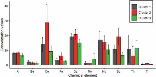
Considering the cluster values (1, 2 or 3) as the class label for the samples, the CFS method resulted in the chemicals Al, Be, Co, Fe, Ga, Mo, Nb, Sc, Th and Ti as the subset of chemical elements that is most relevant to discriminate the samples from the three clusters. The mean concentration values of these elements alone in each cluster are shown in Figure 3. An immediate visible pattern is that samples in Cluster 2 present considerably higher mean values of Co, Fe and Sc than samples in other clusters. Moreover, samples in Cluster 3 show lower mean values for all ten elements compared to the other clusters, except for Mo and Th. Samples from Cluster 1 show higher mean values for Be and Nb when compared to the other clusters.

Figure 3. Mean values for the concentration of the ten most relevant elements determined by the CFS feature selection technique.

These associations reveal that the ten chemical elements are more correlated to distinguish Cluster 1, Cluster 2, and Cluster 3 using their values. In Figure 4, we plot the location of the extraction of the soil samples. On the map, samples are colored according to their respective cluster, whereas Cluster 1 consists of black dots, Cluster 2 red dots, and Cluster 3 green dots. Interestingly, almost no samples from Cluster 3 occur in Oregon, and most of the samples collected in this state are associated with Cluster 1. Samples from Cluster 3 are basically concentrated in the eastern region of Nevada, along with samples from Cluster 1, and almost no samples from Cluster 2 are observed in this region. Samples from the latter are scattered throughout Oregon and the western region of Nevada, mingled with samples from Cluster 1.

Figure 4. Map from the location from which each sample was collected. Cluster 1 = gray, Cluster 2 = red and Cluster 3 = green.

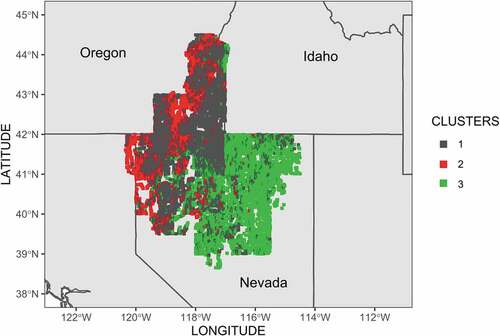
This visualization of the clusters on the map results in some interesting observations for the forensic sciences. For example, consider that a corpse was found in the southeastern region of Nevada, as shown on the map in Figure 4. As stated, this region is visibly dominated by samples from Cluster 1 (red dots), and almost no samples associated with Cluster 3 occur in this region. The elemental fingerprint of any soil samples found under the body’s fingernails, soles of shoes, clothes or elsewhere could be input into a classification model, which would predict which of the three clusters these samples would be associated with, according to the chemical composition pattern. In this particular case, the expected result should be found in Cluster 1; otherwise, the corpse was likely moved to this place after the murder. Likewise, a corpse found in southeastern Oregon is expected to carry no soil samples associated with Cluster 3. On another scenario, soil samples found in the sole of the shoes of a crime suspect could reveal where he or she possibly walked at the time of the crime.

Of course, the scenarios described above depend upon classification models with high prediction accuracies in order to reach fruition. The idea is to build reliable models capable of predicting which cluster an arbitrary and unknown soil sample collected from victims and/or suspects would be associated with, based on its chemical composition. Pursuing this idea, we developed classification models based on SVM for two cases: in the first, all chemical elements found in the soil samples were considered to be features for training; in the second case, only the most relevant subset of features, composed by the ten elements identified by the CFS, was considered for training. In addition to comparing the results and employing the model with the best degree of accuracy, we also wanted to investigate the possibility of achieving a classification model based on fewer elements, but still with good predictive results.

The Accuracy values achieved by the two C-SVM models are shown in Table 4. The model that focused on all 33 chemical elements from the original feature set performed better, presenting an approximately 99% prediction accuracy. The best values computed for C and γ parameters through grid search were 100 and 0.01, respectively. However, the C-SVM model trained on the 11 chemical elements determined by the CFS as the most relevant feature subset achieved approximately a 95% prediction accuracy, which still is an excellent measure and was obtained from only one-third of the variables. Therefore, we achieved classification models capable of predicting, with high performance, into which of the three found clusters an arbitrary soil sample would fall.

Table 4. Accuracy values achieved by the SVM models developed on the original feature set and on the feature subset determined by the CFS. The best values for the model parameters computed by grid search are also shown

Model info	Original feature set (32 chemical elements)	CFS feature subset (10 chemical elements)
Accuracy	99.03%	95.37%
C parameter value	100	2
γ parameter value	0.01	0.1

In this way, we proved that the provided methodology, which combined cluster analysis with K-means – classification models based on SVM and CFS techniques for feature selection – can be used as a promising source of information for forensic sciences.

Conclusion

In this work we presented a new methodology for the analysis of soil samples to aid forensic sciences. Our proposed methodology combines data mining techniques and elemental fingerprinting of soil, and was performed in three steps.

The first step set out to conduct a cluster analysis in order to determine characteristics for the soil samples analyzed. In this study, we experimented on soil samples obtained from southeastern Oregon and northern Nevada. Since the geology in both regions shows similar characteristics due to the proximity of these two states, while showing some specific differences, we nevertheless expected a feasible level of dissimilarity in the elemental fingerprint of the soil samples from these two regions. The best number of clusters, three, was estimated by the indexes available in the NbClust package of R software. We applied the K-means clustering algorithm. The majority of soil samples collected in southeastern Oregon and the western part of northern Nevada are associated with the same cluster, named Cluster 1, albeit with samples from Cluster 2 spread among them. The soil samples obtained in central Nevada and in the eastern part of northern Nevada are associated with the third cluster, named Cluster 3, with a few samples from Cluster 1 also observed in these areas – possibly as outliers. Almost no samples from Cluster 3 occurred in Oregon, nor did samples from Cluster 2 occur in the eastern part of Nevada; the few samples from these particular clusters observed in these regions can possibly be outliers.

Chemical patterns were also observed in the three clusters. In short, soil samples in Cluster 1 presented less concentration values for As, Cr, Ni and Zn than those of other clusters, but higher mean levels of Ce. Samples from Cluster 2 showed higher levels of Co, Cu, Fe, Mn, Ni, Sc, Sr, V and Zn compared to samples from others clusters, but inferior mean values of Ba and Th. Samples from Cluster 3 showed higher levels of As, Ba, Cr, Mo and Th, but inferior levels of Co, Fe, Mn, Sc and V.

The second step involved determining the most relevant chemical elements for the differentiation of the clusters. We applied the CFS technique, which selected 10 of the 32 original chemical components as the most significant. The selected elements were Al, Be, Co, Fe, Ga, Mo, Nb, Sc, Th and Ti.

The third and final step entailed performing data classification with classification models based on C-SVM, which could predict into which cluster an unknown soil sample would fall. When all available chemical components were used for training, the model reached a 99% prediction accuracy. When only the eleven most significant elements determined by the CFS were used for training, the model reached a 95% prediction accuracy, which is still a very high level of performance.

Disclosure Statement

No potential conflict of interest was reported by the author(s).

References

- Abidine, M. B., and B. Fergani. 2012. Evaluating C-SVM, CRF and LDA classification for daily activity recognition. In 2012 International Conference on Multimedia Computing and Systems, 272–844. doi:10.1109/ICMCS.2012.6320300.
- Barbosa, R. M., B. L. Batista, C. V. Barião, R. M. Varrique, V. A. Coelho, A. D. Campiglia, and F. Barbosa. 2015. A simple and practical control of the authenticity of organic sugarcane samples based on the use of machine-learning algorithms and trace elements determination by inductively coupled plasma mass spectrometry. Food Chemistry 184:154–59. doi:10.1016/j.foodchem.2015.02.146.
- Baron, M., J. Gonzalez-Rodriguez, R. Croxton, R. Gonzalez, and R. Jimenez-Perez. 2011. Chemometric study on the forensic discrimination of soil types using their infrared spectral characteristics. Applied Spectroscopy 65 (10):1151–61. doi:10.1366/10-06197.
- Beutler, F., S. Saito, J. R. Brownstein, C.-H. Chuang, A. J. Cuesta, W. J. Percival, A. J. Ross, N. P. Ross, D. P. Schneider, L. Samushia, et al. 2014. The clustering of galaxies in the SDSS-III Baryon oscillation spectroscopic survey: Signs of neutrino mass in current cosmological data sets. Monthly Notices of the Royal Astronomical Society 444 (4):3501–16. doi:10.1093/mnras/stu1702.
- Briggs, P. H. 1996. Forty elements by inductively coupled plasma-atomic emission spectrometry. Analytical Methods Manual for the United States Geological Survey, pp.77-94.
- Ceballos-Magaña, S. G., J. M. Jurado, R. Muñiz-Valencia, A. Alcázar, F. de Pablos, and M. J. Martín. 2012. Geographical authentication of tequila according to its mineral content by means of support vector machines. Food Analytical Methods 5 (2):260–65. doi:10.1007/s12161-011-9233-1.
- Charrad, M., N. Ghazzali, V. Boiteau, and A. Niknafs. 2014. {NbClust}: An {R} package for determining the relevant number of clusters in a data set. Journal of Statistical Software 61 (6):1–36. doi:10.18637/jss.v061.i06.
- Chauhan, R., R. Kumar, V. Kumar, K. Sharma, and V. Sharma. 2021. On the discrimination of soil samples by derivative diffuse reflectance UV–vis-NIR spectroscopy and chemometric methods. Forensic Science International 319:110655. doi:10.1016/j.forsciint.2020.110655.
- Concheri, G., D. Bertoldi, E. Polone, S. Otto, R. Larcher, and A. Squartini. 2011. Chemical elemental distribution and soil DNA fingerprints provide the critical evidence in murder case investigation. PLoS One 6 (6):e20222. doi:10.1371/journal.pone.0020222.
- Coombs, M. J., B. B. Kotlyar, S. Ludington, H. Folger, and V. G. Mossotti. 2002. Multielement geochemical dataset of surficial materials for the northern Great Basin. US Geological Survey Open-File Report 2:227.
- Cortes, C., and V. Vapnik. 1995. Support-vector networks. Machine Learning 20 (3):273–97. doi:10.1007/BF00994018.
- da Costa, N. L., I. A. Castro, and R. Barbosa. 2016. Classification of cabernet sauvignon from two different countries in South America by chemical compounds and support vector machines. Applied Artificial Intelligence 30 (7):679–89. doi:10.1080/08839514.2016.1214416.
- Delen, D., G. Walker, and A. Kadam. 2005. Predicting breast cancer survivability: A comparison of three data mining methods. Artificial Intelligence in Medicine 34 (2):113–27. doi:10.1016/j.artmed.2004.07.002.
- Dhote, C. A., A. D. Thakare, and S. M. Chaudhari. 2013. Data clustering using particle swarm optimization and bee algorithm. In 2013 Fourth International Conference on Computing, Communications and Networking Technologies (ICCCNT), Tiruchengode, India, 1–5.
- Dragović, S., and A. Onjia. 2006. Classification of soil samples according to their geographic origin using gamma-ray spectrometry and principal component analysis. Journal of Environmental Radioactivity 89 (2):150–58. doi:10.1016/j.jenvrad.2006.05.002.
- Elbattah, M., and O. Molloy. 2017. Data-driven patient segmentation using K-means clustering. In Proceedings of the Australasian Computer Science Week Multiconference on - ACSW ’17, 1–8. doi:10.1145/3014812.3014874.
- Goktepe, A. B., S. Altun, and A. Sezer. 2005. Soil clustering by fuzzy c-means algorithm. Advances in Engineering Software 36 (10):691–98. doi:10.1016/j.advengsoft.2005.01.008.
- Griol, D., and J. M. Molina. 2015. A sentiment analysis classification approach to assess the emotional content of photographs. In Ambient intelligence-software and applications, edited by Amr Mohamed, Paulo Novais, António Pereira, Gabriel Villarrubia González, Antonio Fernández-Caballero,105–13. Cham: Springer.
- Hall, M. A. 2000. Correlation-based feature selection for discrete and numeric class machine learning. In Proceedings of the Seventeenth International Conference on Machine Learning (ICML 2000), ed. P. Langley, 359–66. Waikato, New Zealand: Morgan Kaufmann Publishers Inc.
- Hartigan, J. A., and M. A. Wong. 1979. A K-Means clustering algorithm. Applied Statistics 28:100–08. doi:10.2307/2346830.
- Hu, C., H. Mei, H. Guo, P. Wang, and J. Zhu. 2020. The analysis of soil evidence to associate criminal tool and location. Forensic Science International 309:110231. doi:10.1016/j.forsciint.2020.110231.
- Jain, A. K. 2010. Data clustering: 50 years beyond K-means. Pattern Recognition Letters 31 (8):651–66. doi:10.1016/j.patrec.2009.09.011.
- Kohavi, R. 1995. A study of cross-validation and bootstrap for accuracy estimation and model selection. InIJCAI’95 Proceedings of the 14th International Joint Conference on Artificial Intelligence, Montreal, Canada, 1137–43.
- Kou, G., Y. Peng, and G. Wang. 2014. Evaluation of clustering algorithms for financial risk analysis using MCDM methods. Information Sciences 275:1–12. doi:10.1016/j.ins.2014.02.137.
- Krishnaiah, V., G. Narsimha, and N. S. Chandra. 2013. Diagnosis of lung cancer prediction system using data mining classification techniques. International Journal of Computer Science and Information Technologies 4 (1):39–45.
- Lantz, B. 2013. Machine learning with R. Packt publishing Ltd.
- Lee, P. J. 2015. Classification of ophthalmology utilization pattern CMS data using K-Means clustering algorithm. Investigative Ophthalmology & Visual Science 56 (7):2137.
- Maione, C., B. L. Batista, A. D. Campiglia, F. Barbosa, and R. M. Barbosa. 2016a. Classification of geographic origin of rice by data mining and inductively coupled plasma mass spectrometry. Computers and Electronics in Agriculture 121:101–07. doi:10.1016/j.compag.2015.11.009.
- Maione, C., E. S. De Paula, M. Gallimberti, B. L. Batista, A. D. Campiglia, F. Barbosa, and R. M. Barbosa. 2016b. Comparative study of data mining techniques for the authentication of organic grape juice based on ICP-MS analysis. Expert Systems with Applications 49:60–73. doi:10.1016/j.eswa.2015.11.024.
- Maione, C., R. M. Barbosa, V. C. de Oliveira Souza, F. Barbosa, L. R. Togni, J. L. Da Costa, and A. D. Campiglia. 2018. Establishing chemical profiling for ecstasy tablets based on trace element levels and support vector machine. Neural Computing & Applications 30 (3):947–55. doi:10.1007/s00521-016-2736-3.
- Martin, C., P. Maesen, D. Minchilli, F. Francis, and F. Verheggen. 2021. Forensic taphonomy: Characterization of the gravesoil chemistry using a multivariate approach combining chemical and volatile analyses. Forensic Science International 318:110569. doi:10.1016/j.forsciint.2020.110569.
- Mazzetto, J. M. L., J. Dieckow, and E. J. Bonfleur. 2018. Factor analysis of organic soils for site discrimination in a forensic setting. Forensic Science International 290:244–50. doi:10.1016/j.forsciint.2018.07.005.
- Melo, V. F., L. C. Barbar, P. G. P. Zamora, C. E. Schaefer, and G. A. Cordeiro. 2008. Chemical, physical and mineralogical characterization of soils from the Curitiba Metropolitan Region for forensic purpose. Forensic Science International 179 (2–3):123–34. doi:10.1016/j.forsciint.2008.04.028.
- Owens, P. N., W. H. Blake, L. Gaspar, D. Gateuille, A. J. Koiter, D. A. Lobb, E. L. Petticrew, D. G. Reiffarth, H. G. Smith, and J. C. Woodward. 2016. Fingerprinting and tracing the sources of soils and sediments: Earth and ocean science, geoarchaeological, forensic, and human health applications. Earth-Science Reviews 162:1–23. doi:10.1016/j.earscirev.2016.08.012.
- R Core Team. 2020. R: A language and environment for statistical computing. R Foundation for Statistical Computing Vienna Austria. http://www.r-project.org/.
- Rad, M. R. N., H. R. Fanaei, and M. R. P. Rad, 2015. Application of Artificial Neural Networks to predict the final fruit weight and random forest to select important variables in native population of melon (Cucumis melo L.). Scientia Horticulturae 181:108–12. doi:10.1016/j.scienta.2014.10.025.
- Rahmani, M. K. I., N. Pal, and K. Arora. 2014. Clustering of image data using K-means and fuzzy K-means. International Journal of Advanced Computer Science and Applications 5 (7):160–63.
- Reidy, L., K. Bu, M. Godfrey, and J. V. Cizdziel. 2013. Elemental fingerprinting of soils using ICP-MS and multivariate statistics: A study for and by forensic chemistry majors. Forensic Science International 233 (1–3):37–44. doi:10.1016/j.forsciint.2013.08.019.
- Sumbaly, R., N. Vishnusri, and S. Jeyalatha. 2014. Diagnosis of breast cancer using decision tree data mining technique. International Journal of Computer Applications 98 (10):16–24. doi:10.5120/17219-7456.
- Tan, P.-N., M. Steinbach, and V. Kumar. 2005. Introduction to data mining. Boston, USA: Pearson Addison Wesley.
- Teixeira, S., A. M. Guimarães, C. A. Proença, J. C. F. Da Rocha, and E. F. Caires. 2014. Data mining algorithms for prediction of soil organic matter and clay based on Vis-NIR spectroscopy, International Journal of Agriculture and Forestry 4 (4): 310-316 Doi:10.5923/j.ijaf.20140404.08
- Thanasoulias, N. C., E. T. Piliouris, M.-S. E. Kotti, and N. P. Evmiridis. 2002. Application of multivariate chemometrics in forensic soil discrimination based on the UV-Vis spectrum of the acid fraction of humus. Forensic Science International 130 (2–3):73–82. doi:10.1016/S0379-0738(02)00369-9.
- Wald, C. 2015. Forensic science: The soil sleuth. Nature News 520 (7548):422. doi:10.1038/520422a.
- Wang, G., B. Xu, and W. Jiang. 2016. Fault diagnosis for glutamic acid fermentation process using fuzzy clustering. In 2016 Chinese Control and Decision Conference (CCDC 2016) Yinchuan, China, 5530–34.
- Wu, W., A.-D. Li, X.-H. He, R. Ma, H.-B. Liu, and J.-K. Lv. 2018. A comparison of support vector machines, artificial neural network and classification tree for identifying soil texture classes in southwest China. Computers and Electronics in Agriculture 144:86–93. doi:10.1016/j.compag.2017.11.037.
- Xu, X., C. Du, F. Ma, Y. Shen, and J. Zhou. 2020. Forensic soil analysis using laser-induced breakdown spectroscopy (LIBS) and Fourier transform infrared total attenuated reflectance spectroscopy (FTIR-ATR): Principles and case studies. Forensic Science International 310:110222. doi:10.1016/j.forsciint.2020.110222.