Bayesian Convolutional Neural Network-based Models for Diagnosis of Blood Cancer

ABSTRACT

Deep learning methods allow computational models involving multiple processing layers to discover intricate structures in data sets. Classifying an image is one such problem where these methods are found to be very useful. Although different approaches have been proposed in the literature, this paper illustrates a successful implementation of the Bayesian Convolution Neural Networks (BCNN)-based classification procedure to classify microscopic images of blood samples (lymphocyte cells) without involving manual feature extractions. The data set contains 260 microscopic images of cancerous and noncancerous lymphocyte cells. We experiment with different network structures and obtain the model that returns the lowest error rate in classifying the images. Our developed models not only produce high accuracy in classifying cancerous and noncancerous lymphocyte cells but also provide useful information regarding uncertainty in predictions.

Introduction

Acute lymphoblastic leukemia (ALL) is a cancer of the lymphoid line of blood cells characterized by the development of large numbers of immature lymphocytes (NCI 2018). Excessive number of lymphocytes hamper the activities of other blood components, i.e., red blood cells, platelets as well as white blood cells and can be typically fatal within weeks or months if left untreated. Only in 2015, around 876,000 patients were reported for ALL cancer worldwide and almost 111,000 of them could not sustain, among which two-thirds of the total were observed to be aged below 5 (Vos et al. 2016). To ensure a timely detection of ALL (so to increase the chances of healing), it is vital to detect ALL cancer in the premature stage.

In the diagnosis of ALL, one method of initially determining the symptoms of cancerous lymphocytes cells is through complete blood count and, particularly, by inspecting the white blood cells present in peripheral blood samples (NCI 2018). In some cases, hematological analyzers provide quantitative data about hematological parameters, but they are not able to determine patient symptoms. A significant number of lymphoblast, B lymphocyte, and T lymphocyte in the peripheral blood is a probable indication of leukemia cancer (Hunger, Mullighan, and Longo 2015). If too many lymphocytes are observed, morphological bone marrow smear analysis is performed by a pathologist using a microscope to determine the manifestation of cancer. Determining whether a lymphocyte in the blood sample is associated with leukemia cancer is an important part of diagnosis and thus a proper identification of the cancerous lymphocytes would assist in a better prognosis. The produced screening reports on microscopic blood samples by a human can be subjective based on many factors, e.g., the responsible person’s experience, age, mental state, exhaustion, etc. Therefore, the assistance of an automated system could be a vital tool to avoid errors in such critical situations.

Machine learning techniques are now used extensively in various healthcare applications for disease diagnosis and patient monitoring (see, e.g., Angermueller et al. (2016); Butler et al. (2018); Li, Gao, and D’Agostino 2019). In recent years, deep learning approaches have joined hands with classical machine learning techniques and gained considerable attention in improving the state-of-the-art in speech recognition, visual object recognition, object detection, drug discovery, and genomics (see, e.g., Li et al. (2020); Steingrimsson and Morrison (2020); LeCun, Bengio, and Hinton 2015). The convolutional neural network (CNN) is one of the widely used types of deep learning mechanism which excludes manual features extraction need and features are learned directly from the image and then convolve with input data for the classification. One major limitation that the CNN has is that, it requires huge amounts of data for regularization and quickly over-fit on small data. However, by placing a probability distribution over the CNN’s kernels, the resulting Bayesian¹ Convolutional Neural Networks (BCNN) provides an alternative solution, which is not only robust to overfitting but also offers uncertainty estimates, and can easily learn from small data sets. The advantage of such an approach is not only to get an effective classification of images but also to obtain the estimation of predictive uncertainty of each prediction made by the model. Thus, the development of a model that can effectively classify the microscopic images with confidence bound would assist greatly in the better diagnosis of ALL cancer.

During the last few years, researchers have been proposing different classification models to facilitate the diagnostic process of ALL cancer. Several attempts have been made to classify the lymphoblasts via image classification or feature extractions. In this article, we implement the BCNN approach, originally proposed by Gal and Ghahramani Gal and Ghahramani, 2016a, and investigate the strength of this model in accurately classifying the infected cells with a lower error rate and with high certainty. Since classical CNNs require huge databases for accurate classification, Bayesian CNN is not sensitive to it. Moreover, due to Bayesian-based structure, the resulting model offers a mathematical framework to reason about model uncertainty and is robust to overfitting. The employed method not only predicts the class of the images but also provides valuable uncertainty information that, to the best of our knowledge, has not been attempted in earlier studies in this area. The intention is to combine the experience and skillset of a doctor with the potential of AI for better ALL diagnosis. Since we are dealing with microscopic images, which can be complex even for an expert, the convolution operation performed by a computer may produce better classification accuracy.

Literature

Research in medical imaging involves the segmentation and classification of images to extract diseases and interest areas for different body parts. The image segmentation is usually done in two phases. The first phase involves the detection of unhealthy tissue, while the delineation of different anatomical structures or areas of interest are done in the second phase. Segmentation of objects of ”interest” from a noisy and complex image is a difficult task and requires extra care because the rest of the analysis revolves around it (Husham et al. 2016). As for classification, the neural networks, most particularly, the CNN has recently been among the popular choices due to its strength in robust classification (Iqbal et al. 2018). One such study is Masud, Eldin Rashed, and Hossain (2020), where the authors implemented convolutional neural network-based models to facilitate the diagnostic process of breast cancer using images. In Bardou, Zhang, and Ahmad (2018)s, the models based on CNN are compared with the handcrafted features-based classification methods (such as the k-NN and SVM) for lung sounds classification, and it has been reported that the former outperformed the handcrafted feature-based classifiers. In a similar study by Zang et al. (2020), an optimal convolutional neural network (CNN) has been successfully proposed for the early detection of skin cancer.

In a similar spirit, existing studies in classifying the cancerous and noncancerous lymphocyte cells rely hugely on image analysis techniques and feature extraction methods. Most of these studies involve a kind of two-step procedure, first feature extraction from the images and then classification of the image based on these features. In Amin et al. (2015); MoradiAmin et al. (2016), a computer-based method for classification of cancerous and noncancerous cells are implemented to conveniently detect the acute lymphoblastic leukemia. Microscopic images are obtained from blood and bone marrow smears of patients with and without acute lymphoblastic leukemia. After image preprocessing, cells nuclei are segmented by k-means and fuzzy c-mean clustering algorithms. The geometric and statistical features are then extracted from nuclei and finally, the obtained cells are classified into cancerous and noncancerous cells by means of a support vector machine classifier with 10-fold cross-validation.

The counting and classification of blood cells allow for the evaluation and diagnosis of a vast number of diseases, such as including the detection and classification of hematological diseases like sickle cell anemia or acute lymphoblastic leukemia (ALL) cancer (see, e.g., Das et al. (2020) and Das et al. (2021)). Through an image processing technique, in another study by Putzu, Caocci, and Di Ruberto (2014), a complete and fully automated method for WBC identification and classification is proposed using microscopic images to support the recognition of ALL. In total, 33 images acquired from the same camera and with the same illumination conditions were used in the analysis. In a similar study by Singh, Bathla, and Kaur (2016), computer-aided feature extraction, selection, and cell classification methods are implemented to recognize and differentiate the normal lymphocytes versus abnormal lymphoblast cells on the image of peripheral blood smears.

In another study by Mohapatra, Patra, and Satpathy (2014), the authors proposed via a computer-aided screening of ALL, a quantitative microscopic approach toward the discrimination of lymphoblasts (malignant) from lymphocytes (normal) in stained blood smear and bone marrow samples. The performance of the extracted features was then tested with five other standard classifiers, such as the naive Bayesian, KNN, MLP, RBFN, and SVM, where the best overall accuracy of 94.73% is achieved with the proposed multiple-classifier system. In a similar spirit, in Rawat et al. (2017), the authors address the problem of segmenting a microscopic blood image into different regions for localization. The localization of the immature lymphoblast cell is then analyzed via different geometrical, chromatic, and statistical texture features for the nucleus as well as cytoplasm and pattern recognition techniques for subtyping immature acute lymphoblasts. In total, 260 microscopic blood images (i.e., 130 normal and 130 cancerous cells) taken from the ALL-IDB database are used in the study and the classification is done via the SVM and its variants, k-nearest neighbor, probabilistic neural network, among others. The proposed method performed incredibly well in distinguishing between the normal and cancerous cells with an accuracy of almost 94% as reported in the paper. Similarly, in Das et al. (2020) the extraction of lymphocytes is accomplished by the color-based k-means clustering technique. where features, such as shape, texture, and color are extracted from the segmented image, and then the SVM with radial basis function kernel is employed to classify white blood cells. Another approach that recently has got attention especially in the field of image processing (and in medical image processing), is transfer learning, because of its superior performance in small databases. More recently, Das et al. (2021) and Das and Meher (2021b) (see also, Liu et al. (2018])) proposed transfer learning-based models in the feature extraction stage by introducing fully connected layers and/or dropout layers in ResNet50 architecture.

Since the classical CNNs require huge databases for accurate classification, several new solutions have been proposed recently to mitigate this issue. Most particularly, in Das and Meher (2021a) efficient deep CNNs framework is proposed to address the issue of low dimensionality via introducing depthwise separable convolutions and linear bottleneck architecture, with 97.18% accuracy for ALL-DB2 datasets. In more recent developments aiming to counter the issue of low-dimensional data, Genovese et al. (2021a) proposed the machine learning-based approach which is able to enhance blood sample images by an adaptive unsharpening method.The method uses image-processing techniques and DL to normalize the radius of the cell, estimate the focus quality, adaptively improve the sharpness of the images prior to training and classification, and obtain a classification accuracy of 96.84%. In another study, Genovese et al. (Genovese, et al., 2021b) proposed the method based on histopathological transfer learning for ALL detection to counter the limited dimensionality of ALL databases. The proposed approach, which managed to attain up to 98% classification accuracy, first trains a CNN on a histopathology database to classify tissue types and then performs a fine-tuning on the ALL database to detect the presence of lymphoblasts.

Bayesian convolutional neural networks

Various articles published in recent years have proved that CNN and other deep learning-based approaches are at the forefront of medical image segmentation and analysis-related tasks. Stochastic gradient-based optimization (Hinton, Srivastava, and Swersky 2012b) is what can be seen as the driving force of deep learning and has become the workhorse of these approaches. It is a variant of classical gradient descent where the ”stochasticity” comes into play when a random subset of the measurements is employed to compute the gradient at each descent. Besides, the stochastic gradient-based optimizationhas the capacity to deal with highly nonconvex loss functions often appear in training deep networks for classification through its implicit regularization effects. Due to that, it provides an automatic way of optimal feature extraction used for segmentation and classification tasks. Manual feature engineering is a cumbersome job and an error-prone process, and the deep learning optimization mechanism relieves the researcher from it. On the other hand, during manual feature engineering, it is very easy to come up with irrelevant or semirelevant features due to the lack of knowledge or domain expertise or designing the features that can cause model overfitting (Iqbal et al. 2018).

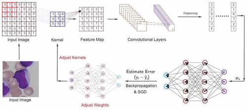
In this section, we briefly outline the methodology behind the considered approach². In the CNN³, the convolution operation of input data is performed with a feature detector/kernel. Each feature detector returns a feature map and each of these maps contains a key feature of a specific data point. Altogether the feature maps form a convolutional layer that summarizes the presence of features in an input image. An activation function, such as the Rectified Linear Unit (ReLU), is implemented to capture the non-linear features of the data. The output feature maps are usually sensitive to the location of the features in the input. Down-sampling or pooling techniques are called for to address such sensitivity and help in reducing the redundancy in features while still grasping the key properties of the data. These multi-dimensional pooled feature maps are then converted into one-dimensional arrays which are fed to fully connected neural networks by flattening the polled layers. From the beginning to this stage, we have transformed an image into a combination of vectors of numbers. Now, we initialize the NN by assigning random weights over each connection. Next, the data are fed to the succeeding layer for more modification. The network continues this procedure until it reaches the output layer and makes a prediction. After that, it estimates the error and backpropagates the error information. During the backpropagation, the network measures the contribution of kernels and weights to the loss function by stochastic gradient descent. Finally, the network adjusts the kernels as well as the weights and repeats these steps for a specific number of iterations, and in each iteration it minimizes the error function $\mathcal{L}$. In Figure 1, the learning mechanism has been graphically presented.

Figure 1. Architecture of Convolutional Neural Networks. Input images are at first, transformed into convolutional Layers. Each Feature Map in the Convolutional Layers is then flattened and forwarded to the NN. The Output Layer returns an estimated value of $y_i$, i.e., ${\hat{y}}_i$. Then we estimate the error, backpropagate the error information through network, and adjust the weights as well as the kernels based on their contribution to the loss function $\mathcal{L}$. The contribution to the loss is determined by mini-batch stochastic gradient descent. We repeat this process for a specific number of epochs/iterations until the loss function $\mathcal{L}$ is minimized.

Note that the traditional CNNs are prone to overfit unless we have a sufficiently big dataset. However, this problem can be tackled by implementing the Bayesian approach in CNN setup, originally proposed by Gal and Ghahramani (Gal and Ghahramani, 2016a). With this implementation, the model tries to reduce overfitting even on a small data while still provides the uncertainty estimates in CNNs (Gal and Ghahramani Gal and Ghahramani, 2016a). The usual Bayesian NNs offer a probabilistic interpretation of deep learning models by inferring distributions over the models’ weights. However, modeling with a prior distribution over the kernels (such as the one in the context of CNN) has never been attempted successfully before until recently by Gal and Ghahramani (Gal and Ghahramani, 2016a).

Given the dataset $X=x_i$ and its corresponding label set $Y$, in a classical setting, the CNN maps the input $x_i$ to the output $Y$ using the set of weights $\omega$. The resulting model can therefore be seen as a probabilistic model, where the output $p(y|x,\omega )$ is a categorical distribution. By placing a prior $p(\omega )$ over the kernels, the CNN can be converted to a Bayesian CNN. After setting the prior distribution over kernels, the posterior distribution becomes as follows:

(1) $p(\omega |X,Y)=\frac{p(Y|\omega ,X)p(\omega )}{p(Y|X)}\cdot$(1)

The presence of normalizing constant, $p(Y|X)$ in Equation (1)(1) $p(\omega |X,Y)=\frac{p(Y|\omega ,X)p(\omega )}{p(Y|X)}\cdot$(1) makes it difficult to estimate the posterior distribution of kernels and therefore Variational Inference (VI) is called for an approximation. With the VI technique, the true posterior distribution with a rather simpler variational distribution is approximated by minimizing the Kullback-Leibler (KL) divergence. Upon obtaining the approximate posterior distribution by VI, now we can estimate the predictive distribution by using the approximate posterior distribution together with MC integration as

$p(y^{\ast }|x^{\ast },X,Y)\approx \int p(y^{\ast }|x^{\ast },\omega )q(\omega |\theta )d\omega \approx \frac{1}{T}\sum _{t=1}^{T}p(y^{\ast }|x^{\ast },{\hat{\omega }}_t)$

where ${\hat{\omega }}_t$ is the sample of parameters drawn from the approximate posterior distribution $q(\omega |\theta )$. The traditional Bayesian NN models involve the Gaussian distribution as the a variational distribution, which makes the estimation process computationally expensive due to the high number of model parameters without contributing to the improvement of model performance (Blundell et al. 2015). To address that we follow the direction of Gal and Ghahramani (Gal and Ghahramani, 2016a), where the authors instead proposed Bernoulli distribution as variational distribution which requires no additional parameters for approximating the true posterior. This in turn makes the estimation of posterior distribution less computationally expensive and produces coherent outcomes. Another advantage with Bayesian models is that it offers a mathematical framework to reason about model uncertainty, but it comes with an enormous computational cost.

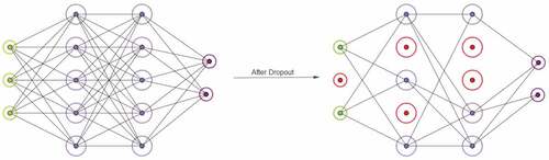
Dropout is a stochastic regularization technique that addresses the problem of overfitting and, therefore, reduces the computational complexity (Hinton, Srivastava, and Krizhevsky et al. (Hinton, et al., 2012a); Srivastava, Hinton, and Krizhevsky et al. 2014). With the dropout technique, during the training phase, some units from the networks are randomly neglected, which in consequence, reduces the number of parameters and makes the networks with less available amount of parameter to fit the data. With this technique, a unit is kept in the network with probability $p$ or omitted with probability $1-p$ (see Figure 2 for illustration). Let us consider an NN with $L$ layers and cross-entropy being the loss function. At the $i$th layers the weight matrices $W_i$ has the dimension $K_i\times K_{i-1}$ and the vector of bias $b_i$ has dimension $K_i$. Also, we consider $x_i$ as input which is an independent variable and $y_i$ being the output, a dependent variable for $i=1,2,\dots ,N$ observations. The cross-entropy function estimates the error, i.e., the difference between $y_i$ and ${\hat{y}}_i$. In general, to prevent NN from being overfitted due to a large number of the parameter we introduce a regularization term with the loss function. Here, we consider ridge regression or $L2$ regularization term in all layers with regularization parameter $\lambda$ dictating the magnitude of regularization (Tikhonov 1963). The optimization objective in NN with dropout then takes the form as,

${\mathcal{L}}_{DO}=\mathrm{L}\mathrm{o}\mathrm{s}\mathrm{s}\mathrm{f}\mathrm{u}\mathrm{n}\mathrm{c}\mathrm{t}\mathrm{i}\mathrm{o}\mathrm{n}+L_2\mathrm{R}\mathrm{e}\mathrm{g}\mathrm{u}\mathrm{l}\mathrm{a}\mathrm{r}\mathrm{i}\mathrm{z}\mathrm{a}\mathrm{t}\mathrm{i}\mathrm{o}\mathrm{n}$

(2) $=-\frac{1}{N}\sum _{i=1}^N[y_i\cdot log({\hat{y}}_i)+(1-y_i)\cdot log(1-{\hat{y}}_i)]+\lambda \sum _{i=1}^L(||W_i|{|}_2^2+||b_i|{|}_2^2).$(2)

Figure 2. On the left, fully connected Neural Networks with two hidden layers. On the right, Neural Networks after dropping out units at the input layer as well as hidden layers (red circled units). The networks now have less number of parameters to adapt to the dataset which in turn forces the networks to learn the relationship between independent variables and dependent variables more appropriately. This ”appropriate” learning reduces the risk of overfitting.

The same mechanism of dropout can be connected under the paradigm of BCNN. In fact, in Gal and Ghahramani (Gal and Ghahramani, 2016b), the authors show that the dropout networks’ training can be formulated as approximate Bernoulli variational inference in Bayesian NNs. In this way, the implementation of the Bayesian neural network during the training phase is reduced to performing dropout after every convolution layer. Due to the computationally ease it provides, in our work, we utilized the dropout to approximate the Variational Inference in BCNN.

Data

In this article, we implement this model on the microscopic images of blood samples obtained by using an optical laboratory microscope mounted on a Canon PowerShot G5 camera and sampled for ALL diagnosis. The acute lymphoblastic leukemia image database ALL-IDB has been used for the empirical study. ALL-IDB is a public image dataset of peripheral blood samples from normal individuals and leukemia patients, and it contains the relative supervised classification and segmentation data. These samples were collected by the experts at the M. Tettamanti Research Center for childhood leukemia and hematological diseases, Monza, Italy. The database has two distinct versions: the first version (ALL-IDB1) contains a dataset of 108 images with 39,000 blood elements and can be used for both testing the segmentation capability of algorithms, as well as the classification systems and image pre-processing methods, while the second version (ALL-IDB2), which contains 260 colored images of lymphocytes, is a collection of cropped areas of interest from normal and blast cells that belong to the ALL-IDB1 dataset, so it can be used only for testing the performance of classification systems. In this article, we used the ALL-IDB2 dataset for experiments in BCNN. A lymphocyte that is not cancerous is labeled as 0 and 1 represents a cancerous lymphocyte. All the images labeled as Y = 0 are obtained from healthy personals while Y = 1 labeled images were collected from ALL patients (Scotti (2005); Labati, Piuri, and Scotti 2011).

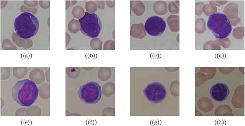
Sample images are plotted in Figure 3 with cancerous and noncancerous cells. The colored images are our input data and to be more specific, the pixel values of each image are the values of independent variables while the labels Y = 0 and 1 are classes of the dependent variable. Thus, we classify the images based on two classes. We train the model that can classify each of the lymphocyte cells previously labeled by expert oncologists.

Figure 3. Sample images from ALL-IDB1 dataset. First four lymphocytes (a – d) are cancerous while the remaining lymphocytes (e – h) are not. Lymphocyte cells are classified by expect oncologists.

To implement the BCNN approach, images are split as cancerous and noncancerous cells. Among 130 cancerous cells images, first 100 images are used in the training set, next 15 images are used in the validation set, and the last 15 images are used in the test set. In a similar manner, we split the 130 noncancerous cell images. As for the validation of results, the hold-out validation approach is used.

Result

This section summarizes the results obtained during the analysis. Six⁴ network structures are presented here and the results are summarized in Table 1. First, we display the accuracy rate returned by models from each network in our experiments and then, the predictive uncertainty produced by the best network is discussed. Finally, we check for overfitting for all models.

Table 1. Mean and Standard Deviation of models from six different network structures. Each network was tested 10 times to obtain the variation in model performance. The models trained in NN with 3 convolutional layers and 5 hidden layers produced the highest mean accuracy rate as well as lowest standard deviation of accuracy rate

Models	Accuracy Rate (Mean)	Accuracy Rate (SD)
3 Convolutional & 4 Hidden	89.33	14.35
3 Convolutional & 5 Hidden	94.00	2.00
4 Convolutional & 4 Hidden	90.79	7.39
4 Convolutional & 5 Hidden	93.41	2.93
5 Convolutional & 1 Hidden	78.63	6.09
5 Convolutional & 2 Hidden	88.12	12.15

Model performance

We experimented with several network architectures to find the model that produces the optimum result. During the training phase, we add a dropout layer after each convolutional layer as well as fully connected layers. For keeping the consistency, in all experimental models, the dropout rate after each convolutional layer is 20% while it is 50% for all fully connected layers. The reason behind taking the dropout rate as 20% was not to lose too much information while we implement the Bayesian CNN. Since the pooling operation makes the data compressed, taking a high dropout rate after the convolutional layer may put a heavy constraint on the learning process of the models. With $N$ refers to number of layers in different network structures, we experimented with 3 convolutional layers & 4 hidden layers, 3 convolutional layers & 5 hidden layers, 4 convolutional layers & 4 hidden layers, 4 convolutional layers & 5 hidden layers, 5 convolutional layers & 1 hidden layer and 5 convolutional layers & 2 hidden layers. We trained 10 different models for each of the network structures that we mentioned above with implementing dropout in each of the models. The loss function/objective function we deployed during the model training was binary cross-entropy since we are dealing with a two-class classification problem. For gradient descent optimization, initially, we experimented with different optimizers, e.g., adagrad, RMSprop, adamax, etc. and finally chose to deploy RMSprop as the final optimizer. The hyperparameter, learning rate in RMSpropoptimizer also experimented for different values, such as $0.001,0.002,0.005$ etc. We observe that the learning rate $0.0001$ was producing better results for our dataset and thus we keep that rate throughout all other models. Another hyperparameter of the RMSprop optimizer is the decay rate which was kept constant at $0.9$.

In the experimental setup, we trained our models with 200 images, while 30 images were kept for validation, and the remaining 30 for the testing phase. Each of the models was trained with 50 epochs, i.e., we passed the entire training set through the neural network 50 times. We used a mini-batch image size of 20, thus the steps per epochs were 10 for 200 images. During training, after each epoch, the network evaluates its learning process against the validation dataset. We shuffled the images within the validation dataset after each epoch. After training a model, we evaluated its performance on test data.

R programming language (RStudio) is used to implement BCNN in our dataset. TensorFlow, the most commonly used framework for Deep Learning is used to perform the tasks with Keras as API on top of Tensorflow (both are originally developed by Google). A computer with CPU configuration of Intel Core i5 4570@ 3.20 GHz and 8.00 GB Single-Channel DDR3 RAM is used to run the experiments.

The implementation of Bayesian CNN was done by 50 forward passes through the models while keeping the dropout active. We observe that, during the test time with MC dropout, the error rate varies from little to relatively large quantity depending on network structures. To obtain a reliable estimate, the process is repeated several times. Due to that, the MC dropout testing is repeated 10 times for each network and the mean and standard deviation of the accuracy rates are observed. Following table shows the accuracy rate in six different BCNN structures for 10 repetitions. As can be seen that, the chosen models provide a reliable accuracy rate for up to almost 94%, which is an incredible performance. Without any manual feature extraction, which is very common in such studies, all our proposed models manage to classify the correct image with around 90% accuracy, with an exception of 5 Convolutional 1 Hidden layer model. However, some models do produce a high standard deviation, which indeed shows high uncertainties, but the 3 Convolutional 5 Hidden layer and 4 Convolutional 5 Hidden layer models are found to be the best models with standard deviation in accuracy hovering around 2.

SD, Standard Deviation.

In the next table, we present results about the sensitivity and specificity returned by models from six different network structures. Table 2 shows the mean sensitivity and specificity with relative standard deviation for 10 models from each of these six network structures. From Table 2, we can observe again that models from 3 Convolutional & 5 hidden layers and 4 Convolutional & 5 hidden layers have obtained same specificity, and it turns out to be higher than other models. This indicates that models from these two networks have predicted the cancerous lymphocytes with high mean accuracy and low standard deviation compared to other models. While for the other models, the mean sensitivity and specificity results are very good but with high uncertainty and therefore, relying on these models can be misleading. Note that similar dataset has been used in Rawat et al. (2017); Putzu, Caocci, and Di Ruberto (2014); Genovese et al. (2021a), where features of interests were first extracted from the images through different image processing techniques, and then several classifiers are implemented to evaluate the classification accuracy. The resulting overall classification accuracy reported in these studies are not much different (94.5% and 93%, respectively)⁵ from what we obtained in this study without involving image processing methods. Here, we rely on the strength of Bayesian driven convolution neural network not only for classification but to self extract features from the images. Considering specificity as a performance measure, our approach outperforms findings reported in, such as Das and Meher (2021a) and Genovese et al. (Genovese, et al., 2021b). Besides these, since the Bayesian approach allows to evaluate model prediction uncertainty, our contribution provides more reliable estimate in comparison to existing studies.

Table 2. Mean and standard deviation of sensitivity and specificity returned by 10 models from each of six different network structures

	Sensitivity		Specificity
Models	Mean	SD	Mean	SD
3 Convolutional & 4 hidden	89.63	9.51	97.03	4.08
3 Convolutional & 5 hidden	89.33	5.62	99.33	2.11
4 Convolutional & 4 hidden	86.66	14.74	95.33	12.59
4 Convolutional & 5 hidden	88.67	6.32	99.33	2.11
5 Convolutional & 1 hidden	60.66	17.34	96.67	7.20
5 Convolutional & 2 hidden	81.33	25.30	96.67	8.46

SD, Standard Deviation.

We then move on further with the aim of understanding the dynamic structure of standard deviation of error rates obtained from different models. It is important since minimum error with consistent variation leads to reliable estimates. This is also useful to understand the model’s capability of making consistent predictions. In Figure 4, we graphically illustrate model performance for all of these different networks, where error rate produced by models from six different networks are plotted. Data was passed through the networks 50 times as depicted on the x-axis and the process was repeated 10 times producing the variation on the y-axis. Deep blue dots are the mean of error rates in 10 iterations and the error bars show the 1 standard deviation from the mean.

Figure 4. Error rate produced by models from six different networks. Data was passed through the networks 50 times as depicted on the x-axis and the process was repeated 10 times producing the variation on the y-axis. Deep blue dots are the mean of error rates in 10 iterations and the error bars show the 1 standard deviation from the mean.

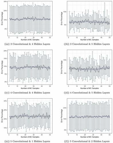
Here, the dynamic structure tells a better story about the variation. The mean of error rates is lowest with relatively smaller standard deviation for models with 3 convolutional & 5 hidden layers. Other models except the models trained on 4 convolutional layers and 5 hidden layers returned relatively higher error rates with very high standard deviation. For the best model structure which is 3 convolution and 5 hidden layers, we briefly provide some technical details. In the first convolution layer, the number of output filters is 32 and the kernel size is $3\times 3$ which refers to width and height on 2D convolution window. In the max-pooling layer, the pool size is $2\times 2$ which refers to the magnitude of downscaling. In the second and third convolution layers, the number of output filters is 64 and the kernel size is $3\times 3$. The max-pooling layer is kept the same as before, $2\times 2$. Next, in all 5 hidden layers, the number of nodes is 1024. The activation function in 3 convolution and 5 hidden layers are RELU while, in the output layer, the activation function is sigmoid.

Predictive uncertainty

For a binary classification problem, deterministic deep learning models produce a single probability value in favor of a class given an observation. But to capture the predictive uncertainty, one needs a distribution for each prediction rather than a point estimate. Within the BCNN structure we have such a facility and to obtain the predictive uncertainty for our model, we pass the data through the network 50 times during the testing period. This, in turn, produces a distribution of probabilities for each outcome given the input data. We take the MC dropout as the average of 50 probability values given an observation, the variation among these values provides the uncertainty estimates for each prediction made by the model.

Following this procedure, the estimation of predictive uncertainty is performed for all models from all networks. However, for brevity, in this section, we only focus on models from networks that returned the lowest error rates. From our experiment, the models from 3 convolutional layers & 5 hidden layers and 4 convolutional layers & 5 hidden layers produced the low error rates among all models as can be seen in Figure 4. Thus in the following, we discuss the predictive uncertainty for these two networks for which the results are presented in Figure 5 and Figure 6.

Figure 5. An illustration of predictive uncertainties returned by first four models trained on 3 convolutional layers and 5 hidden layers.

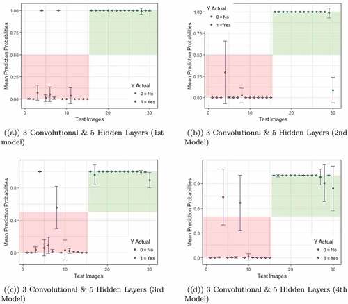
Figure 6. Predictive Uncertainty estimated by the first four models from network with 4 convolutional layers and 5 hidden layers.

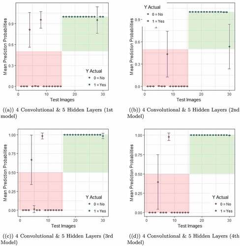
In the test data, first 15 images were labeled as 0, i.e., images with no sign of Leukemia and the remaining images were labeled as 1, i.e., images with the sign of Leukemia. If classified accurately, the predicted probabilities for images labeled as 0 should fall within the light red zone, while it is the light green zone for images labeled as 1. For instance, if an image from first 15 images is predicted wrongly, the probability value will fall outside of the red zone (top left white space). During the test time, a model produced the probability of a lymphocyte cell belonging to class ”1” given new input data. For each of the 30 test images, during test time we have produced 50 probability values by passing the data 50 times through each network and obtained a distribution of predicted probabilities for each image. Thus the orange and green dots are the mean of predicted probability values for classes 0 & 1, respectively and the error bars show one standard deviation of predicted probabilities.

Note that, due to the dropout each time the networks are different. The lower bound and the upper bounds for each image are defined by the mean of predicted probabilities $\pm$ one standard deviation of predicted probabilities from the mean. As can be seen from the graphs and through the orange and green dots, most of the times, the model correctly classify the correct image with a very low misclassification rate.

Overfitting

The curse of overfitting limits the applicability of traditional machine and deep learning approaches in many instances. Therefore, for the reliability of our approach, it is important to identify whether our approach is trapped by this curse or not. To do so, we extend the scope of analysis in this direction. For each of the six different CNN structures, during the training, we evaluated model performance on validation dataset and during the testing, we assessed the model performance on the test dataset. When a model gives relatively low error rate for validation dataset compared to the test dataset, it gives an indication of overfitting of the model. To identify it, we experimented it with all six network structures and repeated each structure 10 times. Thus, in total, we get 60 models and for brevity⁶, one model from each of the network structure is presented in Figure 7. This figure shows the performance of the models during the training and testing period. In the x-axis, we plot the epochs or iterations, while the y-axis presents the accuracy rate. The test accuracy rate is marked in red while the validation accuracy rate is marked in green. As can be seen immediately from Figure 7, the models based on 3 convolutional layers & 4 hidden layers, 3 convolutional layers & 5 hidden layers, 4 convolutional layers & 4 hidden layers and 4 convolutional layers & 5 hidden layers present similar pattern while for models based on 5 convolutional layers & 1 hidden layers and 5 convolutional layers & 2 hidden layers, the results are very different.

Figure 7. The figure shows the performance of the models during training and testing period. The first four plots (a,b,c,d) avoided the overfitting while the remaining two (e,f) show overfitting.

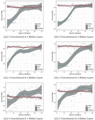
The validation accuracy rate (green line) for one of the models from first network (3 convolutional layers & 4 hidden layers), as in Figure 7(a) was below 0.5 when the model started its learning process. After around 35 epochs, the validation accuracy reached 90% and remained constant for the rest of the epochs. During the test time, the accuracy remained constant at 90% throughout 50 Monte Carlo iterations. Both test accuracy and validation accuracy merged after around 35 epochs/iterations and maintained this consistency for the remaining epochs/iterations. Models from 3 convolutional layers & 5 hidden layers (in Figure 7(b)) show more or less a similar pattern. Models trained in 4 convolutional layers & 4 hidden layers and 4 convolutional layers & 5 hidden layers, i.e., plot (c) & (d) in Figure 7 demonstrate the consistency in validation and test accuracy but here it was achieved at around 50 epochs. This consistency in validation accuracy and test accuracy indicates that the specific model from that network is not overfitting.

While for the case of models based on 5 convolutional layers & 1 hidden layers and 5 convolutional layers & 2 hidden layers, it is observable that the validation accuracy rates are exceeding the test accuracy after around 15 epochs/iterations and 25 epochs/iterations, as depicted in Figure 7(e) and Figure 7(f), respectively. Thus, it is conclusive that these models are overfitting the data and not suitable to be used for further analysis.

Discussion & conclusion

In this work, we have demonstrated how Bayesian CNN models can be implemented for classifying the cancerous and noncancerous lymphoblast cells and provide uncertainty estimates with their predictions. It contributes to the current literature related to the investigation of leukemia cancer cells, in particular, with an in-depth discussion on classification accuracy and prediction uncertainties, and application and interpretation of such model for image classification, in general. For the readers, we briefly provide an outline of the proposed method and summarized the mechanism with brevity. In the empirical study, the predictive models in BCNN structure are then implemented for ALL image classification. We show how a probabilistic model can be used for image classification with reasonably good classification accuracy, without manual or computer-aided feature extraction. Not only that, we further move on to obtain uncertainty estimates for the classification of each image, which is usually not discussed in existing studies. To obtain reliable predictions, we take the Bayesian approach in CNN, which in turn produces a distribution of probable output values given new inputs. The common problem of overfitting is discussed and, through illustration, it has been concluded that the chosen models do not overfit the data. This is important to highlight here because existing studies merely focus on classification accuracy and not much attention is usually given to such investigations.

Our experimentation with the image dataset for ALL image classification produced reliable results. In total, we develop models in six different network structures and for each structure the experiment is repeated 10 times to obtain the variation the models produced in predictions. The highest mean accuracy rate, obtained for the model with 3 convolutional layers and 5 hidden layers with mean accuracy (specificity) rate as 94% (99.3%) and with an SD deviation of 2. Together with the supporting evidence obtained from classification accuracy, prediction uncertainty, and overfitting estimates, we are certain that the models considered in these experiments can be deployed in classifying the microscopic lymphocyte cells with more reliability and for better diagnosis of ALL.

Future directions

In the future we aim to employ different DL architectures and databases with more samples to better assess the data. For small datasets, like the one used in the study, active learning can be implemented for better classification. In Active Learning, all the data points are not required to be labeled when we start training our model, rather the algorithm starts with very small data and during the learning process, the model itself asks the user (human expert) to label a specific data point if needed. With the Bayesian approach and Active Learning, one can classify the microscopic images of lymphocyte cells and obtain not only the predictions accuracies, but the predictive uncertainty as well, which is more reliable while avoiding overfitting at the same time. Moreover, to further reduce the computational efficiency of the employed approach, Bayesian CNN can be coupled with, such as transfer learning, factorization/decomposition of convolution kernels, and depthwise separable convolutions approaches with more up-to-date visualizations approaches, such as t-sne. In this article, we stick to the most commonly used performance assessment criteria, such as the accuracy, specificity, and sensitivity complemented with overfitting analysis, but other approaches, such as precision and F1 Score can also be implemented to compare performance analysis.

Acknowledgments

Farrukh Javed acknowledges financial support from the internal research grants at Örebro University.

Data Availability Statement

The data that support the findings of this study are openly available in [repository: ALL_IDB] and can be accessed at https://homes.di.unimi.it/scotti/all/.

Disclosure statement

No potential conflict of interest was reported by the author(s).

Supplemental data

Supplemental data for this article can be accessed on the publisher’s website.

Notes

1. In McLachlan et al. (2020), the authors summarized the Bayesian approaches used in healthcare in producing meaningful and accurate decision-support systems.

2. For more technical details, we suggest readers to please refer to the references therein.

3. See Goodfellow, Bengio, and Courville (2016) for details.

4. Several networks are tested during the process but based on the performances, only six networks are kept for the rest of the analysis.

5. We report the highest reported overall accuracy here. For detailed results, we refer the readers to Rawat et al. (2017); Putzu, Caocci, and Di Ruberto (2014).

6. Note that all other models from respective network structures showed almost a similar performance with slight deviations.

References

- Amin, M. M., S. Kermani, A. Talebi, and M. G. Oghli. 2015. Recognition of acute lymphoblastic leukemia cells in microscopic images using k-means clustering and support vector machine classifier. Journal of Medical Signals and Sensors 5 (1):49. doi:10.4103/2228-7477.150428.
- Angermueller, C., T. Parnamaa, L. Parts, and O. Stegle. 2016. Deep learning for computational biology. Molecular Systems Biology 12 (878):1–866. doi:10.15252/msb.20156651.
- Bardou, D., K. Zhang, and S. M. Ahmad. 2018. Lung sounds classification using convolutional neural networks. Artificial Intelligence in Medicine 88:58–69. doi:10.1016/j.artmed.2018.04.008.
- Blundell, C., J. Cornebise, K. Kavukcuoglu, and D. Wierstra (2015). Weight uncertainty in neural networks. In Proceedings of the 32Nd International Conference on International Conference on Machine Learning - Volume 37, ICML’15, Lille, France, 2015, pp. 1613–22. JMLR.org.
- Butler, K. T., D. W. Davies, H. Cartwright, O. Isayev, A. Walsh, et al. 2018. Machine learning for molecular and materials science. Nature. 559(7715):547–55. doi:10.1038/s41586-018-0337-2.
- Das, P. K., A. Pradhan, and S. Meher. 2021. Detection of acute lymphoblastic leukemia using machine learning techniques. In Machine Learning, Deep Learning and Computational Intelligence for Wireless Communication. Lecture Notes in Electrical Engineering, ed. E. S. Gopi, vol. 749, 25–437. Singapore: Springer.
- Das, P. K., and S. Meher. 2021a. An efficient deep convolutional neural network based detection and classification of acute lymphoblastic leukemia. Expert Systems with Applications 183:115311. doi:10.1016/j.eswa.2021.115311.
- Das, P. K., and S. Meher 2021b. Transfer learning-based automatic detection of acute lymphocytic leukemia. National Conference on Communications (NCC), 1–6.
- Das, P. K., S. Meher, R. Panda, and A. Abraham. 2020. A review of automated methods for the detection of sickle cell disease. IEEE Reviews in Biomedical Engineering 13 309–324.
- Das, P. K., S. Meher, R. Panda, and A. Abraham. 2021. An efficient blood-cell segmentation for the detection of hematological disorders. IEEE Transactions on Cybernetics 1–12. doi:10.1109/TCYB.2021.3062152.
- Das, P., K. Jadoun, and S. Meher 2020.Detection and classification of acute lymphocytic leukemia EEE-HYDCON, 1–5.
- Gal, Y., and Z. Ghahramani 2016a. Bayesian convolutional neural networks with Bernoulli approximate variational inference. In 4th International Conference on Learning Representations (ICLR) Caribe Hilton, San Juan, Puerto Rico.
- Gal, Y., and Z. Ghahramani 2016b. Dropout as a Bayesian approximation: Representing model uncertainty in deep learning. In Proceedings of the 33rd International Conference on Machine Learning, New York, NY, USA, 2016, 1050–59.
- Genovese, A., M. S. Hosseini, V. Piuri, K. N. Plataniotis, and F. Scotti 2021a. Acute Lymphoblastic Leukemia detection based on adaptive unsharpening and Deep Learning. In Proc. of the 2021 IEEE Int. Conf. on Acoustics, Speech, and Signal Processing (ICASSP 2021), Toronto, ON, Canada, June 6-11, 2021, 1205–09.
- Genovese, A., M. S. Hosseini, V. Piuri, K. N. Plataniotis, and F. Scotti 2021b. Histopathological transfer learning for Acute Lymphoblastic Leukemia detection. In Proc. of the 2021 IEEE Int. Conf. on Computational Intelligence and Virtual Environments for Measurement Systems and Applications (CIVEMSA 2021), June 18-20, 2021 Hong Kong, China, 1–6.
- Goodfellow, I., Y. Bengio, and A. Courville. 2016. Deep learning, vol. 1. Cambridge, MA,: MIT press Cambridge.
- Hinton, G. E., N. Srivastava, A. Krizhevsky, Ilya Sutskever, I., Salakhutdinov, R. R., et al. 2012a. Improving neural networks by preventing co-adaptation of feature detectors. arXiv preprint arXiv:1207.0580.
- Hinton, G., N. Srivastava, and K. Swersky. 2012b. Neural networks for machine learning. https://www.cs.toronto.edu/tijmen/csc321/slides/lecture_slides_lec6.pdf.
- Hunger, S. P., C. G. Mullighan, and D. L. Longo. 2015. Acute lymphoblastic leukemia in children. New England Journal of Medicine 373 (16):1541–52. doi:10.1056/NEJMra1400972.
- Husham, A., M. H. Alkawaz, T. Saba, A. Rehman, J. Saleh Alghamdi, et al. 2016. Automated nuclei segmentation of malignant using level sets. Microscopy Research and Technique. 79(10):993–97. doi:10.1002/jemt.22733.
- Iqbal, S., M. U. Ghani, T. Saba, A. Rehman, and P. Saggau. 2018. Brain tumor segmentation in multi-spectral MRI using convolutional neural networks (CNN). Microscopy Research and Technique 81 (4):419–27. doi:10.1002/jemt.22994.
- Labati, R. D., V. Piuri, and F. Scotti. 2011. All-idb: The acute lymphoblastic leukemia image database for image processing. In 18th IEEE international conference on Image processing (ICIP), 2011 Brussels, Belgium, 2045–48.
- LeCun, Y., Y. Bengio, and G. Hinton. 2015. Deep learning. Nature 521 (7553):436–44. doi:10.1038/nature14539.
- Li, J., M. Gao, R. D'Agostino, et al. 2020. Evaluating classification accuracy for modern learning approaches. Cell. 180(4):688–702. doi:10.1016/j.cell.2020.01.021.
- Li, J., M. Gao, and R. D’Agostino. 2019. Evaluating classification accuracy for modern learning approaches. Statistics in Medicine 38 (13):2477–503. doi:10.1002/sim.8103.
- Masud, M., A. Eldin Rashed, and M. Hossain. 2020. Convolutional neural network-based models for diagnosis of breast cancer. Neural Computing and Applications 1–12.
- McLachlan, S., K. Dube, G. A. Hitman, N. E. Fenton, E. Kyrimi, et al. 2020. Bayesian networks in healthcare: Distribution by medical condition. Artificial Intelligence in Medicine 107:101912. doi:10.1016/j.artmed.2020.101912.
- Mohapatra, S., D. Patra, and S. Satpathy. 2014. An ensemble classifier system for early diagnosis of acute lymphoblastic leukemia in blood microscopic images. Neural Computing & Applications 24 (7–8):1887–904. doi:10.1007/s00521-013-1438-3.
- MoradiAmin, M., A. Memari, N. Samadzadehaghdam, S. Kermani, A. Talebi, et al. 2016. Computer aided detection and classification of acute lymphoblastic leukemia cell subtypes based on microscopic image analysis. Microscopy Research and Technique. 79(10):908–16. doi:10.1002/jemt.22718.
- NCI. 2018. National Cancer Institute U.S.A.
- Putzu, L., G. Caocci, and C. Di Ruberto. 2014. Leucocyte classification for leukaemia detection using image processing techniques. Artificial Intelligence in Medicine 62 (3):179–91. doi:10.1016/j.artmed.2014.09.002.
- Rawat, J., A. Singh, H. S. Bhadauria, J. Virmani, J. S. Devgun, et al. 2017. Classification of acute lymphoblastic leukaemia using hybrid hierarchical classifiers. Multimedia Tools and Applications. 76(18):19057–85. doi:10.1007/s11042-017-4478-3.
- Scotti, F. 2005. Automatic morphological analysis for acute leukemia identification in peripheral blood microscope images. In IEEE International Conference on Computational Intelligence for Measurement Systems and Applications, 2005, Messian, Italy, pp. 96–101.
- Singh, G., G. Bathla, and S. Kaur. 2016. Design of new architecture to detect leukemia cancer from medical images. International Journal of Applied Engineering Research 11 (10):7087–94.
- Srivastava, N., G. Hinton, A. Krizhevsky, Sutskever, I., Salakhutdinov, R., et al. 2014. Dropout: A simple way to prevent neural networks from overfitting. The Journal of Machine Learning Research 15 (1):1929–58.
- Steingrimsson, J. A., and S. Morrison. 2020. Deep learning for survival outcomes. Statistics in Medicine 39 (17):2339–49. doi:10.1002/sim.8542.
- Tikhonov, A. 1963. Solution of incorrectly formulated problems and the regularization method. Soviet Mathematics - Doklady 4:1035–38.
- Vos, T., C. Allen, M. Arora, R. M. Barber, et al. 2016. Global, regional, and national incidence, prevalence, and years lived with disability for 310 diseases and injuries, 1990–2015: A systematic analysis for the global burden of disease study 2015. The Lancet 388 (10053):1545–602.
- Zang, N., Y. Cia, Y. Wang, Y. Tian, X. Wang, and B. Badami. 2020. Skin cancer diagnosis based on optimized convolutional neural network. Artificial Intelligence in Medicine 102:1–7.