Evaluating the Efficacy of Small Face Recognition by Convolutional Neural Networks with Interpolation Based on Auto-adjusted Parameters and Transfer Learning

ABSTRACT

In this work, we propose a new approach for face recognition using low-resolution images. By cleverly combining conventional interpolation methods with the state-of-the-art classification approach, i.e. convolutional neural network, we introduce a new approach to efficiently leverage low-resolution images in classification task, especially in face recognition. Besides, we also do experiments on some recent popular methods, our approach outperforms some of them. Additionally, we propose a specific transfer learning strategy based on the preexisting well-known concept dedicated to low-resolution transfer learning. It boosts performance and reduces training time significantly. We also investigate on scalability by applying Bayesian optimization for hyper-parameter search. Therefore, our approach is able to be widely applied in many kinds of datasets and low-resolution classification tasks due to automatically seeking optimal hyper-parameters, which makes our method competitive to others.

Introduction

Image classification problem so far has many applications in the real world. Recently, most attentions focus on problems related to face recognition in business and security. For example, facial emotional recognition helps to investigate user’s behaviors in business (J. Chen et al. 2014), facial iris recognition is broadly applied for mobile security (Minaee and Abdolrashidi 2019). Besides, face recognition for surveillance is also significantly attractive, many approaches have been proposed which can be divided into learning and unlearning-based ones. In particular, popular methods of the later, including Local Binary Patterns (LBP) (Ojala, Pietikainen, and Maenpaa 2002) and Histograms of Oriented Gradients (HOG) (Dalal and Triggs 2005), use pre-defined filters to extract features by intention. These approaches were widely applied many years ago until the learning-based methods appear such as Principal Component Analysis (Wold, Esbensen, and Geladi 1987), Support Vector Machine (Suykens and Vandewalle 1999), and Convolutional Neural Network lately. AlexNet can be seen as the pioneer forming the baseline Convolutional Neural Network (CNN) architecture which surprisingly outperformed in image classification task (Krizhevsky, Sutskever, and Hinton 2012). Afterward, other popular CNN-based architectures such as VGG (Simonyan and Zisserman 2014), ResNet (He et al. 2016), DenseNet (Huang et al. 2017), etc, increasingly challenge most ever classification tasks.

Generally, in order to perform well in image classification, it requires a huge amount of high-resolution data. However, most real-world deep-learning-based applications suffer a significant challenge. Since images in the wild are often low-resolution, i.e. the resolution of captured image for inference is lower than training image, due to either far distance or bad quality of device. The problem can be resolved by transforming these images resolution to the original one thanks to conventional interpolation algorithms. However, this can lead to a bad quality result when inference image’s resolution is much lower than the original one (see Figure 1). As experiments by Li et al. have shown, small resolution images cause a significant downgrade of accuracy in prediction (Li et al. 2018). Additionally, they indicate that images, which resolution are lower than $16\times 16$ usually being ignored or thrown away. This leads to the waste of data and resources in some cases. Especially in crime tracking and recognition when all relevant data are vulnerable and should be utilized thoroughly.

Figure 1. Same image in different low resolutions (top), and their corresponding bilinear interpolated images (bottom). The recovered images of last two extremely low-resolution cases are nearly indistinguishable. Many works only handle low resolution up to $16\times 16$ while ours can handle even lower resolution images.

To address the problem, we aim to seek an efficient approach that is robust to low-resolution image classification. The proposed method should preserve the accuracy of it as much as possible. Particularly, given an original CNN-based model already trained on original high-resolution images, our method automatically produces optimal dimensions and CNN architectures, which are able to deal with any resolution. Moreover, we also introduce two optimizations for the problem that (i) accelerate the training time and performance, (ii) adapt various types of data by automatically searching for dedicated hyper-parameters. In summary, our contribution are as follows:

• We survey through many existing solutions for low-resolution recognition. These approaches vary from some conventional interpolations such as nearest neighbor, bi-linear, etc. to learning-based methods, i.e. Super Resolution Convolutional Neural Network and many state-of-the-art works.

• We propose an approach that significantly surpasses other methods. Our algorithm is a combination of deep learning and typical interpolation guiding the down-sampling process and modification of corresponding architecture.

• We further enhance the scalability to practically apply in various real-world problems. Particularly, the training time is reduced thanks to our block transfer learning, and flexible to apply in many different kinds of problems by leveraging Bayesian optimization (Snoek, Larochelle, and Adams 2012).

Our work is organized as follows. In Section 2, we survey some popular state-of-the-art approaches which currently handle the problem. In Section 3, our proposed method is introduced in detail. We conduct experiments and discussion in Section 4. Section 5 is the conclusion.

Related Work

To solve the image classification task in high dimension image data, many approaches are divided into manual-based and automated-based. For the manual ones, Local Binary Pattern (LBP) (Ojala, Pietikainen, and Maenpaa 2002) and Histograms of oriented gradients (HOG) features (Dalal and Triggs 2005) are considered as popular methods. These methods take advantage of pre-defined filters for the feature extraction phase, hence, require specific experiences to acquire good performance but are more computationally efficient instead. On the other hand, automated feature extraction methods represented by CNN-based are recently accounting for significant performance. The increasing complexity of datasets entails the deeper of CNN architecture. For example, the first version of VGG had 16 layers then increased to 19 layers (Simonyan and Zisserman 2014), ResNet (He et al. 2016), and DenseNet (Huang et al., 2017) with the same idea but were even deeper, they appended shortcut layers and a large number of trainable parameters. However, when dealing with low resolution images, the experiments show significant drops in accuracy of those architectures. Surprisingly, shallow models like AlexNet are more vulnerable to low image resolution compared with deep models like ResNet (Koziarski and Cyganek 2018). Since the convolved features completely flush out if a model is too deep. We claim that a model can keep performing well on low-resolution images by modifying its architecture based on the original one following our proposed transformation.

On the behalf of low-resolution image classification problem, especially in face recognition, the methods can be divided into two main approaches: interpolation-based and optimization-based.

Interpolation-based Methods

The main idea is to focus on how to preserve and restore from low-resolution image to the original one. In other words, one aims to restore an image $x$ with resolution $s$ back to $s_0$ $\left(s<s_0\right)$ by an interpolated function $\mathcal{I}\left(x,\theta \right)$, $\theta$ is set of parameters that produces $\hat{x}$. Hence, the restoration is equivalent to minimize the noise between original image $x$ and interpolated image $\hat{x}$ by a specific metric $d\left(x,\hat{x}\right)$, which is $\hat{\theta }=arg\underset{\theta }{min}d\left(x,\hat{x}\right)$ where $\hat{\theta }$ is optimal parameters. The $\theta$ significantly depends on $\mathcal{I}$. In particular, there are two approaches: conventional interpolation and deep learning enhancement.

Conventional Interpolation

$\mathcal{I}$ represents as approximation function, which is $\mathcal{I}\left(x,\theta \right)=x\ast h_{\theta }$, where $h_{\theta }$ denotes convolutional function. These approximation functions are obviously computational, since they pre-define $\theta$ before applying to interpolation. In fact, $\theta$ is practically chosen from experiments and fixed. Some popular approximation functions are nearest neighbor, bi-linear, bi-cubic, etc. As a result, they achieve affordable accuracy, but faster in return. Figure 2 shows the results from some conventional approximation functions.

Figure 2. Some well-known conventional interpolation methods. First image is the original, the rest are the interpolated ones.

Deep Learning Enhancement

In recent years, many kinds of research give efforts to overcome the disadvantage of conventional approaches. Unlike conventional interpolation fixing $\theta$, they integrate deep learning into account, which makes $\theta$ learnable. Dong et al. are succeeded in taking advantage of CNN and propose Super Resolution CNN (SRCNN) (Dong et al. 2015). Generally, the original SRCNN and its relative aim to learn the mapping function from low to high-resolution images. They first up-sample dimension of images to the original one using bicubic interpolation, then apply CNN architecture to learn the mapping function. Their experiments give a significant improvement evaluated on PSNR/SSIM assessments (Wang et al. 2004). However, SRCNN has difficulty dealing with extremely low dimension, since up-sampling to the original one with a large range causes vast amount of information leaks. This limitation is observed in Figure 3.Other architectures, such as Super-FAN (Bulat and Tzimiropoulos 2018) and FSRNet (Y. Chen et al. 2018), take advantage of GAN-based (Radford, Metz, and Chintala 2015) to be more generative when producing high resolution image. However, they are deep and complex. Additionally, GAN-based models are experimentally hard for training due to high computation and time-consuming.

Figure 3. Some interpolation results by SRCNN.

Optimization-based Methods

These works focus on directly optimizing $\theta$ existing low-resolution images without restoring to the original one. So far, neural architecture search (NAS) has much impact. Zoph et al. propose a reinforcement strategy to generate suitable architecture depending on data properties (Zoph and Le 2016). However, each kind of resolution requires a specific CNN architecture, which is impractical for applications in the wild.

Recently, there are many state-of-the-art works paying more attention to low resolution face recognition. A significant approach is taken knowledge distillation into account. One consists of two-stream networks denoted as teacher and student models, where the former one is large and deep while the later prefers much simpler and shallower. As a result, the student network can inherit the robust knowledge from the teacher one but still ensure the performance and simplicity. To enhance distilling effectively from robust and discriminative features, Ge et al. consider graph labeling problem based on sparse-connected constructed from face dataset (Ge et al. 2018). Their further work employs cross-dataset as a bridge of distillation, where the teacher model is trained on private high-resolution dataset and fine-tuned on the public one to preserve compact and discriminative features. The student model jointly learns to mimic the adapted high-resolution features and face classification on low-resolution dataset (Ge et al. 2020). Although these works perform well by inheriting robust knowledge from the teacher model, the student one is independently selected without considering the architecture of the former. Our method, on the other hand, proposes transformation function to construct the models for low-resolution images consistently based on the original one. Besides, other work combines the high and low-resolution images for training and identify discriminative features yet robust to resolution change. For instance, Deep Coupled Resnet consists of a trunk model followed by multi-branches learning three specific resolutions. The authors constrain the distance between high and low-resolution features by Coupled-Mapping loss so that model can learn robust features (Lu, Jiang, and Kot 2018). Other work also defines and trains network with many different levels of low resolution called PixelHop++ Y. Chen et al. 2020). It is leveraged to either construct successive subspace learning using different color channels (Rouhsedaghat et al. 2021b) or build a specific network on top of it, i.e. FaceHop (Rouhsedaghat et al. 2021a). We observe that our proposed method can perform well and show a considerably results on lower resolutions comparing to those experiments.

Hence, for the sake of taking advantage of both interpolation and optimization-based, we propose an efficient strategy to wisely produce optimal resolutions and corresponding CNN architectures. Whether the input image’s resolution is high, low, or extremely low, our algorithm can handle direct it to the desired model to achieve the best accuracy.

Method

Hypothesis

Intuitively, we believe that there are optimal resolutions, which come with corresponding optimal CNN architectures varying from high to low resolutions. These optimal resolutions and architectures should be consistent and formulated by our proposed architecture transforming function (ATF) and scale transforming function (STF), respectively.

As a result, our purpose is to form optimal ATF and STF formulas. The STF takes the input resolution, then generates ones varying in a wide range. Besides, the ATF takes the responsibility to generate optimal CNN architectures that satisfy the corresponding resolutions generated by STF. It takes the number of convolutional blocks of the original model, then calculates the optimal one to construct the model architecture for corresponding resolution produced by STF. In particular, the model becomes shallower (i.e. the number of convolutional blocks are decreased) in down-sampling process. After that, the original data are degraded to resulting resolutions and fed to models for training. For the inference phase, given an input image, we define a strategy to interpolate it to the appropriate resolution of trained CNN models.

Problem Definition

Given a single image $x$ with corresponding resolution $s=M\times N$. $M,N$ are the height and width of $x$, respectively. We denote set of data ${\mathcal{T}}_s=\left({\mathcal{X}}_s,{\mathcal{Y}}_s\right)$ which contains images ${\mathcal{X}}_s=\{x_0,x_1,\dots x_{N-1}{\}}_s$, and corresponding labels ${\mathcal{Y}}_s=\{y_0,y_1,\dots y_{N-1}{\}}_s$, $N$ is number of training data.

For an identical CNN architecture, we define it based on block unit where a single block is a structure containing some specific layers that repeat sequentially to form the feature extraction. Therefore, we denote a CNN architecture as $F\left(x,s,b\right)$ generated by input image $x$ with resolution $s$ and $b$ blocks. We define STF and ATF as $\varphi \left(s,{\theta }_s\right)$ and $\psi \left(b,{\theta }_b\right)$ where ${\theta }_s$ and ${\theta }_b$ are the adjusted hyper-parameters, respectively.

Given original data ${\mathcal{T}}_0$ and pre-trained model structured by architecture $F\left(x,s_0,b_0\right)$. Generally, we aim to produce set of data $\mathcal{P}=\left\{p_i\right\},i\in \left(0,T\right)$ where $T$ is pre-defined parameters, which is the number of datasets. $p_i=\left({\mathcal{T}}_{si},F\left(x,s_i,b_i\right)\right)$ is optimal pair of dataset and model generated by $\varphi \left(s,{\theta }_s\right)$ and $\psi \left(b,{\theta }_b\right)$, respectively. Our purpose is to find the optimal ${\theta }_s$ and ${\theta }_b$ that minimize the average loss from each $F\left(x,s_i,b_i\right)$ trained on ${\mathcal{T}}_{si}$ as follow:

(1) $\hat{\theta }=arg\underset{{\theta }_s,{\theta }_b}{min}\frac{1}{T}\sum _{i=0}^{T-1}\mathcal{L}\left(F\left(x,\varphi \left(s_i,{\theta }_s\right),\psi \left(b_i,{\theta }_b\right)\right)\right)$(1)

where $\hat{\theta }=\left\{\widehat{{\theta }_s},\widehat{{\theta }_b}\right\}$ and $\mathcal{L}\left(\cdot \right)$ denote the optimal hyper-parameters and the loss function of the model, respectively.

Training

Heuristically, $\varphi$ and $\psi$ are rarely applied for the original ${\mathcal{T}}_0$ and $F\left(x,s_0,b_0\right)$. In fact, we experiment that the original architecture $F\left(x,s_0,b_0\right)$ still gives the best performance, i.e small loss, for some first resolution scales until they reach a specific one, say $r$, that significantly raises the loss. As a result, it is worth finding $r$ as the input scale of ATF and STF. We would like to propose the algorithm seeking $r$ in Algorithm 1. In particular, our original data are down-sampled to specific resolution scales, and up-sampled again to the original $s_0$ by any conventional interpolation algorithm such as nearest neighbor, bi-linear, etc ($Down\mathrm{\_}ReupSample$ function). Then they are evaluated by $F\left(x,s_0,b_0\right)$. The scale which causes the most increasement of loss is marked as $r$. The process of down-sampling and up-sampling leads to information loss in the image. Hence, we can observe $F\left(x,s_0,b_0\right)$ can preserve the manners until which scale, we then mark $r$ as that one.

Alogrithm 1 Finding $r$

Input: ${\mathcal{T}}_0,s_0,F_0\left(b_0\right),T$

Output: $r$$i\leftarrow 0$$losses\leftarrow Empty,dists\leftarrow Empty${Evaluate on specific scales}

While $i<T-1$ do${\mathcal{T}}_i\leftarrow Down\mathrm{\_}ReupSample\left({\mathcal{T}}_0,0.5-i\right)$$loss\leftarrow \mathcal{L}\left(F_0\left(b_0\right),{\mathcal{T}}_i\right)$

Append $loss$ to $losses$$i\leftarrow i+1$

End while

{Get max distance of resulted losses}$i\leftarrow 0$

While $i<T-2$ do

Append $abs\left(acc\left(i+1\right)-acc\left(i\right)\right)$ to $dists$$i\leftarrow i+1$

End while$r\leftarrow argmax\left(dists\right)$

Return $r$

As being mentioned by our assumption, the resolution down-sampling process and modification of model’s architecture is relevant. We experiment that the transformation of resolution and corresponding CNN architecture strictly follow non-linear function, specifically exponential one. We propose the formula of STF and ATF as $\varphi$ and $\psi$, respectively,

(2) $\varphi \left(s,{\theta }_s\right)=\alpha \cdot s^{\beta }+\hspace{0.17em}{ }_s$(2)

(3) $\psi \left(b,{\theta }_b\right)=\gamma \cdot b^{\delta }+\hspace{0.17em}{ }_b$(3)

where

$\beta \in \left(0,1\right),\alpha \hspace{0.17em}lt;s^{1-\beta }-\hspace{0.17em}s{s}^{\beta },\delta \in \left(0,1\right),\gamma \hspace{0.17em}lt;b^{1-\delta }-\hspace{0.17em}b{b}^{\delta }$

${\theta }_s=\left\{\alpha ,\beta ,{ }_s\right\}$ and ${\theta }_b=\left\{\gamma ,\delta ,{ }_b\right\}$ are hyper-parameters. Those conditions ensure the down-sampling process, i.e output resolution is smaller than the input.

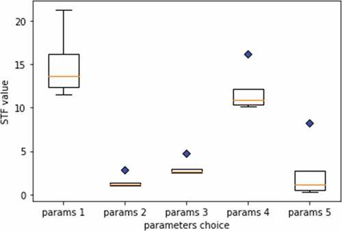
The choice of hyper-parameters of ATF and STF is crucial. Optimal hyper-parameters should help STF and ATF produce value varying in a wide range. For instance, Figure 4 shows the box plot of various parameters of STF. Particularly, the first one (params 1) is most optimal choice since its variance is greater than the rest and has no outlier.

Figure 4. The box plot represents the choices of STF’s hyper-parameters with 5 sets $\left(\alpha ,\beta \right)=\left\{\left(2.59,0.61\right),\left(1,0.3\right),\left(2,0.25\right),\left(4,0.4\right),\left(0.5,0.8\right)\right\}$ denoted as params 1 to params 5, respectively. The blue diamonds depict the outliers. Param 1 is the most optimal one since it has the largest variance without outlier.

Afterward, our transformation is conducted by $\varphi \left(s,{\theta }_s\right)$ and $\psi \left(b,{\theta }_b\right)$ with given ${\mathcal{T}}_r,F\left(x,s_0,b_0\right)$ where ${\mathcal{T}}_r$ is the set of data at scale $r$. In particular, we generate $T$ set of data and corresponding models, then the training process is applied. The algorithm is clearly defined in Algorithm 2. It produces sets of models with optimal scale $\mathcal{P}$.

Alogrithm 2 Training

Input: $\varphi \left(s,{\theta }_s\right),\psi \left(b,{\theta }_b\right),{\mathcal{T}}_r,F_0\left(b_0\right),T$

Output: $\mathcal{P}$$i\leftarrow 0,s\leftarrow GetSize\left({\mathcal{T}}_r\right),b\leftarrow b_0$$\mathcal{P}\leftarrow Empty$

{Loop through each dataset}

While $i<T$ do$s\leftarrow \varphi \left(s,{\theta }_s\right),b\leftarrow \psi \left(b,{\theta }_b\right)$

{Train}

repeat$Loss\left(F\left(s,b\right)\right)$$Optimize\left(F\left(s,b\right)\right)$

until converge

Append $F\left(s,b\right)$ to $\mathcal{P}$

End while

Return $\mathcal{P}$

Inference

Our proposed method in the training phase results in $\mathcal{P}$ set of data with optimal resolutions and corresponding trained models. In the inference phase, we take into account these resulted $\mathcal{P}$ dealing with any image resolution. In other words, giving an input image $\widehat{x_s}$ with resolution $\hat{s}$. Since $\hat{s}$ can be unequal to any dedicated one in $\mathcal{P}$, $\widehat{x_s}$ should be transformed into a specific optimal one in $\mathcal{P}$ which achieves the best accuracy. Let us introduce the strategy in Algorithm 3. We calculate the optimal model where its resolution is closest to one of $\widehat{x_s}$ using $GetNearest$ function. Then a conventional interpolation function $\mathcal{I}$ is applied, which takes consider image as input and produces output with the target resolution. Finally, the interpolated image is inferred by the corresponding model.

Alogrithm 3 Inference

Input: $\widehat{x_s},\mathcal{P}$

Output: label $l$, probability $p$$s,F\leftarrow GetNearest\left(\mathcal{P}\right)$$x_s^{\ast }\leftarrow \mathcal{I}\left(\widehat{x_s},s\right)l,$$p\leftarrow Predict\left(F,x_s^{\ast }\right)$

Return $l,p$

Optimization

The proposed method is able to deal with the variance of dimensions. However, there are some significant challenges.

Firstly, it mostly depends on $\varphi \left(s,{\theta }_s\right)$ and $\psi \left(b,{\theta }_b\right),$ especially are hyper-parameters ${\theta }_s$ and ${\theta }_b$ where they have to be pre-defined. In fact, these hyper-parameters are often variant. For instance, ones are effective in the face recognition but behave poorly in the dog vs cat classification with the identical values due to the difference in attribute and distribution of data. To strengthen automation capability, a search strategy is introduced. In general, grid search (LeCun et al. 2012) and random search (Bergstra and Bengio 2012a) are good choices in common due to their simplicity. However, they are exhaustive search strategies and only work well with a small number of hyper-parameters. Instead, we leverage another search algorithm based on Bayes theory, i.e Bayesian optimization Snoek, Larochelle, and Adams 2012), which is highly effective on large-scale number of hyper-parameters.

Secondly, the typical limitation of deep learning problem is exhausted training time. Deep models such as VGG (Simonyan and Zisserman 2014), ResNet (He et al. 2016), DenseNet (Huang et al. 2017) acquire a long training time since they deeply stack convolutional layer to effectively learn complicated features. Fortunately, this problem can be resolved by transfer learning (Weiss, Khoshgoftaar, and Wang 2016). For further improvement, we propose an effective transfer learning strategy based on underlying one called block transfer learning.

Bayesian Optimization

Our purpose is to seek optimal hyper-parameters for $\varphi \left(\cdot \right)$ and $\psi \left(\cdot \right),$ i.e. ${\theta }_s$ and ${\theta }_b$. Let us denote $\theta =\left\{{\theta }_s,{\theta }_b\right\}=\left\{\alpha ,\beta ,{ }_s,\gamma ,\delta ,{ }_b\right\}$ as set of hyper-parameters. We then apply bayesian optimization to find optimial $\hat{\theta }$ minimizing average loss, or maximizing average accuracy of all models produced by $\varphi \left(\cdot \right)$ and $\psi \left(\cdot \right)$. Formally, the method optimizes on the function level. Instead of directly optimizing an expensive objective function, i.e. hyper-parameters tuning for deep learning model, we define a surrogate model, which is cheaper than the original one that follows the normal distribution (Snoek, Larochelle, and Adams 2012). Particularly, the surrogate model defines a prior knowledge over objective function and incorporates it with sampled data to infer a posterior knowledge, which proposes next potential sampling data point. Hence, the global optimum can be quickly identified in minimal steps. We take Gaussian Process $f_{GP}\sim \mathcal{N}\left(\mu \left(\theta \right),{\sigma }^2\left(\theta \right)\right)$ as a popular instance of surrogate model into account (Rasmussen and Williams 2005). Besides, we need to define a sampling strategy function for the surrogate model, called acquisition function. This function is denoted as $u\left(x\right)$. Algorithm 4 represents the detail. In particular, bayesian optimization is applied to minimize average loss of resulted model, we note that Expected Improvement $EI\left(\theta \right)$ is chosen to be the acquisition function (Snoek, Larochelle, and Adams 2012).

Alogrithm 4 Automated searching for optimal $\theta$ by Bayesian Optimization

Input: Observation $\theta ,$, $max\mathrm{\_}iteration$

Output: Optimal $\hat{\theta }$

While $i<max\mathrm{\_}iteration$ do$P\left(\theta \right)\leftarrow f_{GP}\left(\theta \right)$${\theta }_i\leftarrow arg\underset{\theta }{max}u\left(P\left(\theta \right)\right)$

Append ${\theta }_i$ to $\theta$$acc\leftarrow TrainAndEvaluate\left({\theta }_i\right)$

Append $acc$ to $accs$

End while$\hat{\theta }\leftarrow GetOptimal\left(accs\right)$

Return $\hat{\theta }$

Block Transfer Learning

An identical CNN architecture can be decoupled into convolutional-based and fully-connected-based layers. Formally

(4) $F\left(x,s,b\right)=\left(f_{L-1}\circ \dots \circ f_0\right)\left(x\right)$(4)

Where

$L=l_{conv}\ast b+l_{fc}$

$L$ is the number of layers, $l_{conv}$ represents the number of layers per block $b$, including convolutional, sub-sampling, activation layers. $l_{\hspace{0.17em}}$ denotes number of fully connected layers. Operator $\circ$ depicts the stacking of layers.

In conventional transfer learning, given $F_{transfer}^{\ast }\left(x,s^{\ast },b^{\ast }\right)$ as the transferred model from $F\left(x,s,b\right),b^{\ast }<b$. The most popular strategy is to transfer weights starting from the first blocks as

(5) $F_{\mathrm{t}\mathrm{r}\mathrm{a}\mathrm{n}\mathrm{s}\mathrm{f}\mathrm{e}\mathrm{r}}^{\ast }\left(x,s^{\ast },b^{\ast }\right)=\left(f_{L^{\ast }-1}\circ \dots \circ f_0\right)\left(x\right)$(5)

We note that for the conventional case, the transfer process requires the same resolution and dimension, i.e. input shape, of all layers between the source model ($F\left(x,s,b\right)$) and the target model ($F^{\ast }\left(x,s^{\ast },b^{\ast }\right)$), which violates our problem. One can be resolved by down-sampling source layers to fit input shape of the target one, yet obviously, induce leak of information. Instead, we transfer in bottom-up to preserve the original resolution and dimension of the features’ source model. Unfortunately, the dimension is not compatible. Hence, $1\times 1$ convolution is added to increase it. The block transfer learning formally can be defined as

(6) $F_{\mathrm{b}\mathrm{l}\mathrm{o}\mathrm{c}\mathrm{k}\mathrm{t}\mathrm{r}\mathrm{a}\mathrm{n}\mathrm{s}\mathrm{f}\mathrm{e}\mathrm{r}\mathrm{l}\mathrm{e}\mathrm{a}\mathrm{r}\mathrm{n}\mathrm{i}\mathrm{n}\mathrm{g}}^{\ast }\left(x,s^{\ast },b^{\ast }\right)=\left(f_{L^{\ast }-1}\circ \dots \circ f_{b-b^{\ast }}\circ f_{conv\left(1\times 1\right)}\right)\left(x\right)$(6)

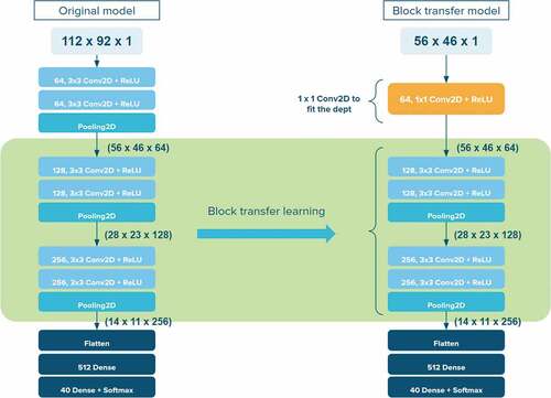
where $f_{\mathrm{c}\mathrm{o}\mathrm{n}\mathrm{v}\left(1\times 1\right)}$ denotes $1\times 1$ convolution. For better acknowledgment, it can be visualized in Figure 5.

Figure 5. An example of block transfer learning. The original model has the input shape $\left(112\times 92\times 1\right)$ with $3$ convolutional blocks. The target model has input shape $\left(56\times 46\times 1\right)$ with $2$ convolutional blocks. The proposed transfer learning method is applied to preserve the knowledge from original model and keep the dedicated input shape of the target model. Then, the identical convolutional layer ($1\times 1$ Conv2D) is added to fit the feature depth.

Experiments

In this section, we experiment to compare and evaluate our proposed method. The experiment includes many preexisting methods for the low-resolution image classification, comparing to our proposed method. At first, we introduce two datasets for the experiments. Besides, the pre-processing images, setting up STF, ATF, and original architectures are described. Finally, we provide the experiment results and some evaluations.

Datasets

We carefully choose two identical datasets for the experiments: ORL (ORL FaceDataset, n.d.) and Cybersoft which are small-scale and medium-scale, respectively. The ORL is public and has widely used in many face recognition problems. The Cybersoft contains images captured in multi-devices with various configurations. Besides, those images are illumination diversity. This dataset is much more complex than the first one. Both two identical datasets capture faces from various perspectives, lightning, and emotions, etc. Table 1 gives detail information about both datasets.

Table 1. Information about ORL and Cybersoft datasets

Dataset name	No. images	No. classes	Original dimensions
ORL	400	40	112 × 92
Cybersoft	800	40	80 × 80

The datasets are applied some conventional pre-processing methods. In particular, all images are rescaled to range $\left[0,1\right]$ and use mean subtraction. The datasets are randomly split into training set and test set with the ratio $7:3$, respectively.

Initialization

Architecture and Scale Transforming Functions

Heuristically, by observation and some experiments, we manually define ${\theta }_s$ and ${\theta }_b$ for both datasets at first, which is ${\theta }_s=\hspace{0.17em}\alpha ,\beta ,s=\left\{\frac{5}{2},\frac{1}{2},0\right\}$ and ${\theta }_b=\hspace{0.17em},\delta ,0b=\left\{1,\frac{1}{2},0\right\}$. Formally,

(7) $\varphi \left(s,{\theta }_s\right)=\frac{5}{2}\cdot s^{\frac{1}{2}}=\frac{5}{2}\sqrt{s}$(7)

(8) $\psi \left(b,{\theta }_b\right)=b^{\frac{1}{2}}=⌈\sqrt{b}⌉$(8)

The initial $r$ where one starts to apply $\varphi \left(\cdot \right)$ and $\psi \left(\cdot \right)$ for ORL and Cybersoft datasets are $r_{\mathrm{O}\mathrm{R}\mathrm{L}}=0.3$, $r_{\mathrm{C}\mathrm{y}\mathrm{b}\mathrm{e}\mathrm{r}\mathrm{s}\mathrm{o}\mathrm{f}\mathrm{t}}=0.4$, respectively. After that, we apply Bayesian Optimization as being proposed to evaluate and compare to the handcrafted hyper-parameters choice.

Original CNN Architectures

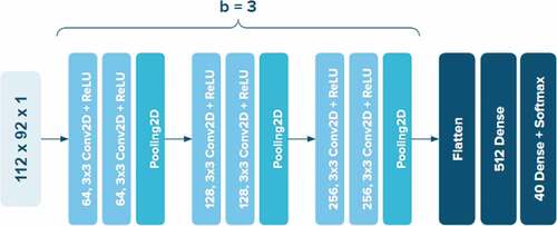
Since VGG-16 (Simonyan and Zisserman 2014) is popular for outperforming most classification tasks, we take their architecture into account with some modification. The first $9$ layers are used instead of the whole network, we also customize the classifier by using only one intermediate fully connected layer with $512$ neurons. Figure 6 illustrates the detail of our modified architecture, which is set up as $3$ blocks ($b=3$) for the feature extraction. This architecture is initialized as the original network for ORL dataset.

Figure 6. The original CNN architecture for training on ORL dataset, which takes first 9 layers from VGG in extraction phase.

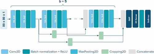
On behalf of the original architecture for the Cybersoft dataset, we take into account a new architecture introduced by Tran et al. called SkippedVGG (Tran et al. 2019). The one recently outperforms in the cap bottle classification task but is light weight compared to some well-known CNN models such as VGG, ResNet, DenseNet, etc. Figure 7 illustrates detail of the architecture. Unlike DenseNet which defines skip connection within each block, SkippedVGG employs it among blocks while preserving sequential stacking in each block. It makes the model more scalable and efficient. In addition, to accelerate the training process and avoid gradient vanishing problem, SkippedVGG takes advantage of batch normalization (Ioffe and Szegedy 2015). We set up $5$ blocks ($b=5$) for the feature extraction.

Figure 7. The original CNN architecture for training on Cybersoft. We follow the concept of SkippedVGG.

In the training phase, all corresponding models including two identical original models and ones produced by $\psi \left(b,{\theta }_b\right)$ are minimized their loss function formulated by cross-entropy. The optimizer is Adam (Kingma and Ba 2014) with initial learning rate $\eta =0.001$. All models are trained in $200$ epochs.

Compared Methods and Metric

To get comprehensive observation, we make comparison with other $9$ methods arising from conventional-interpolation-based and deep-learning-based methods. Our proposed method includes $3$ settings, which is (i) standalone, (ii) combined with block transfer learning and all layers are frozen, and (iii) combined with block transfer learning but all layers are trainable (fine-tuning). All models are evaluated based on classification accuracy metric. As a result, methods used in experiments can be summarized as follow.

• OM – This is the common way when dealing with low resolution images, we keep the same architecture for all CNN models with the input shape that resolutions vary in range scales defined in Algorithm 1. Our purpose is to verify whether this brings better accuracy or not, comparing with dimensions produced by our STF and ATF, i.e $\varphi \left(\cdot \right)$ and $\psi \left(\cdot \right)$.

• NB, BL, BC, BS – These methods are conventional interpolation which up-sample low resolution images back to the original one, such as nearest neighbor, bilinear, bicubic, bspline, respectively, then evaluate on the original model. This is the most popular solution being widely used.

• BL+R, BL+T, BL+RT – To strengthen more quality for bilinear interpolation methods, we integrate it with two popular edge-preserving algorithms Ramponi (Ramponi 1999) and Taguchi (Taguchi and Kimura 2001). In particular, we combine bilinear interpolation with them separately as BL+R, BL+T, respectively, and combine those edge-preserving algorithms together, which is BL+RT.

• SRCNN – We induce SRCNN as deep-learning-based method to compare with the others. The SRCNN architecture is designed that respect to the original one from Dong et al. (Dong et al. 2015). We build models corresponding to the dimensions produced by our $\varphi \left(\cdot \right)$. To speed up the process, we take pre-trained weights from ImageNet (Deng et al. 2009).

• PM – We purely apply our proposed method, which means that all these models are completely trained from scratch.

• PM+TF – Block transfer learning method as being introduced is integrated with our proposed method. Additionally, all layers are frozen except ones in the classifier. This method can be known as feature extraction in transfer learning.

• PM+TF⁺ – The idea is the same as above, but our layers are free to learn during the training. This method is fine-tuning in transfer learning.

Experimental Results

Conventional, Proposed Methods and Block Transfer Learning

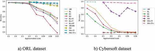
Generally, we conducted two separate experiments, ORL (Orl face dataset, n.d.) and Cybersoft datasets using the initialization as being mentioned. Tables 2 and Table 3 shows the result on ORL. In particular, we compare $3$ proposed methods (PM, PM+TF, PM+TF⁺) with OM, conventional-interpolation-based (NB, BL, BC, BS), those with edge-preserving algorithms (BL+R, BL+T, BL+RT) (Table 2) and deep-learning-based (SRCNN) (Table 3). Meanwhile, the Cybersoft experiment is given in Tables 4 and Table 5, the compared methods are the same as those in ORL excepts BS, BL+R, BL+T, BL+RT and SRCNN. We note that low-resolution inputs that are not satisfy to go through the original architecture are denotes as $-$. Since they are completely flushed out before reaching the output. To illustrate the comparison, we visualized the accuracy results in Figure 8 for ORL and Cybersoft experiments, respectively. The PM+TF shows the bad performance on Cybersoft. This is obvious, since the Cybersoft is much more complex and diverse than the ORL. Only extracting the features from the pre-trained extractor without fine-tuning makes those models almost unlearnable. This problem is overcome by PM+TF⁺, the method gives the highest accuracy comparing with the others.

Table 2. Experiment results on conventional interpolations (ORL Dataset)

Method	$56\times 46$	$44\times 36$	$33\times 27$	$22\times 18$	$11\times 9$	$10\times 8$	$8\times 7$	$6\times 7$	Avg.acc
OM	$0.9833$	$0.9833$	$0.9750$	$0.9583$	$0.8417$	$0.8167$	$-$	$-$	$0.6948$
BL	$0.9750$	$0.9750$	$0.9667$	$0.9667$	$0.8833$	$0.8333$	$0.7667$	$0.6333$	$0.875$
BC	$0.9750$	$0.9667$	$0.9583$	0.9583	$0.8833$	$0.8250$	$0.7417$	$0.6750$	$0.8729$
BS	$0.9750$	$0.9750$	$0.9750$	$0.9750$	$0.7417$	$0.7000$	$0.5300$	$0.3833$	$0.9750$
BL+R	$0.9750$	$0.9750$	$0.9667$	$0.9417$	$0.8333$	$0.7800$	$0.7167$	$0.5667$	$0.5667$
BL+T	$0.9750$	$0.9750$	$0.9750$	$0.9500$	$0.8750$	$0.7917$	$0.7167$	$0.6000$	$0.8573$
BL+RT	$0.9750$	$0.9833$	$0.9667$	$0.9667$	$0.8750$	$0.8333$	$0.7750$	$0.6667$	$0.8802$

Table 3. Experiment results on deep-learning-based interpolations (ORL Dataset)

Method	56×46	$44\times 36$	$33\times 27$	$26\times 24$	$13\times 12$	$9\times 9$	$7\times 7$	$6\times 7$	Avg.acc
SRCNN	$0.9750$	$0.9750$	$0.9750$	$0.9830$	$0.9670$	$0.9500$	$0.9417$	$0.9250$	$0.9615$
PM*	$0.9833$	$0.9833$	$0.9750$	$0.9917$	$0.9833$	$0.9583$	$0.9250$	$0.9083$	$0.9635$
PM+TF*	$0.9833$	$0.9833$	$0.9750$	$0.9833$	$0.9917$	$0.9583$	$0.9667$	$0.9583$	$0.9750$
PM+TF^+*	$0.9833$	$0.9833$	$0.9750$	$0.9833$	$0.9750$	$0.9750$	$0.9667$	$0.9667$	$0.9760$

*Our methods.

Table 4. Experiment results on conventional interpolations (Cybersoft Dataset)

Method	$40\times 40$	$32\times 32$	$24\times 24$	$16\times 16$	$8\times 8$	$7\times 7$	$6\times 6$	Avg.acc
OM	$0.9833$	$0.9792$	$-$	$-$	_	$-$	$-$	$0.2804$
NB	$0.8958$	$0.7542$	$0.4708$	$0.1917$	$0.0833$	$0.0667$	$0.0542$	$0.3595$
BL	$0.6125$	$0.3833$	$0.2042$	$0.0917$	$0.0500$	$0.0417$	$0.0417$	$0.2036$
BC	$0.7833$	$0.6208$	$0.2833$	$0.1208$	$0.0500$	$0.0500$	$0.0500$	$0.2798$

Table 5. Experiment results on deep-learning-based interpolations (Cybersoft Dataset)

Method	$40\times 40$	$32\times 32$	$27\times 27$	$14\times 14$	$9\times 9$	$7\times 7$	$6\times 6$	Avg.acc
PM*	$0.9833$	$0.9792$	$0.9708$	$0.6875$	$0.5542$	$0.8000$	$0.6917$	$0.8095$
PM+TF*	$0.9833$	$0.9792$	$0.0417$	$0.0333$	$0.0500$	$0.0333$	$0.0333$	$0.0383$
PM+TF^+*	$0.9833$	$0.9792$	$0.9708$	$0.9625$	$0.9583$	$0.9417$	$0.9458$	$0.9558$

* ^{Our methods.}

Figure 8. Accuracy of the methods experiment on ORL (left) and Cybersoft (right) dataset.

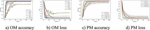
Since OM method acquires training which is similar to our method, we plot the training process of OM and our standalone proposed method (PM). Our purpose is to test the hypothesis that whether our proposed transformation functions perform better than conventional resolution scales or not. As shown in Figure 9, the two first figures show the accuracy and loss in training and validation of OM, the rest figures are the same for PM. It is clear that the OM models significantly drop the accuracy in dimension from scale 0.1. Moreover, they explicitly start over-fitting from the scale 0.2. Our method, on the other hand, tends to outperform where both training and validation accuracy and loss are positively better than OM. Those results complete our hypothesis that the proposed method is more robust.

Figure 9. Training accuracy (solid line) and validation accuracy (dash line) of OM and PM experiments in ORL dataset.

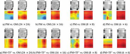
It is worth exploring how CNN models pay attention when dealing with unseen images in various resolutions. By taking advantage of Global Average Pooling (GAP) which is formally introduced in (Lin, Chen, and Yan 2013), we implement Class Activation Map (CAM) to visualize the attention of dedicated models (Zhou et al. 2016). Figure 10 visualizes the CAMs (i.e. heat maps) between the OM and PM, PM+TF⁺ on the Cybersoft dataset. According to the results, those CAMs generated by our methods tend to have better robust attention. In other words, these heat maps higher demarcation contrast of cold and hot areas than those of OM, which seem to be confused where to pay attention in low-resolution image. Additionally, when comparing models between PM and PM+TF⁺, there are significant changes in some cold areas, but still, keep robust to the others. This can be explained as PM+TF⁺ models are succeeded in transferring knowledge from the original trained model.

Figure 10. Class activation map of PM vs. OM methods (top) and PM+TF⁺ vs. OM methods (bottom), the dimensions are $24\times 24$, $16\times 16$, $8\times 8$ and $6\times 6$, respectively.

Bayesian Optimization

Generally, in many kinds of image classification problems, the parameters in ATF and STF functions are variant. It depends on the attribute, distribution, etc. of dataset. Therefore, parameter optimization is taken into account. We would like to integrate Bayesian-based to our proposed method, which is represented by Gaussian Process (Rasmussen and Williams 2005). In this way, it is able to automatically tune the parameters by itself based on the specific kind of dataset. Additionally, we compare with two popular search strategies: random search (Bergstra and Bengio 2012b) and random forest (Liaw and Wiener et al. 2002).

We experiment 3 search strategies on ORL and Cybersoft datasets. Table 6 shows the configuration for both. To simplify the search progress, we predefined some parameters such as learning rate, number of epochs, and number of down-sampled datasets produced by ATF and STF. We also keep the original resolution, model’s architecture and $r$ as well. The searching is limited by 30 iterations for each strategy.

Table 6. The configuration of parameter optimization for ORL and Cybersoft dataset

Dataset	Backbone	Original #blocks	Original resolution	$\mathrm{r}$	Learning rate	#Epochs	# Down-sampled dataset	# Iterations
ORL	VGG	3	$112\times 92$	0.3	0.001	50	5	30
Cybersoft	SkippedVGG	3	$80\times 80$	0.4	0.001	80	5	30

Tables 7 and Table 8 shows the results of ORL and Cybersoft datasets, respectively. The searching provides the optimal $\theta$ that achieves the best average accuracy of down-sampled datasets for each strategy (see Avg.acc column) including the original datasets (ones before $r$) (see Avg.acc+ column). As a result, Bayesian-based (Gaussian Process) is more effective than the others. Impressively, it beats the result of our manual parameter settings for ORL (0.9760) and Cybersoft (0.9558).

Table 7. Parameters optimization by $3$ strategies on ORL Dataset

Dataset	Tuning parameters						Avg.acc	Avg.acc+*
	$\alpha$	$\beta$	${ }_s$	$\gamma$	$\delta$	${ }_b$
Random Search	$2.4518$	$0.7445$	$-0.6443$	$0.7292$	$0.4161$	$-0.3941$	$0.9861$	$0.9819$
Random Forest	$2.8791$	$0.6358$	$0.9751$	$0.79145$	$0.01767$	$0.5754$	$0.9883$	$0.9824$
Gaussian Process	$2.5920$	$0.6063$	$-0.3363$	$0.8643$	$0.5468$	$-0.9028$	$0.9917$	$0.9833$

* ^{Including original datasets.}

Table 8. Parameters optimization by $3$ strategies on Cybersoft Dataset, including Bayesian-based

Dataset	Tuning parameters						Avg.acc	Avg.acc+*
	$\alpha$	$\beta$	${ }_s$	$\gamma$	$\delta$	${ }_b$
Random Search	$1.6585$	$0.5095$	$0.6440$	$0.5286$	$0.9474$	$0.7576$	$0.9708$	$0.9778$
Random Forest	$1.9511$	$0.3082$	$-0.9974$	$0.3710$	$0.8366$	$-0.3952$	$0.8542$	$0.9389$
Gaussian Process	$2.9516$	$0.5417$	$0.5908$	$0.8573$	$0.7309$	$1.0000$	$0.9792$	$0.9805$

*Including original datasets.

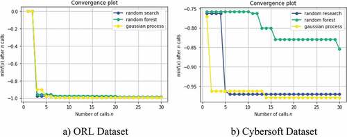
The convergence progress of three search strategies on ORL and Cybersoft are shown in Figure 11. It minimizes the negative accuracy objective function. As a result, the Gaussian Process practically outperforms the random search and random forest. Since it learns from previous sampling experiences, the convergence is also faster the others.

Figure 11. The convergence of 3 search strategies when optimizing on ORL and Cybersoft Dataset.

Conclusion

In this paper, we proposed a new approach to effectively resolve the low-resolution face recognition problem. The experiments show that the method significantly outperforms some other popular ones. Those methods may perform well on high or affordable low resolution. However, they have difficulty handling extremely low dimension and significantly drop in accuracy. Even being enhanced by deep learning method such as SRCNN, those models only show a trivial improvement.

On the other hand, our approach take advantage of both conventional and deep-learning-based methods, and propose transformation functions. These functions learned to produce the optimal resolutions and corresponding CNN model’s architectures varying in a wide range of scales. As a result, our method can deal with any extremely low resolution, yet keep the high accuracy in classification. Moreover, we also enhance the performance and reduce the training time with our block transfer learning strategy. It guides the models to utilize most useful features from the original one without non-trivial tuning, and learning faster than usual. Besides, our method is scalable with any kind of dataset by automated Bayesian optimization that is successfully integrated.

In the future, we will focus on developing automated deep learning model generator and block transfer learning. Our purpose is to completely release the one-stop solution for low-resolution image classification. We hope our proposed method is feasible to apply to many kinds of real-world problems.

Acknowledgments

This work is done by many supports from our colleges in Intelligent Computing and Image Processing laboratory. We would like to thank Trong Vo for special supports and all involved members. Besides, most of the experiments are conducted on the computing system provided by Kyanon Digital LTD. Our special thanks to Tai Huynh, Hang Tran, and all members of the company. We are grateful for all supports and sponsors.

Disclosure Statement

No potential conflict of interest was reported by the author(s).

References

- Bergstra, J., and Y. Bengio. 2012a. Random search for hyper-parameter optimization. Journal of Machine Learning Research 13 (2):281-305.
- Bergstra, J., and Y. Bengio. 2012b. Random search for hyper-parameter optimization. Journal of Machine Learning Research 13 (2):281-305.
- Bulat, A., and G. Tzimiropoulos 2018. Super-fan: Integrated facial landmark localization and super-resolution of real-world low resolution faces in arbitrary poses with gans. Proceedings of the ieee conference on computer vision and pattern recognition, Salt Lake City, UT, USA, 109–1024.
- Chen, J., Z. Chen, Z. Chi, and H. Fu 2014. Emotion recognition in the wild with feature fusion and multiple kernel learning. Proceedings of the 16th international conference onmultimodal interaction, Istanbul Turkey, 508–13.
- Chen, Y., M. Rouhsedaghat, S. You, R. Rao, and -C.-C. J. Kuo 2020. Pixelhop++: A small successive-subspace-learning-based (SSL-based) model for image classification. 2020 IEEE International conference on image processing (ICIP), Abu Dhabi, United Arab Emirates, 3294–98.
- Chen, Y., Y. Tai, X. Liu, C. Shen, and J. Yang 2018. Fsrnet: End-to-end learning face super-resolution with facial priors. Proceedings of the IEEE conference on computer visionand pattern recognition, Salt Lake City, UT, USA, 2492–501.
- Dalal, N., and B. Triggs 2005. Histograms of oriented gradients for human detection. 2005 IEEE computer society conference on computer vision and pattern recognition (cvpr’05), San Diego, CA, USA, vol. 1, 886–93.
- Deng, J., W. Dong, R. Socher, L.-J. Li, K. Li, and L. Fei-Fei 2009. Imagenet: A large-scale hierarchical image database. 2009 ieee conference on computer vision and patternrecognition, Miami, FL, USA, 248–55.
- Dong, C., C. C. Loy, K. He, and X. Tang. 2015. Image super-resolution using deep convo-lutional networks. IEEE Transactions on Pattern Analysis and Machine Intelligence 38 (2):295–307. doi:10.1109/TPAMI.2015.2439281.
- Ge, S., S. Zhao, C. Li, and J. Li. 2018. Low-resolution face recognition in the wild via selective knowledge distillation. IEEE Transactions on Image Processing 28 (4):2051–62. doi:10.1109/TIP.2018.2883743.
- Ge, S., S. Zhao, C. Li, Y. Zhang, and J. Li. 2020. Efficient low-resolution face recognition via bridge distillation. IEEE Transactions on Image Processing 29:6898–908. doi:10.1109/TIP.2020.2995049.
- He, K., X. Zhang, S. Ren, and J. Sun (2016). Deep residual learning for image recognition. Proceedings of the IEEE conference on computer vision and pattern recognition, Las Vegas, NV, USA, 770–78.
- Huang, G., Z. Liu, L. Van Der Maaten, and K. Q. Weinberger (2017). Densely connected convolutional networks. Proceedings of the IEEE conference on computer vision and patternrecognition, Honolulu, HI, USA, 4700–08.
- Ioffe, S., and C. Szegedy (2015). Batch normalization: Accelerating deep network training by reducing internal covariate shift. International conference on machine learning, Lille France, 448–56.
- Kingma, D. P., and J. Ba (2014). Adam: A method for stochastic optimization.arXiv preprintarXiv:1412.6980.
- Koziarski, M., and B. Cyganek. 2018. Impact of low resolution on image recognition with deep neural networks: An experimental study. International Journal of Applied Mathematics andComputer Science 28 (4):735-744.
- Krizhevsky, A., I. Sutskever, and G. E. Hinton. 2012. Imagenet classification with deep convolutional neural networks. Advances in Neural Information Processing Systems 25:1097–105.
- LeCun, Y. A., L. Bottou, G. B. Orr, and K.-R. M ̈uller. 2012. Efficient backprop. In Neural networks: Tricks of the trade, 9–48. Lecture Notes in Computer Science, vol 7700. Springer, Berlin, Heidelberg.
- Li, P., L. Prieto, D. Mery, and P. Flynn (2018). Face recognition in low quality images: A survey.arXiv preprint arXiv:1805.11519.
- Liaw, A., M. Wiener . 2002. Classification and regression by randomforest. R News 2 (3):18–22.
- Lin, M., Q. Chen, and S. Yan (2013). Network in network.arXiv preprint arXiv:1312.4400.
- Lu, Z., X. Jiang, and A. Kot. 2018. Deep coupled Resnet for low-resolution face recognition. IEEE Signal Processing Letters 25 (4):526–30. doi:10.1109/LSP.2018.2810121.
- Minaee, S., and A. Abdolrashidi (2019). Deep iris: Iris recognition using a deep learning approach.arXiv preprint arXiv:1907.09380.
- Ojala, T., M. Pietikainen, and T. Maenpaa. 2002. Multiresolution gray-scale and rotation invariant texture classification with local binary patterns. IEEE Transactions on Pattern analysis and Machine Intelligence 24 (7):971–87. doi:10.1109/TPAMI.2002.1017623.
- Orl face dataset. n.d. http://www.cl.cam.ac.uk/research/dtg/attarchive/facedatabase.html.
- Radford, A., L. Metz, and S. Chintala (2015). Unsupervised representation learning with deep convolutional generative adversarial networks.arXiv preprint arXiv:1511.06434.
- Ramponi, G. 1999. Warped distance for space-variant linear image interpolation. IEEETransactions on Image Processing 8 (5):629–39. doi:10.1109/83.760311.
- Rasmussen, C. E., and C. K. I. Williams. 2005. Gaussian processes for machine learning(adaptive computation and machine learning). The MIT Press.
- Rouhsedaghat, M., Y. Wang, S. Hu, S. You, and -C.-C. J. Kuo. 2021b. Low-resolution face recognition in resource-constrained environments. Pattern Recognition Letters 149:193–99. doi:10.1016/j.patrec.2021.05.009.
- Rouhsedaghat, M., Y. Wang, X. Ge, S. Hu, S. You, and -C.-C. J. Kuo 2021a. Facehop: Alight-weight low-resolution face gender classification method. International conferenceon pattern recognition, Milano, Italy, 169–83.
- Simonyan, K., and A. Zisserman (2014). Very deep convolutional networks for large-scale image recognition arXiv preprint arXiv:1409.1556.
- Snoek, J., H. Larochelle, and R. P. Adams. 2012. Practical Bayesian optimization of machine learning algorithms. Advances in Neural Information Processing Systems 25:3113–21.
- Suykens, J. A., and J. Vandewalle. 1999. Least squares support vector machine classifiers. Neural Processing Letters 9 (3):293–300. doi:10.1023/A:1018628609742.
- Taguchi, A., and T. Kimura. 2001. Edge-preserving interpolation by using the fuzzy technique. Nonlinear Image Processing and Pattern Analysis Xii 4304:98–105.
- Tran, Q. M., L. V. Nguyen, T. Huynh, H. H. Vo, and V. T. Pham 2019. Efficient CNN models for beer bottle cap classification problem. International conference on future data andsecurity engineering, Nha Trang City, Vietnam, 713–21.
- Wang, Z., A. C. Bovik, H. R. Sheikh, and E. P. Simoncelli. 2004. Image quality assessment: From error visibility to structural similarity. IEEE Transactions on Image Processing 13 (4):600–12. doi:10.1109/TIP.2003.819861.
- Weiss, K., T. M. Khoshgoftaar, and D. Wang. 2016. A survey of transfer learning. Journal of Big Data 3 (1):1–40.
- Wold, S., K. Esbensen, and P. Geladi. 1987. Principal component analysis. Chemometrics and Intelligent Laboratory Systems 2 (1–3):37–52. doi:10.1016/0169-7439(87)80084-9.
- Zhou, B., A. Khosla, A. Lapedriza, A. Oliva, and A. Torralba 2016. Learning deep features for discriminative localization. Proceedings of the ieee conference on computer vision andpattern recognition, Las Vegas, NV, USA, 2921–29.
- Zoph, B., and Q. V. Le (2016). Neural architecture search with reinforcement learning.arXiv preprint arXiv:1611.01578.