Artificial Intelligence-Based Image Classification Techniques for Hydrologic Applications

ABSTRACT

Hydrologic modeling is a complex phenomenon dependent on numerous parameters. Since the estimation of parameters is subjected to high uncertainty due to high spatial variation. Therefore, the accuracy of each parameter becomes prime necessary for hydrologic modeling. Gene Expression Programming (GEP) is employed for the first time for Land Use Land Cover (LULC) classification. In the present study, five AI techniques, namely Support Vector Machine (SVM), Adaptive Neuro-Fuzzy Inference System (ANFIS), the M5 Model tree, the multivariate adaptive regression splines (MARS), and Gene Expression Programming (GEP), were studied comparatively for their image classification capability. Comparison criteria adopted for considered AI techniques were errors estimators’ (omission and commission errors) and accuracy estimators’ (overall accuracy and Kappa coefficient). Based on the obtained results, the performance of the GEP technique is found very much comparable with SVM and ANFIS based on overall & Kappa coefficient (>0.85). GEP has a significant advantage over other techniques in producing mathematical functions for the given set of input and output parameters. The present study recommends the use of the GEP technique for LULC image classification.

Introduction

Rain is the primary source of water over the earth. The occurrence of rainfall is seen as a highly uneven activity. Hence, efficient management of watersheds is becoming crucial. The topography of each basin is different; therefore, there is a definite relationship between rainfall and runoff for each basin. Such hydrological modeling involves many parameters and is highly complex too. The impervious nature of the basin plays a vital role in the occurrence of runoff. Estimation of the imperviousness requires the information of classification of land under various usage. This information is nothing but land use and land cover (LULC) classification. There are many ways of classifying, such as physical survey, satellite image, or aerial survey. Physical and aerial surveys are laborious and cumbersome. Satellite image classification is a famous and accurate way of doing classification. The digital satellite image is the approximate 2D representation of the actual situation on the earth’s surface. As a class, identifying and grouping similar spectral property pixels from an image is called image classification. The image of a basin or an area plays a vital role in defining the present assessments and helps future basin planning for better management. Data extracted from such images are the bone of the government’s measures, actions, and rules to be framed. Each basin generates different runoff. The reason is that each basin has a different nature of LULC, which leads to the generation of different imperviousness. The imperviousness is considered in terms of curve number (CN) concerning LULC. This generated curve number concerning image classification is used in hydraulic and hydrological modeling. The image classification based on satellite imagery is challenging due to the high-resolution images and multiple classes depending on the usage. Properly classified imagery is the data set used in the studies related to agriculture, irrigations, water management, town planning, hydrology, watershed management, etc.

Many pattern recognition algorithms and tools are suggested in the literature for image classification (Aksoy et al. 2005; Ferdous et al. 2021; Huang et al. 2012; Zanaty and Afifi 2011). Artificial neural network techniques (ANN) and support vector machines (SVM) are performing well and are popularly adopted techniques for image classification appreciated in medical and other fields (Iqba et al. 2021; Behery, El-Harby, and El-Bakry 2013; Duan, Rajapakse, and Nguyen 2007; Kavzoglu and Colkesen 2009). The images used for hydrological studies are complex and have a wide range of class variability. Hence, the performance of these techniques is still under vigilance, particularly for image classification of a large area. Literature supports that conventional image classification techniques are tiring and prone to high manual errors while training (Kumar et al. 2015; Sunar, Özkan, and Taberner 2004). Many alternative techniques have evolved in the past using pattern recognition techniques to reduce the training efforts and increase the accuracy of classification (Hayri Kesikoglu et al. 2019; Taufik and Ahmad 2016; Rajesh et al. 2014; Behery, El-Harby, and El-Bakry 2013). Prasad, Savithri, and Krishna (2017) found SVM as more promising in image classification over ANN. Similarly, SVM is a better multi-classification algorithm than Bayes discriminant rules, according to Jiang, Lei, and Qin (2016) study. Hayri Kesikoglu et al. (2019) compared maximum likelihood classification (MLC), ANN, and SVM for land use, land cover classification, and change detection. It is concluded that SVM performs better than ANN and MLC (Kumar et al. 2015).

ANFIS is a result of the combined approach of artificial neural networking and fuzzy-logy. Rajesh et al. (2014) compared the ANN-based and ANFIS-based functions to classify the LISS IV image and concluded that ANFIS is better than ANN. Genetic Algorithm (GA) is used to select the features subsets used for training the classification algorithm. Similarly, Şahin, Köse, and Selbaş (2012) also supported that ANFIS is a better approach than ANN. Turkoglu and Avci (2008) made compression between SVM and ANFIS on texture image classification and suggested SVM performing better in terms of training time, and both classifiers perform equally well in classification. A tree-based AI approach is also very famous for the classification of the data. Among them are the decision tree models, Random Forest models, and M5tree models. Among them, the M5 tree is the most advanced and sophisticated model. It is robust and susceptible to the input datasets. Multivariate adaptive regression spline (MARS) is a non-parametric regression analysis technique that robotically models non-linearities relations between variables. These methods are pretty famous in the statistical field of research. However, their performance in multispectral images is still to be exposed. Hence, SVM, ANFIS, M5tree, MARS, and GEP are further considered in this study to analyze their performance for a multiclass and multispectral image from Landsat 8 classification.

Materials and Methods

In this study, Landsat 8 TM image is used for the lower Tapi basin. The basin covers Bardoli, Surat, and some parts of the Bharuch districts in Gujarat, covering an area of around 4,500 Sq.km. It lies between 72°35ʹ3” to 73°35ʹ43” East longitudes and 21°3ʹ10” to 21°39ʹ7” North latitudes. Many researchers have used indices-based classification of the image. The most popular indices are normalized difference vegetation index (NDVI), normalized difference built-up index (NDBI), and modified normalized difference water index (MNDWI) (Li and Chen 2018; Xu 2006). These indices have shown a better separation boundary of each class comparatively for the composite images.

Further, standard training samples as a set of 600 data set points were collected from each class using the high-resolution image of Sentinel 2 A multispectral instrument (MSI) image having 13 spectral bands: 443 nm – 2190 nm. A common platform for execution and examination is used for the performance comparison of the classifier. Figure 1 illustrates the methodology adopted in the present study to test the ability of the classifiers.

Figure 1. The methodology adopted in the present study.

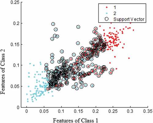
Support Vector Machines (SVM) separates the data optimally into desirable groups by constructing an N-dimensional hyperplane. In SVM, attributes are the predictor variable, and a transformed attribute defines a hyperplane called a feature. SVM model uses a sigmoid Kernel function similar to classic multilayer perceptron neural networks to map the data and classify it into a different space (Yang 2011; Zanaty and Afifi 2011). The procedure for selecting a suitable representation is known as feature selection. Vector is a set of features that describes one class (i.e., a row of predictor variables). Hence, in SVM modeling, an optimal number of hyperplanes are generated that separate clusters of each vector on different sides of the planes. The simplest way to divide two groups according to their attributes is with a straight-line plane. Figure 2 shows the classification of the two classes, that is, water and agriculture using support vectors and hyperplane in two-dimension (2D) space. X- and Y-axis are the hyperplanes of the two classes, and support vectors are catching the values to each class’s domain.

Figure 2. Support vectors and the hyperplane in 2-D space for water and agriculture as class 1 and class 2, respectively.

The Kernel function with SVM’s can define the network’s weights by solving a quadratic programming problem with linear constraints. This approach is an alternative training method to a radial basis function, multilayer perceptron, and polynomial classifiers (Huang, Davis, and Townshend 2002; Kavzoglu and Colkesen 2009). Many Kernel mapping functions, e.g., linear Kernel, polynomial Kernel, exponential Kernel, can be used, probably an infinite number, to define N-hyperplane. Among them, few Kernel functions have worked well for a large variety of operations (Prasad, Savithri, and Krishna 2017). Radial Basis Function (RBF) is the default and recommended Kernel function (Prasad, Savithri, and Krishna 2017; Yang 2011). Using a hyperplane to separate the two feature vectors into two groups is easy to imagine and apply but difficult to classify many feature vectors simultaneously. Among several approaches suggested in the literature, the two most popular approaches are:

(1) “one against many” where every class is separated against all other classes, one by one; and

(2) “one against one” wherein data k number of classes, k(k-1)/2 models were constructed and trained to separate one class from another class.

“One against one” is faster to train is preferred to classify large numbers of classes (Duan, Rajapakse, and Nguyen 2007). In this study, the “one against one” SVM technique is used to classify the image.

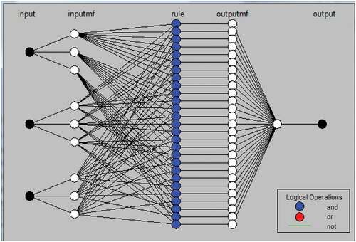
Adaptive Neuro-Fuzzy Inference System (ANFIS)- Fuzzy logic is a widely used principle for decision-making on an incomplete or uncertain dataset. The combined theoretical approach of neural networks and fuzzy is described as the Adaptive neuro-fuzzy inference system (ANFIS). In ANFIS, a fuzzy inference system is attached to the framework of adaptive neural networks. ANFIS has been widely used for image classification in the past by many researchers (Rajesh et al. 2014; Taufik and Ahmad 2016; Madhavan and Kalpana 2017; Cai et al. 2019 and many others). Fuzzy inference follows the fuzzy rule composed of the fuzzification interface, basic rules, database, decision-making element, and defuzzification interface (Taufik and Ahmad 2016). The parameters are selected using a supervised method for fuzzy membership function before training the ANFIS model. This process is essential in achieving the best performance for the fuzzy inference system. For supervised training of ANFIS, the membership functions are determined by providing three inputs based on the output (ground truth information). In this study, three inputs are considered as Normalized difference vegetation index (NDVI), Normalized Difference Water Index (NDWI), and Normalized Difference Built-up Index (NDBI). Input data is based on the ground truth information of vegetation, water, and built-up land. In this study, three inputs were given under three booleans, that is, OR, And, NOT, using three fuzzy if-then rules similar to the Taufik and Ahmad (2016) to classify the five classes. This combination results in the formation of 27 rules (3×3×3) for producing one output. Figure 3 shows the interface of ANFIS used to classify the five classes.

Figure 3. ANFIS model structure adopted in the present study.

M5Tree – M5 tree advanced decision tree-based AI techniques. M5 tree was originally developed by Quinlan (1992). This technique comprises a binary decision tree with linear regression functions on terminal nodes, which can calculate endless numerical attributes. M5 model trees can simulate the phenomena of high dimensionality with many attributes with low computational cost. This is the added advantage of the M5 tree over MARS (Kisi, Shiri, and Demir 2017). The process comprises two different steps. Step 1 is to generate a splitting criterion to initiate the generation of a decision tree. The splitting criterion is based on the standard deviation of the class values of input data. While treating the class values, the standard deviation is considered the attribute that will measure as an error when it reaches the criteria of the node. The class values are tested for each attribute on the node and expected deduction in error. It will produce data split into child and parent nodes with lower and higher standard deviations, respectively. M5 tree among all the possible outcomes of split selects the split which produced maximum expected error reduction. It may result in the formation of a large tree with an overfitting model. In step two, this massive tree is pruned by replacing the subtrees with the linear regression functions. This method helps to generate the splits in parameter space into subspaces and produces a linear regression model.

MARS – Multivariate adaptive regression splines (MARS) was introduced by Friedman in 1991 and is a data-driven nonlinear non-parametric regression analysis. This model is known for its flexible modeling of high-dimensional data. The algorithm aims to produce the small section-wise linear model so that the relationship between predicted and response differs for different predictive variables ranges. Hence the results seem to be continuous series of spline basis functions. These basis functions and parameters are decided using the relationship between input data sets (predicted and response). These spline basis functions give flexibility, continuity, thresholds and allow for bends with a linear relationship between the data sets. This allows the MARS to capture higher-order interactions. Overfitting produced during forwarding – pruning is balanced by backward pruning in the MARS.

Gene Expression Programming (GEP) – GEP is a recently developed computer programming technique among all other techniques. GEP has been widely used for the most sophisticated modeling by researchers (Ferreira 2006; Khan, Azamathulla, and Tufail 2012; Moussa 2013; Najafzadeh, Rezaie Balf, and Rashedi 2016). GEP eliminates some of the limitations of its predecessors as genetic algorithm (GA) and genetic programming (GP) while having combined advantages of both. GEP dealt with both fully-fledged genotype/phenotype systems separately. Hence, GEP performs better in running speed than the old GP system by a factor of 100 to 60,000, promising a more vital ability to resolve the problems (Ferreira 2001). The present study, for the first time, employed a GEP technique for image classification purposes.

In GEP, the process commences random selection of an initial population having peculiar characteristics of the class. This initial population sample helps to generate many pairs of genotype and phenotype comprising an individual chromosome of fixed length for each pair. For potentially practical solutions from all chromosomes, the selection is made based on the fitness value using a fitness proportionate selection operation, generally known as the roulette wheel selection process. Genetic operators replicate the selected chromosome to apply modification, replication, recombination, and transposition to the genomes of the chromosome. This process helps to add the adaptive and evolution nature to the programming. New chromosomes are then brought down to the previous process of selection and modification. The process continues until the required accuracy, and a maximum number of iterations (generations) are achieved (Ferreira 2001, 2002, 2006). The GEP had performed well in predicting bridge pier scour depth compared to regression and ANN models (Mohammadpour 2017). The GEP has a unique approach for selecting and providing compact, explicit solutions by opting for the most optimized solution from all different types of suitable solutions. Hence, this feature supports its suitability, especially for using GEP in getting mathematical expression for computing bridge scours over other AI programming such as ANN (Khan, Azamathulla, and Tufail 2012).

Statistical performances of all three methods SVM, ANFIS, and GEP adopted in the present study were evaluated by considering statistical indices as Commission Error, Omission Error, Producer accuracy, User accuracy, kappa coefficient, and Overall Accuracy. These methods are popularly used and well described in the literature (Hasmadi, Pakhriazad, and Shahrin 2009; Rwanga and Ndambuki 2017).

Results and Discussions

Classification Scheme and Training Samples

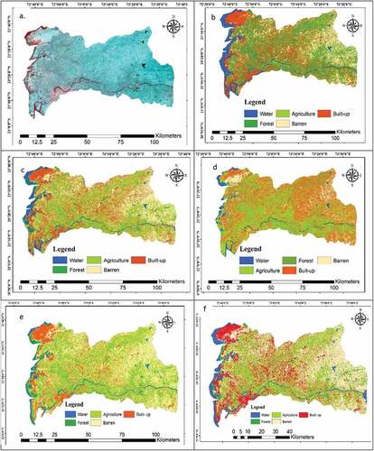
The study area consists of different types of land use and land cover. This study targeted five significant classes: water, forest, agriculture, barren land, and built-up land. In this study, identified training and testing samples were applied uniformly all over the AI techniques during training and testing processes. It will provide a common ground for comparison of their performances. The sampling for the training and testing is prepared with the help of the base map obtained from the Landsat 8 satellite, high-resolution Multispectral Instrument (MSI) image from sentinel-2A of the same period base map from Arch map of high resolution for referencing and cross-checking of sampling. The sampling is prepared in two sets, one set of 600-pixel points per class collecting the information from NDVI, NDWI, and NDBI for training the model and 100-pixel points from each class for testing the output. Figure 4 shows the output result of all AI models during training.

Figure 4. Output results of AI models during training. a. The RGB image of the lower Tapi basin from Landsat 8; b. The SVM model; c. The ANFIS Technique; d. M5Tree; e. Mars; f. The GEP technique.

Errors Estimators

Commission and Omission Error

Commission error indicates the wrongly assigned pixels for a particular class, while omission error indicates the values that belong to a class but were predicted to be in a different class. Commission and omission errors should be zero if the image is correctly classified (Hasmadi, Pakhriazad, and Shahrin 2009). Table 1 indicates commission and omission errors for SVM, ANFIS, M5tree, MARS, and GEP models during training.

Table 1. Commission and omission error for SVM, ANFIS, M5tree, Mars, and GEP models during training (Landsat 8 Satellite image)

Techniques	SVM		ANFIS		M5Tree		MARS		GEP
Classes	Commission error	Omission error	Commission error	Omission error	Commission error	Omission error	Commission error	Omission error	Commission error	Omission error
Water	0.03	0.02	0.01	0.05	0.00	0.05	0.00	0.06	0.01	0.05
Forest	0.23	0.11	0.14	0.11	0.16	0.13	0.27	0.19	0.14	0.10
Agriculture	0.14	0.29	0.14	0.13	0.13	0.15	0.24	0.29	0.11	0.14
Barren land	0.09	0.16	0.12	0.10	0.21	0.10	0.21	0.15	0.14	0.11
Built-up	0.18	0.12	0.10	0.13	0.12	0.19	0.16	0.22	0.11	0.14
Total	0.68	0.70	0.51	0.52	0.62	0.63	0.89	0.91	0.51	0.54

Technique-wise interpretation of results showed that an image classified by the ANFIS method has a minor total omission error compared to others. Class-wise interpretation is more beneficial to understand the probable intermixing of other class pixels in it. The maximum Omission error in MARS is 0.29 for the Agriculture class, maybe due to intermixing of Agriculture class pixels with Forest pixels. The maximum Omission error in ANFIS is 0.13 for the Built-up and Agriculture class. Due to intermixing of built-up class pixels with Barren land pixels and agriculture class with forest class. SVM shows maximum omission error in Agriculture, indicating wrongly assigned pixels of other classes (forest). The high omission error was found to be with MARS and M5 tree Model in all the classes. Water shows a minor omission error compared to others, indicating rightly assigned pixels of the same class. GEP is showing more omission errors for agriculture and built-up classes. Overall performance of the GEP technique is quite comparable with other techniques. A minor error is found for the M5tree technique at the training stage compared with all other classes. It signifies that fewer wrong classified pixels are present in all the classes except agriculture, forest, and built-up.

Similarly, the forest class of MARS has the most significant commission error of about 0.27. It indicates the greater number of wrongly classified pixels in the said class. The image classified by the SVM technique shows that the built-up and forest class contains many wrongly assigned pixels. In general, Agriculture and forest classes are most likely to get mixed. ANFIS and GEP performance for commission error in all classes is comparable low with others in training output. The least total commission error and omission error is found to be with ANFIS at the time of the training model. Now the performances of these techniques are checked with an independent data set. Testing results are shown in Table 2.

Table 2. Commission and omission error for SVM, ANFIS, M5tree, Mars, and GEP models during testing (Landsat 8 Satellite image)

Techniques	SVM		ANFIS		M5Tree		MARS		GEP
Classes	Commission error	Omission error	Commission error	Omission error	Commission error	Omission error	Commission error	Omission error	Commission error	Omission error
Water	0.01	0.02	0.00	0.05	0.01	0.02	0.00	0.03	0	0.02
Forest	0.08	0.08	0.22	0.20	0.09	0.14	0.22	0.17	0.13	0.12
Agriculture	0.06	0.08	0.21	0.21	0.13	0.10	0.17	0.22	0.09	0.13
Barren land	0.07	0.05	0.05	0.01	0.12	0.00	0.16	0.16	0.08	0.01
Built-up	0.05	0.04	0.01	0.03	0.00	0.11	0.15	0.12	0.01	0.03
Total	0.27	0.27	0.49	0.50	0.35	0.37	0.69	0.70	0.31	0.31

The total Commission and omission error for the SVM and GEP technique is the least for the testing data. Commission error and Omission error of ANFIS for Barren land, Built-up, and Water class, whereas Forest and Agriculture show high intermixing of pixels due to indistinguishable features, resulting in high error. High commission error of agriculture and high omission error of forest shows the classification of the forest pixels as agriculture by ANFIS technique and moderate by MARS and M5tree. SVM shows low commission error and omission error on testing data than its training data. SVM technique showed good results while validating with the independent data. GEP technique showed better performance than the other three techniques. From all the above discussion, it can be concluded that classification approaches selected in the present study have shown promising results and can be used for the LULC image classification for Hydrologic applications. However, the individual performance of each technique for each class is different. Therefore, recommending a particular technique as the best technique amongst the five is not possible based only on testing results. Hence, the prediction capability of all techniques is assessed using accuracy estimators (producer accuracy, user accuracy, overall accuracy, and Kappa coefficient) to judge the best AI technique for image classification.

Accuracy Estimators

Producer and User Accuracy

The producer accuracy is the probability of a ground reference being correctly classified. Producer accuracy and omission error are complementary and defined as a ratio of the total number of valid classified pixels of a class to the sum of the column of the class (Jensen 2005). Similarly, user accuracy is the probability that the pixel classified in the map is correctly classified according to the ground data. It is estimated as a ratio of the total number of valid classified pixels in class to the sum of the row of the class (Jensen 2005). The producer and user accuracy nearer to 1 indicates that the applied technique distinguishes the classes accurately, whereas near 0 indicates poor technique’s ability. Both accuracies are estimated at the training and testing stages. The producer and user accuracy results for SVM, ANFIS, M5tree, MARS, and GEP at the training stage are presented in Table 3.

Table 3. Producer and user accuracy for SVM, ANFIS, M5tree, Mars, and GEP at the training stage

Technique	SVM		ANFIS		M5Tree		MARS		GEP
Classes	Producer accuracy	User accuracy	Producer accuracy	User accuracy	Producer accuracy	User accuracy	Producer accuracy	User accuracy	Producer accuracy	User accuracy
Water	0.97	0.98	1.00	0.95	1	0.95	1	0.94	0.99	0.97
Forest	0.77	0.89	0.78	0.89	0.84	0.87	0.73	0.81	0.86	0.92
Agriculture	0.86	0.71	0.79	0.87	0.87	0.85	0.76	0.71	0.89	0.84
Barren land	0.91	0.84	0.95	0.90	0.79	0.9	0.79	0.85	0.86	0.89
Built-up	0.82	0.88	0.99	0.87	0.88	0.81	0.84	0.78	0.89	0.86

Overall performance of SVM, ANFIS, M5tree, MARS, and GEP techniques in terms of producer accuracy is very close to each other. ANFIS, in terms of user accuracy (0.87–0.96), performs the best vis-à-vis the other two methods based on its ability to classify pixels of a particular class. The method’s performance depends significantly on how accurately it prevents or separates the intermixing pixels of other classes. There are higher chances of pixel intermixing with similar spectral reflectance priorities (e.g., forest and agriculture, barren, and built-up land). User accuracy of SVM (0.88–0.98) represents the best ability vis-à-vis the other four methods to separate the intermixed pixels of other classes in a particular class. It is also observed that the particular method performs well for a particular class, either indeed assigning pixels or separating intermixing pixels for that particular class. As SVM classifies the water class more accurately, the other four classes are less accurately distinguished. SVM and GEP techniques showed comparable performance during the training stage. M5tree and MARS scores less user accuracy than other AI techniques.

Further, to check the performances of the selected techniques with independent data, again, the same accuracy indicators are used, and results are shown in Table 4. Inconsistency in the result is observed at the testing stage. The SVM and GEP have scored better producer and user accuracy than other AI techniques. Therefore, ranking techniques become difficult based on the testing results.

Table 4. Producer and user accuracy for SVM, ANFIS, M5tree, Mars, and GEP at the testing stage

Method	SVM		ANFIS		M5Tree		MARS		GEP
Classes	Producer accuracy	User accuracy	Producer accuracy	User accuracy	Producer accuracy	User accuracy	Producer accuracy	User accuracy	Producer accuracy	User accuracy
Water	0.99	0.98	1.00	0.95	0.99	0.98	1	0.97	1.00	0.99
Forest	0.92	0.92	0.78	0.80	0.91	0.86	0.78	0.83	0.87	0.88
Agriculture	0.94	0.92	0.79	0.79	0.87	0.9	0.83	0.78	0.92	0.87
Barren land	0.93	0.95	0.95	0.99	0.88	1	0.84	0.84	0.93	0.99
Built-up land	0.95	0.96	0.99	0.97	1	0.89	0.85	0.88	0.99	0.97

Overall Accuracy and Kappa Coefficient

Based on overall accuracy and kappa coefficient analysis, all three techniques are examined for performance and ranking. Overall accuracy is defined as the probability of classifying a pixel correctly to the actual class. It is measured by the sum of truly classified pixels and wrongly classified pixels to the total number of pixels tested in all. It represents the percentage of correctly classified pixels in an image.

Cohen’s kappa coefficient (κ) gives the statistical measure of the reliability for qualitative classification among the classes. Kappa coefficient is described by Eq. 1(1) $K=\frac{\left(Totalnumberofcorrectlyplacedpixel\right)-\left(totaloftheproductofExpectedFrequency\right)}{\left(Totalnumberofthepixelsinallclass\right)-\left(totaloftheproductofExpectedFrequency\right)}$(1) .

(1) $K=\frac{\left(Totalnumberofcorrectlyplacedpixel\right)-\left(totaloftheproductofExpectedFrequency\right)}{\left(Totalnumberofthepixelsinallclass\right)-\left(totaloftheproductofExpectedFrequency\right)}$(1)

It is represented as a “$\hspace{0.17em}$κ“; which estimates how well pixels can be precisely classified. This statistic measures the degree of agreement or disagreement between a classified pixel and its linked reference pixel. The value of $\hspace{0.17em}$ “κ“ is more significant than 0.75, it depicts strong agreement, values fall between 0.65 and 0.7 is considered moderate agreement, and the value falls less than 0.65, which signifies poor agreement (Jensen 2005). Obtained results for kappa Coefficient and overall accuracy for the SVM, ANFIS, and GEP techniques are presented in Table 5.

Table 5. Kappa coefficient and overall accuracy for SVM, ANFIS, M5tree, Mars, and GEP method (During training and testing stage)

Method	Training		Testing
	kappa Coefficient	Overall Accuracy	kappa Coefficient	Overall Accuracy
SVM	0.83	0.86	0.93	0.95
ANFIS	0.87	0.90	0.88	0.90
M5Tree	0.84	0.87	0.91	0.92
MARS	0.77	0.82	0.83	0.86
GEP	0.87	0.90	0.93	0.94

All the methods have accuracy in terms of kappa coefficient and overall accuracy greater than 0.85 during training and testing stages. All the techniques have shown better performance in testing than in training. However, SVM and GEP are showing the best performance at the testing stage, followed by M5tree ANFIS and MARS. Hence, all techniques are found suitable for image classification.

Conclusions

For a hydrologic modeler, an accurately classified image is a very crucial input parameter. Artificial intelligence techniques are replacing traditional image classification techniques due to their ability to categorize pixels accurately. Prime input to the Curve Number (CN) based stream discharge estimation technique is the soil map and LULC image. The accuracy of hydrologic output would greatly depend on how accurate a LULC map is parallel to the other parameters. This study highlights the AI techniques available for the LULC classification of satellite data into five classes (Water, Forest, Agriculture, Barren, Built-up) used for the hydrological studies. This study is limited to comparing the performance of the basic AI techniques SVM ANFIS M5 tree MARS and GEP. A state-of-the-art GEP is first time introduced in the present study for its application in image classification. GEP has a significant advantage over other techniques in producing mathematical functions for the given set of input and output parameters. GEP model when trained for the hydrologic basin irrespective of season, then that model can be used for the next few years without using any high computational power or large training algorithm. In the present study, GEP performance is found very much comparable with other AI techniques. GEP has a dynamic nature of learning with a high potential to produce better-classified images.

The SVM method attains a better LULC classification power during the testing phase. It is a non-parametric classifier that finds a linear/nonlinear vector to separate input instances. SVMs require substantially more training data than k-nearest neighbors’ algorithms (kNN) but less than neural networks (to get a decent performance). The SVM model using a sigmoid kernel function is equivalent to a two-layer, perceptron neural network. The complexity of neural networks is well thought under the SVM; hence, SVM naturally performs well.

The results presented in the present study are highly encouraging for using AI techniques for image classification. It is concluded that SVM, GEP, M5tree, ANFIS, and MARS techniques are promising in modeling LULC, and this study provides a valuable reference for researchers and engineers who apply AI techniques for LULC modeling for Hydrologic applications.

Disclosure Statement

No potential conflict of interest was reported by the author(s).

Correction Statement

This article has been republished with minor changes. These changes do not impact the academic content of the article.

References

- Aksoy, S., K. Koperski, C. Tusk, G. Marchisio, and J. C. Tilton. 2005. Learning Bayesian classifiers for scene classification with a visual grammar. IEEE Transactions on Geoscience and Remote Sensing 43 (3):581–1156. doi:10.1109/TGRS.2004.839547.
- Behery, G. M., A. A. El-Harby, and M. Y. El-Bakry. 2013. Anfis and neural networks systems for multiplicity distributions in proton-proton interactions. Applied Artificial Intelligence 27 (4):304–22. doi:10.1080/08839514.2013.774212.
- Cai, G., H. Ren, L. Yang, N. Zhang, M. Du, and C. Wu. 2019. Detailed urban land use land cover classification at the metropolitan scale using a three-layer classification scheme. Sensors 19 (14):3120–44. doi:10.3390/s19143120.
- Duan, K. B., J. C. Rajapakse, and M. N. Nguyen (2007). One-versus-one and one-versus-all multiclass SVM-RFE for gene selection in cancer classification. In European Conference on Evolutionary Computation, Machine Learning and Data Mining in Bioinformatics. Springer, Berlin, Heidelberg. 47–56
- Ferdous, H., T. Siraj, S. J. Setu, M. M. Anwar, and M. A. Rahman (2021). Machine learning approach towards satellite image classification. In Proceedings of International Conference on Trends in Computational and Cognitive Engineering (pp. 627–37). Springer, Singapore.
- Ferreira, C. 2001. Gene expression programming: A new adaptive algorithm for solving problems. Complex Syst 13 (2):87–129.
- Ferreira, C. 2002. Mutation, transposition, and recombination: An analysis of the evolutionary dynamics. Joint Conference on Information Sciences 6 (4):614–17.
- Ferreira, C. 2006. gene expression programming, studies in computational intelligence. Berlin: Springer-Verlag.
- Friedman, J. H. 1991. Multivariate adaptive regression splines. The Annals of Statistics 19 (1):1–67.
- Hasmadi, M., H. Z. Pakhriazad, and M. F. Shahrin. 2009. Evaluating supervised and unsupervised techniques for land cover mapping using remote sensing data. Geografia: Malaysian Journal of Society and Space 5 (1):1–10.
- Hayri Kesikoglu, M., U. Haluk Atasever, F. Dadaser-Celik, and C. Ozkan. 2019. Performance of ANN, SVM, and MLH techniques for land use/cover change detection at Sultan Marshes wetland, Turkey. Water Science and Technology 80 (3):466–77. doi:10.2166/wst.2019.290.
- Huang, C., L. S. Davis, and J. R. G. Townshend. 2002. An assessment of support vector machines for land cover classification. Int J Remote Sens 23 (4):725–49. doi:10.1080/01431160110040323.
- Huang, G.-B., H. Zhou, X. Ding, and R. Zhang. 2012. Extreme learning machine for regression and multiclass classification. IEEE Transactions on Systems, Man, and Cybernetics. Part B, Cybernetics 42 (2):513–29. doi:10.1109/TSMCB.2011.2168604.
- Iqbal, M. S., Ahmad, I., Bin, L., Khan, S., & Rodrigues, J. J. 2021. Deep learning recognition of diseased and normal cell representation. Transactions on Emerging Telecommunications Technologies 32 (7):e4017.
- Jensen, J. R. 2005. Digital image processing: A remote sensing perspective. Upper Saddle River, NJ: sPrentice Hall.
- Jiang, T., P. Lei, and Q. Qin. 2016. An application of SVM-based classification in landslide stability. Intelligent Automation & Soft Computing 22 (2):267–71. doi:10.1080/10798587.2015.1095480.
- Kavzoglu, T., and I. Colkesen. 2009. A Kernel functions analysis for support vector machines for land cover classification. Int J Appl Earth Obs Geoinfr 11 (5):352–59. doi:10.1016/j.jag.2009.06.002.
- Khan, M., H. M. Azamathulla, and M. Tufail. 2012. Gene-expression programming to predict pier scour depth using laboratory data. Journal of Hydroinformatics 14 (3):628–45. doi:10.2166/hydro.2011.008.
- Kisi, O., J. Shiri, and V. Demir. 2017. Hydrological time series forecasting using three different heuristic regression techniques. In Handbook of Neural Computation, ed. Pijush Samui, Sanjiban Sekhar, Valentina E. Balas, Academic Press, 45–65.
- Kumar, P., D. K. Gupta, V. N. Mishra, and R. Prasad. 2015. Comparison of support vector machine, artificial neural network, and spectral angle mapper algorithms for crop classification using LISS IV data. International Journal of Remote Sensing 36 (6):1604–17. doi:10.1080/2150704X.2015.1019015.
- Li, K., and Y. Chen. 2018. A genetic algorithm-based urban cluster automatic threshold method by combining VIIRS DNB, NDVI, and NDBI to monitor urbanization. Remote Sensing 10 (2):277–98. doi:10.3390/rs10020277.
- Madhavan, E., and S. Kalpana. 2017. Building Identification in Satellite Images Using ANFIS Classifier. Asian Journal of Applied Science and Technology (AJAST) 1:283–85.
- Mohammadpour, R. 2017. Prediction of local scour around complex piers using GEP and M5-Tree. Arabian Journal of Geosciences 10 (18):416–27. doi:10.1007/s12517-017-3203-x.
- Moussa, Y. A. M. 2013. Modelling of local scour depth downstream hydraulic structures in trapezoidal channel using GEP and ANNs. Ain Shams Engineering Journal 4 (4):717–22. doi:10.1016/j.asej.2013.04.005.
- Najafzadeh, M., M. Rezaie Balf, and E. Rashedi. 2016. Prediction of maximum scours depth around piers with debris accumulation using EPR, MT, and GEP models. Journal of. Hydroinformatics 18 (5):867–84. doi:10.2166/hydro.2016.212.
- Prasad, S. V. S., T. S. Savithri, and I. V. M. Krishna. 2017. Comparison of accuracy measures for RS image classification using SVM and ANN classifiers. International Journal of Electrical and Computer Engineering 7 (3):1180–87.
- Quinlan, J. R. (1992). Learning with continuous classes. Proc., 5th Australian Joint Conf. on Artificial Intelligence, Adams & Sterling, eds., World Scientific, Singapore, 343–48. https://doi.org/10.1142/1897
- Rajesh, S., Arivazhagan, S., Moses, K. P., & Abisekaraj, R. 2014. ANFIS based land cover/land use mapping of LISS IV imagery using optimized wavelet packet features. Journal of the Indian Society of Remote Sensing, 42(2), 267–277.
- Rwanga, S. S., and J. M. Ndambuki. 2017. Accuracy assessment of land use/land cover classification using remote sensing and GIS. International Journal of Geosciences 8 (4):611–15. doi:10.4236/ijg.2017.84033.
- Şahin, A. Ş., İ. İ. Köse, and R. Selbaş. 2012. Comparative analysis of neural network and neuro-fuzzy system for thermodynamic properties of refrigerants. Applied Artificial Intelligence 26 (7):662–72. doi:10.1080/08839514.2012.701427.
- Sunar, E. F., C. Özkan, and M. Taberner. 2004. Comparison of maximum likelihood classification method with supervised artificial neural network algorithms for land use activities. International Journal of Remote Sensing 25 (9):1733–48. doi:10.1080/0143116031000150077.
- Taufik, A., and S. S. S. Ahmad. 2016. Land cover classification of Landsat 8 satellite data based on Fuzzy Logic approach. IOP Conference Series: Earth and Environmental Science 37 (1):12062–70. doi:10.1088/1755-1315/37/1/012062.
- Turkoglu, I., and E. Avci. 2008. Comparison of wavelet-SVM and wavelet-adaptive network-based fuzzy inference system for texture classification. Digital Signal Processing: A Review Journal 18 (1):15–24. doi:10.1016/j.dsp.2007.09.011.
- Xu, H. 2006. Modification of normalised difference water index (NDWI) to enhance open water features in remotely sensed imagery. International Journal of Remote Sensing 27 (14):3025–33. doi:10.1080/01431160600589179.
- Yang, X. 2011. Parameterizing support vector machines for land cover classification. Photogramm Eng Remote Sens 77 (1):27–37. doi:10.14358/PERS.77.1.27.
- Zanaty, E. A., and A. Afifi. 2011. Support vector machines (SVMs) with universal kernels. Applied Artificial Intelligence 25 (7):575–89. doi:10.1080/08839514.2011.595280.