A Hybrid Improved Whale Optimization Algorithm with Support Vector Machine for Short-Term Photovoltaic Power Prediction

ABSTRACT

Presently, the grid-connected scale from photovoltaic (PV) system is getting higher among renewable power generations. However, the PV output power can be affected by different meteorological conditions due to PV randomness and volatility. Accordingly, reasonable generation plans can be well arranged using accurate PV power prediction among various types of energy sources, thus reducing the effect of PV system on the grid. To resolve this problem, a PV output power prediction model, namely IMWOASVM, is proposed based on the combination of improved whale optimization algorithm (IMWOA) and support vector machine (SVM). The IMWOA is used to optimize the kernel function parameter and penalty coefficient in SVM. The optimal parameter and coefficient values can then be input to SVM for enhancing the PV prediction. The performance results verify that the coefficient of determination using the IMWOA model can reach beyond 99% in both sunny and cloudy days. Simultaneously, the mean absolute errors on sunny and cloudy days are 0.0251 and 0.0705, respectively. The root mean square errors in sunny and cloudy days are 2.17% and 1.03%, respectively. The results confirm that the proposed model effectively increases the accuracy of the PV output power prediction and is superior to existing methods.

Introduction

With increasing global energy demand, the utilization and development of renewable energy have been becoming more and more important in the power industry (Yu et al. 2019). Solar is one of the most crucial renewable energy resources (Wang, Qi, and Liu 2019). Therefore, the development of PV power technology is considered as an effective solution to alleviate the world energy crisis (Carvajal-Romo et al. 2019). In 2016, the annual photovoltaic (PV) power generation has exceeded wind power, and the installed capacity of global PV system was 48% higher compared with 2015 (Gurung, Naetiladdanon, and Sangswang 2019). However, PV power generation is fluctuating and intermittent at all times due to the uncertainty of light intensity and other meteorological conditions (Liu et al. 2018). In addition, some factors like weather, season and others post more difficulty for PV power dispatching in grid (Gandoman, Raeisi, and Ahmadi 2016; VanDeventer et al. 2019). To address this issue, the prediction of PV power generation can provide important information for reasonable grid power planning and economic dispatching (Chai et al. 2019; Han et al. 2019; Liu, Zhan, and Bai 2019; Wang et al. 2018a).

The prediction methods for PV output power can be classified as follows: long- and medium-term forecast is used for the maintenance and operation management of photovoltaic power stations in weekly units. Short-term forecast is used to arrange reasonable daily power generation in hourly or daily units (Ni et al. 2017). Ultra-short-term forecasting is used for real-time dispatching of power grids in minutes or 1 hour (Monfared et al. 2019). In the economic dispatching of power grid, He et al. (2019) suggested that the short-term prediction played a decisive role, which directly influenced the security and stability of the system operation. Semero, Zheng, and Zhang (2018) also pointed out that the planning based on short-term prediction in the PV system can promise the reliable and economical of power supply. Alternatively, the forecast methods of PV output power are classified into direct and indirect ones. Indirect method is to estimate the output power according to the predicted variables. Due to the complex and changeable weather conditions, the current prediction accuracy is still insufficient (Pierro et al. 2017). The direct method is to directly take the historical data as input variables to predict the power output (Gao et al. 2019). It usually used the linear forecast model with time series, nonlinear model and mixed model of the two. Autoregressive moving average (ARMA) model and autoregressive (AR) model belong to time-series model (Bae et al. 2019). Among the nonlinear prediction methods, there are increasing application cases using such as extreme learning machine (ELM), support vector machine (SVM) and back propagation neural network (BP), aiming at minimum prediction error (Lin et al. 2018; Rana, Koprinska, and Agelidis 2016). Li et al. (2016) used hidden Markov and support vector machine regression model to predict short-term PV generation from solar radiation intensity. Li et al. (2019) applied the SVM model combined with the hybrid improved multi-verse optimizer for the short-term PV power output prediction. Wang, Qi, and Liu (2019) revealed that the photovoltaic power prediction is of great help to the stable operation of photovoltaic system.

To enhance the forecast ability, the direct prediction method is selected to predict the PV output power in this study. The support vector machine model is used as the prediction model, and the improved whale optimization algorithm (IWOA) is developed to search for the optimal parameter combination in the support vector machine model. The article consists of six major sections. Section 2 gives literature reviews on photovoltaic power generation prediction methods. Section 3 introduces the construction of the integrated prediction model, including the improved whale optimization algorithm and support vector machine model. The results and analysis of photovoltaic power generation prediction are provided in Section 4. The discussion is presented in Section 5. The conclusions are made in Section 6.

Literature Review

Wang et al. (2018b) used ARMA, BP and SVM model to predict PV power generation. The results showed that the proposed method could effectively increase the prediction accuracy. Xie et al. (2018) proposed a short-term hybrid forecast model, which mixed deep confidence network (DBN) and variational mode decomposition (VMD) in ARMA, which could better regulate the operation of power system. Raza, Nadarajah, and Ekanayake (2017) used a hybrid model, including wavelet transform (WT), ARMA, radial basis function (RBF) and neural network to predict a short-term PV power. However, it may cause a large deviation in the model due to the lack of nonlinear mechanism involved.

To enhance the precision of PV power generation forecast, Al-Dahidi et al. (2019) proposed an artificial neural network model that combined 10 different learning algorithms and 23 different training data sets. However, the proposed model was complex with limitations in its application scenarios. Hua et al. (2019) reported a long-term and short-term memory back propagation (LSTM-BP) method in the power generation forecast. Unfortunately, the training speed of this algorithm was slow, where all network parameters needed to be updated during each training process.

Al-Dahidi et al. (2018) developed an extreme learning machine (ELM) model to predict PV power generation in a 264 kWp PV system. The simulation results revealed that the forecast with ELM model was more accurate than the BP neural network model. Cheng, Liu, and Zhang (2019) proposed an optimization model to enhance the ELM model parameters using the genetic algorithm (GA), and Gaussian mixture model (GMM) was used to correct the forecasted values in PV power generation. Liu et al. (2020) introduced a chicken flock optimizer to optimize the ELM parameters for forecasting PV power under various meteorological conditions. The results showed that a better forecast precision was achieved.

Mojumder et al. (2016) simplified the complex mathematical problems in PV power prediction using SVM model with the combination of wavelet, radial basis function and firefly algorithm. To effectively solve the security problems in grid-connected PV system, Eseye, Zhang, and Zheng (2018) proposed a particle swarm optimization SVM (PSOSVM) model, showing better short-term PV power generation forecast than the SVM models. van der Meer et al. (2018) combined genetic algorithm with SVM model to achieve more accurate prediction than SVM models. Yang, Zhu, and Peng (2020) applied a gray correlation theory to find the main factors that may affect the consumption of clean energy. The results showed that the proposed model has a good forecast performance.

Currently, some research has been working on the improvement of whale optimization algorithm (WOA). For example, Xiong, Hu, and Guo (2021) improved the WOA convergence speed by introducing a nonlinear adjustment scheme. It was then used to optimize the gray seasonal variation index model to achieve high prediction accuracy with fast speed. On initialization of the whale population, Gao et al. (2022) applied random method and chaotic sequence method to generate two initialization populations, which enhanced the diversity of individuals. Two different convergence strategies were also introduced for boosting the search ability of algorithm. It was then used to optimize the ELM model for better prediction accuracy with less time required. Liu et al. (2021a) integrated SVM into the WOA. The initial population became diverse and the optimization ability was thus enhanced. The improved algorithm was then used to optimize the SVM model to improve the prediction accuracy, but the complex nonlinear relationship behind the data was not deeply considered.

Construction of Prediction Model

Principle and Improvement of WOA

WOA is based on the unique predation strategy from humpback whales. In the optimization process, three stages are regarded as the main parts of search and optimization (Mirjalili and Lewis 2016a; Simhadri and Mohanty 2019; Yuan et al. 2018).

1. Foraging encirclement stage

When a whale is close to the prey location, the whale group will immediately work together to approach toward the target for rounding up. The whale position updating process is shown below.

(1) $x_{t+1}=x_t^{\ast }-AD$(1)

(2) $D=\left|C{x}_t^{\ast }-x_t\right|$(2)

where $x_t$ is the position of the individual of the whale group. $x_t^{\ast }$ is the position of the optimal individual in the whale group. $x_{t+1}$ is the individual position of the whale group after update. $D$ represents the distance between the whale and the optimal individual. $A$ and $C$ are the coefficients, defined as follows.

(3) $A=2a{n}_1-C$(3)

(4) $C=2n_2$(4)

where $n_1$ and $n_2$ are randomly chosen between the range 0 and 1. The value of $a$ is located between 0 and 2, where it decreases with the increasing iteration in a linear downward trend.

1. Bubble predation stage

The bubble predation behavior of humpback whales includes two processes: shrink encirclement and spiral rise. Shrinking encirclement means that the individual closest to the prey is selected as the best search agent in the whale population, and other whales will move closer to the currently selected whale individual. Each whale updates its position according to the current optimal position of the population, and adjusting the coefficient values of $A$ and $C$ can control the whale to search near its prey.

Whales can perform spiral contraction encirclement behavior according to the value of $a$. The spiral rising process is used to simulate the whale spiral motion, and the whale position updating equation is shown below.

(5) $D^{\prime }=\left|x_t^{\ast }-x_t\right|$(5)

(6) $x_{t+1}=x_t^{\ast }+D\prime e^{bl}cos(2\pi l)$(6)

where $D^{\prime }$ is the distance between the prey and whale, $l$ is randomly chosen between the range −1 and 1, and $b$ is a constant to represent the shape of the helix.

To simulate the simultaneous occurrence in contraction encirclement and spiral rise, a mathematical model for whale position updating is constructed, as shown below:

(7) $x_{t+1}=\left\{\begin{array}{c}{x}_t^{\ast }-AD\\ x_t^{\ast }+D\prime e^{bl}cos(2\pi l)\end{array}\right.\begin{array}{c}\hspace{0.17em}\\ \hspace{0.17em}\end{array}\begin{array}{c}p<0.5\\ p\ge 0.5\end{array}$(7)

The value of $p$ is randomly chosen and uniformly distributed between 0 and 1. According to the value of $p$, the whale chooses spiral model or contraction encirclement to change its position during the optimization process. When $p$ is less than 0.5, the whale will perform the contraction encirclement process. If $p$ is greater than 0.5, the whale will move in a spiral. Note that $p$ is a uniform distribution between [0, 1], and the probability of choosing both modes are 50%.

1. Food search stage

The whale food search behavior is realized by changing the value of $A$. In Equation (3)(3) $A=2a{n}_1-C$(3) , $A$ is a random number between [-$a$, $a$]. When $\left|A\right|$ is greater than 1, a search agent is stochastically chosen to change the position of other whales for enhancing the WOA exploration capability. Consequently, the whale can accomplish the global search by approaching the position of the whale that has been randomly selected. The whale position $x{\hspace{0.17em}}_t$ is updated to $x{\hspace{0.17em}}_{t+1}$ as follows.

(8) $D_{rand}=\left|C{x}_{rand}-x_t\right|$(8)

(9) $x_{t+1}=x_{rand}-A{D}_{rand}$(9)

where $x_{rand}$ is the position of a randomly selected whale. $D_{rand}$ represents the distance between the whale and the randomly selected individual.

The WOA starts with a random position, and the search agent changes its position from every iteration according to the optimal individual currently available or the randomly selected search agent. When $\left|A\right|>1$, select the stochastic search agent; when $\left|A\right|<1$, select the optimal position to update the position of the search agent. The value of $p$ can determine whether WOA will carry out contraction encirclement or spiral motion. Finally, the WOA algorithm process stops once the specified iteration number is reached.

When WOA is applied to high-dimensional problems, it may only obtain the local optimal solution, which leads to the deterioration or even failure of the optimization effect. To prevent the WOA from being trapped into a locally optimal solution, an adaptive factor is introduced, and the position update Equation (1)(1) $x_{t+1}=x_t^{\ast }-AD$(1) is updated. The updated equation is as follows:

(10) $x_{t+1}=Q{x}_t^{\ast }-AD$(10)

(11) $Q=1+sin\frac{\pi (2t_{max}+t)}{2t_{max}}$(11)

$Q$ represents the adaptive factor. As the number of iterations increases, the value of $Q$ will gradually decrease from 1 to 0. The improved position update equation can enable whales to conduct local optimization while approaching prey, thus improving the local search capability of WOA.

To further promote the WOA global search capability, the mutation operator is introduced. The improved equation is expressed as follows..

(12) $x_{t+1}=x_{rand}-A\cdot Cauchy(t)$(12)

where $Cauchy(t)$ denotes a random variable that obeys the Cauchy distribution. It is used to increase the search randomness in the whale optimization algorithm, and thus the global search capability can be enhanced.

Performance Test of Improved WOA

In this study, eight test functions are selected to test the convergence ability of the IMWOA, as shown in Table 1 (Li et al. 2021a; Liu et al. 2021b). The IMWOA, MVO, Ant Lion Optimizer (ALO), WOA, Grasshopper Optimization Algorithm (GOA), particle swarm optimization (PSO) and Seagull optimization algorithm (SOA) are tested and compared (Dhiman and Kumar 2019; Mirjalili 2015; Mirjalili, Mirjalili, and Hatamlou 2016b; Shahrzad et al. 2017; Zhang, Wang, and Lu 2022). Under the same conditions, the populations are set as 30, the iterations are set as 500, the dimensions are set as 30, and the other parameters are default values. Each model is tested for 30 times, and the maximum, minimum and average values of each test are listed in Table 1, where the bound denotes the value range of $x_i$ and $x_j$, and $F_{min}$ is the minimum value for which the function converges (Mirjalili and Lewis 2016). The convergence values in various test functions are shown in Table 2.

Table 1. Test functions

Function	Dim	Bound	$F_{min}$
$F_1(x)=\sum _{i=1}^n{x_i}^2$	30	[−100,100]	0
$F_2(x)=\sum _{i=1}^n\left|x_i\right|+\prod _{i=1}^n\left|x_i\right|$	30	[−10,10]	0
$F_3(x)=\sum _{i=1}^n(\sum _{j-1}^i{x}_j{)}^2$	30	[−100,100]	0
$F_4(x)=-20exp(-0.2\sqrt{\frac{1}{n}{\sum }_{i=1}^n{x}_i^2})-exp(\frac{1}{n}{\sum }_{i=1}^{n}cos(2\pi x_i))+20+e$	30	[−32,32]	0
$F_5(x)=\frac{1}{4000}{\sum }_{i=1}^n{x}_i^2-{\mathrm{\Pi }}_{i=1}^{n}cos(\frac{x_i}{\sqrt{i}})+1$	30	[−600,600]	0
$F_6(x)=\frac{\pi }{n}\{10sin(\pi y_1)+{\sum }_{i=1}^{n-1}{(y_i-1)}^2[1+10{sin}^2(\pi y_{i+1})]+{(y_n-1)}^2\}+{\sum }_{i=1}^{n}u(x_i,10,100,4)$	30	[−50,50]	0
$F_7(x)={\sum }_i^{n-1}[100{(x_{i+1}-x_i^2)}^2+{(x_i-1)}^2)]$	30	[−30,30]	0
$F_8(x)={\sum }_i^{n}i{x}_i^4+randm[0,1)$	30	[1.28,-1.28]	0

Table 2. Test convergence values

Test functions	Algorithms	Max	Average	Min
$F_1$	WOA	3.0370e-72	1.6045e-73	2.5790e-87
	IMWOA	6.9774e-196	2.3276e-197	1.5097e-219
	ALO	7.5689e-09	4.1167e-09	1.4894e-09
	MVO	0.0203	0.0087	0.0036
	GOA	7.1766e-08	1.8157e-08	2.3434e-09
	PSO	1.0343	0.1779	0.0493
	SOA	5.3009e-11	4.9588e-12	1.3316e-13
$F_2$	WOA	2.4396e-50	1.7536e-51	7.8237e-58
	IMWOA	2.2833e-107	1.2818e-108	2.1301e-118
	ALO	2.5565	0.3928	1.1619e-05
	MVO	0.0443	0.0279	0.0152
	GOA	8.5381	2.2464	4.4077e-04
	PSO	2.7152	1.4421	0.6817
	SOA	1.0053e-07	1.9781e-08	2.8402e-09
$F_3$	WOA	7.0896e+04	4.5925e+04	2.2949e+04
	IMWOA	5.1658e-153	1.7220e-154	1.8131e-188
	ALO	0.0342	0.0027	1.3541e-05
	MVO	0.1101	0.0411	0.0047
	GOA	0.1031	0.0034	1.2066e-09
	PSO	105.9951	70.1213	24.2842
	SOA	3.6161e-04	4.1640e-05	4.3092e-08
$F_4$	WOA	7.9936e-15	4.4409e-15	8.8818e-16
	IMWOA	8.8818e-16	8.8818e-16	8.8818e-16
	ALO	2.0133	0.4464	1.7226e-05
	MVO	2.3230	0.1519	0.0194
	GOA	2.3169	0.8132	4.7190e-05
	PSO	1.5019	0.3043	0.0047
	SOA	19.9636	19.9602	19.9509
$F_5$	WOA	4.050e-1	1.68e-2	0
	IMWOA	0	0	0
	ALO	0.6099	0.2234	0.0887
	MVO	0.5660	0.3507	0.1014
	GOA	0.4113	0.1617	0.0172
	PSO	0.0418	0.0073	1.5236e-06
	SOA	0.2202	0.0175	2.1672e-13
$F_6$	WOA	0.0929	0.0235	0.0056
	IMWOA	0.0257	0.0123	0.0043
	ALO	6.1490	1.5077	7.7398e-11
	MVO	0.3130	0.0107	5.9388e-05
	GOA	0.1952	0.0098	6.0275e-08
	PSO	0.1037	0.0104	1.4766e-07
	SOA	0.8774	0.3658	0.1669
$F_7$	WOA	28.7669	28.0095	27.2344
	IMWOA	27.8935	26.5717	0.1550
	ALO	1.1766e+03	131.3148	0.3949
	MVO	1.8220e+03	178.5840	5.1879
	GOA	7.1632e+03	746.8938	0.0201
	PSO	288.5668	65.9510	13.6032
	SOA	28.8612	28.2738	27.1650
$F_8$	WOA	0.0305	0.0051	9.0822e-05
	IMWOA	7.5981e-05	2.4743e-05	5.4036e-07
	ALO	0.0674	0.0253	0.0045
	MVO	0.0086	0.0039	5.9200e-04
	GOA	1.8627	0.1465	3.2841e-04
	PSO	0.3442	0.1859	0.0917
	SOA	0.0122	0.0036	4.8819e-04

In Table 2, the test convergence results from $F_1$ show that PSO has the largest value and IMWOA is the smallest one, regardless of whether it is the maximum, minimum, or average. In $F_2$, ALO has the largest maximum and average convergence values, while IMWOA reaches the smallest value. In $F_3$, the convergence value from WOA is the largest value and the IMWOA is the smallest value. In $F_4$, the convergence value from WOA and IMWOA is much smaller among seven algorithms. In $F_5$, the minimum value of WOA is equal to 0, but its maximum and average values are slightly higher than 0. All other algorithms have higher values than 0. On the other hand, IMWOA converges to zero for maximum, average and minimum values. In $F_6$, the maximum value from IMWOA is the smallest among the seven models. In $F_7$ and $F_8$, the maximum, average and minimum values in the convergence from IWOA are the smallest among all algorithms. Each test function is applied to seven models, and the convergence fitness values over iterations are shown in Figure 1.

Figure 1. Test convergence results using various test functions.

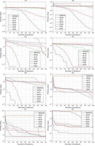
From Figure 1, the IMWOA model is confirmed to reach the fastest convergence speed in $F_1$, $F_2$, $F_3$, $F_4$ and $F_5$ tests, and its convergence value is the smallest, which is closer to 0. However, in $F_6$, the convergence value from IMWOA is slightly higher than that of MVO, but its convergence speed is still the fastest. In $F_7$ and $F_8$, IWOA has the fastest convergence speed and the smallest convergence value.

Principle of SVM Model

SVM is superior in structural risk minimization (SRM) and operation speed (Li et al. 2020). The problems caused by small samples, nonlinear and high dimensions may be avoided using SVM. It plays a key role when performing pattern recognition, classification and regression forecast (Preda et al. 2018). For prediction and classification problems, SVM can be classified as support vector classification (SVC) and support vector regression (SVR). To forecast the PV output power, SVR was used in this study, and the theory is shown below.

$\left\{(x_i,y_i)|i=1,2\cdots ,n,x_i\in R^n,y_i\in R\right\}$ is a given dataset, where $X_i$ is the input training sample, and $Y_i$ is the output training sample. The general linear regression equation of SVR is constructed as follows.

(13) $f(x)=w^T\cdot x+b$(13)

where $w$ represents the weight vector, which is the coefficient of $x$. $b$ represents a constant. x_i can be substituted into x in Equation (13)(13) $f(x)=w^T\cdot x+b$(13) for calculation, and $f(x)$ refers to the output sample value, which may produce an error compared with y_i. Both w and b are selected by the SRM principle.

To enhance the generalization ability, the promotion process is as shown below:

(14) $min\frac{1}{2}{∥w∥}^2+C{\sum }_{i=1}^m({\xi }_i+{\xi }_i^{\ast })$(14)

$s.t.\left\{\begin{array}{c}{y}_i-f(x_i)\le \epsilon +{\xi }_i\\ f(x_i)-y_i\le \epsilon +{\xi }_{{ }_i}^{\ast }\\ {\xi }_i\ge 0,{\xi }_{{ }_i}^{\ast }\ge 0\end{array}\right.$

where $\epsilon$ represents the loss function; ${\xi }_i$ and ${\xi }_i^{\ast }$ represent relaxation variables with different values; C represents the penalty coefficient; m is the number of training samples.

A Lagrangian function is established as follows:

(15) $L\left(w,b,\alpha ,{\alpha }^{\ast },\xi ,{\xi }^{\ast },\mu ,{\mu }^{\ast }\right)=\frac{1}{2}∥w∥+C\sum _{i=1}^m\left({\xi }_i+{\xi }_i^{\ast }\right)+\sum _{i=1}^m{\alpha }_i\left(f\left(x_i\right)-y_i-\epsilon -\xi \right)-\sum _{i=1}^m{\mu }_i{\xi }_i-\sum _{i=1}^m{\mu }_i^{\ast }{\xi }_i^{\ast }+\sum _{i=1}^m{\alpha }_i^{\ast }\left(y_i-f\left(x_i\right)-\epsilon -{\xi }_i^{\ast }\right)$(15)

where $\alpha$, ${\alpha }^{\ast }$, $\mu$ and ${\mu }^{\ast }$ are Lagrangian multipliers, which are greater than zero with different values (Liu et al. 2021a).

The partial derivatives of w, b, ${\xi }_i$ and ${\xi }_i^{\ast }$ are zero, which can be obtained as follows.

(16) $w={\sum }_{i=1}^m({\alpha }_i^{\ast }-{\alpha }_i)x_i$(16)

Equation (16)(16) $w={\sum }_{i=1}^m({\alpha }_i^{\ast }-{\alpha }_i)x_i$(16) is brought into Equation (13)(13) $f(x)=w^T\cdot x+b$(13) .

(17) $f(x)={\sum }_{i=1}^m({\alpha }_i^{\ast }-{\alpha }_i)x_i^{T}x+b$(17)

The PV output power is subject to many elements with multi-dimensional characteristics. To avoid this situation, a kernel function is introduced, which can display the mapped data in a high-dimensional space on the basis of the existing model.

(18) $\begin{array}{c}w({\alpha }_i,{\alpha }_i^{\ast })={\sum }_{i=1}^m({\alpha }_i-{\alpha }_i^{\ast })y_i-\epsilon {\sum }_{i=1}^m({\alpha }_i-{\alpha }_i^{\ast })\\ -\frac{1}{2}{\sum }_{i=1}^m{\sum }_{j=1}^m({\alpha }_i-{\alpha }_i^{\ast })({\alpha }_j-{\alpha }_j^{\ast })K(x_i,x_j)\end{array}$(18)

(19) $s.t.{\sum }_{i=1}^m({\alpha }_i-{\alpha }_i^{\ast })=0$(19)

where ${\alpha }_i\ge 0$, ${\alpha }_i^{\ast }\le C$.

Equation (20)(20) $w={\sum }_{i=1}^m({\alpha }_i^{\ast }-{\alpha }_i)\phi (x_i)$(20) can be obtained.

(20) $w={\sum }_{i=1}^m({\alpha }_i^{\ast }-{\alpha }_i)\phi (x_i)$(20)

The equation of the nonlinear regression model is:

(21) $f(x)={\sum }_{i=1}^m({\alpha }_i^{\ast }-{\alpha }_i)(\phi (x_i)\phi (x))+b$(21)

It can also be expressed as:

(22) $f(x)={\sum }_{i=1}^m({\alpha }_i^{\ast }-{\alpha }_i)k(x_i,x)+b$(22)

where $k(x_i,x)$ represents the kernel function.

The Gaussian kernel function is used as the kernel function in this study, shown as follows.

(23) $k(x_i,x)=exp(-\frac{{∥x_i-x∥}^2}{2{\sigma }^2})$(23)

where $\sigma$ is the bandwidth of the Gaussian kernel and is the key parameter in the kernel function.

The values of penalty coefficient (C) and key parameters of kernel function ($\sigma$) can be used to determine the regression performance of SVM. Choosing appropriate parameters can enhance the forecast performance of SVM. Therefore, this study chooses the hybrid improved whale optimization algorithm to realize the selection of SVM parameters.

Prediction of Photovoltaic Output Power by Optimizing Support Vector Machine Model with Improved Whale Algorithm

The kernel function parameter $\sigma$ and penalty coefficient $C$ in SVM can be optimized by IMWOA. The mean square error (MSE) defined in Equation (24)(24) $MSE=1\mathrm{\setminus }\mathrm{o}\mathrm{v}\mathrm{e}\mathrm{r}\mathrm{m}\sum _{i=1}^m{(s{{ }_i^{\hspace{0.17em}}}^{-}{s}_i)}^2\times 100\mathrm{\%}$(24) is used as the fitness function.

(24) $MSE=1\mathrm{\setminus }\mathrm{o}\mathrm{v}\mathrm{e}\mathrm{r}\mathrm{m}\sum _{i=1}^m{(s{{ }_i^{\hspace{0.17em}}}^{-}{s}_i)}^2\times 100\mathrm{\%}$(24)

where m is the total of test samples number, $s_i$ is the true value, and $s_i^{\hspace{0.17em}}$ is the forecast value.

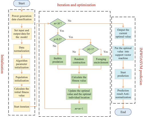
The flowchart of the prediction process is shown in Figure 2. The main process is shown as below:

1. PV power generation data is classified as test and training data sets.

2. Determine the model input and output.

3. Normalize test and training data.

4. Initialize the IMWOA model, set the number of search agents, the iteration number $M$, dimension, the search range of $C$ and $\sigma$, etc.

5. Initialize the search agent position.

6. Start iterative optimization as $M=100$.

7. Update the population position using IMWOA algorithm, calculate the fitness value of individual in each generation, and select the optimal value as the best individual of each generation.

8. The global optimal individual is selected from the best individuals in each generation since the iteration is over.

9. Input the global optimal individual into the SVM model.

10. The PV output power prediction using an optimized SVM model is implemented.

11. Anti-normalize the predicted data.

Figure 2. Flow chart of photovoltaic power output predicted by IMWOASVM model.

Prediction Results and Analysis in PV Power Generation

The data used in this study came from Desert Knowledge Australia Solar Center. The sunny data from August 8 to August 12, 2017, and the cloudy sample data from October 6 to October 10, 2017, were selected. The sample data for the first 4 days was used for training, and the sample data on the last day was used for test in both sunny and cloudy weathers. Note that the output power, weather temperature, relative humidity and light intensity between 9:00am-4:00pm were recorded every 5 minutes.

Correlation between Meteorological Elements and Output Power of PV Power Generation

To explore the influence of meteorological elements on photovoltaic power generation, sunny weather and cloudy weather are selected for investigation in this study (Liu et al. 2020). In sunny weather, the relationship between light intensity and output power, relative humidity and output power, and temperature and output power are shown in Figure 3a–c, respectively. In cloudy weather, the relationship between light intensity and output power, relative humidity and output power, and temperature and output power are shown in Figure 4a–c, respectively.

Figure 3. The relationship between meteorological elements and PV output power in sunny weather.

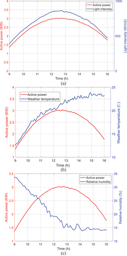
Figure 4. The relationship between meteorological elements and PV output power in cloudy weather.

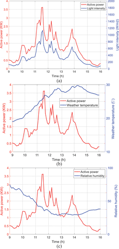
The curves from Figures 3 and 4 reveal that only light intensity has a positive correlation with the PV output power no matter on sunny or cloudy days. In order to further explore the correlation between light intensity, relative humidity, temperature and photovoltaic output power, Pearson correlation coefficient method is used to calculate the correlation between light intensity and output power, relative humidity and output power, temperature and output power (Biswas and Samanta 2021). Pearson correlation coefficient is expressed by $\rho$, and the calculation equation is shown in Equation (25)(25) $\rho =\frac{N\sum XY-\sum X\sum Y}{\sqrt{N\sum X^2-{(\sum X)}^2}\sqrt{N\sum Y^2-{(\sum Y)}^2}}$(25) ..

(25) $\rho =\frac{N\sum XY-\sum X\sum Y}{\sqrt{N\sum X^2-{(\sum X)}^2}\sqrt{N\sum Y^2-{(\sum Y)}^2}}$(25)

where $N$ represents the number of calculated samples. $X$ and $Y$ represent two variables that are used to verify the correlation strength between light intensity and output power, relative humidity and output power, weather temperature and output power. The value of $\rho$ is between [−1, 1]. The larger the absolute value of $\rho$ is, the closer it is to 1, which means that the correlation between the two variables is stronger. The correlation degree corresponding to $\rho$ is defined in Table 3 (Liu et al. 2020).

Table 3. Definition of correlation degree

$\left|\rho \right|$	correlation degree
>0.9	Almost Perfect Correlation
0.70–0.89	Very Strong Correlation
0.5–0.69	Strong Correlation
0.3–0.49	Moderate Correlation
0.10–0.29	Weak Correlation
0.01–0.09	Non-significant Correlation
0	No Correlation

The correlation values between light intensity and output power, relative humidity and output power, temperature and output power are calculated by Equation (25)(25) $\rho =\frac{N\sum XY-\sum X\sum Y}{\sqrt{N\sum X^2-{(\sum X)}^2}\sqrt{N\sum Y^2-{(\sum Y)}^2}}$(25) , as shown in Table 4.

Table 4. The value of $\rho$ in sunny and cloudy

Meteorological elements	$\rho$ in sunny	$\rho$ in cloudy
light intensity	0.9965	0.9963
relative humidity	−0.5490	−0.2219
weather temperature	0.5485	0.2759

In Table 4, the correlation between light intensity and output power is close to 1, which is almost 100% correlation in both sunny and cloudy days. When it is sunny, the correlation coefficient $\rho$ between relative humidity and output power is −0.5490, and the $\rho$ between weather temperature and output power is 0.5485. The results show a strong correlation between relative factors. If it is cloudy, the $\rho$ between relative humidity and output power is −0.2219, and the $\rho$ between weather temperature and output power is 0.2759. The results indicate a weak correlation between relative factors.

Prediction of PV Output Power

To verify the prediction effect, this study compared the proposed IMWOASVM model with other methods such as the traditional back propagation neural network model (BP), extreme learning machine model (ELM), support vector machine model (SVM), particle swarm optimization algorithm with support vector machine model (PSOSVM), genetic optimization algorithm with support vector machine model (GASVM) and whale optimization algorithm with support vector machine model (WOASVM). The light intensity, weather temperature and relative humidity which are taken as the input of the above prediction models, and the output power is taken as the output of the prediction models.

Prediction Results in Sunny Weather

In sunny weather, the results from the predicted PV output power using seven models are shown in Figure 5, and the detailed data is listed in Appendix Table A1.

Figure 5. PV output power forecast in sunny weather.

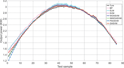
Generally, all models are confirmed to mostly fit the true value. However, in the range of samples labeled as 0–15, the results of ELM and BP models are slightly higher than the true one, and the result of PSOSVM model is lower than the true one. In the range of the 26–60th sample numbers, the prediction error of BP is significantly higher than others. As above, it can be concluded that the PSOSVM, GASVM, SVM, WOASVM and IMWOASVM models are superior to the BP and ELM models in general. The parameters of the SVM model optimized by IWOA are $C$=547.7225 and $\sigma$=0.03.

To better present the forecast results, the relative error ($\delta$) is defined as follows.

(26) $\delta =\frac{\mathrm{\Delta }s}{s}\times 100\mathrm{\%}$(26)

where $\mathrm{\Delta }s$ represents the absolute error ($\mathrm{\Delta }s=\stackrel{\wedge }{s}-s$). $\stackrel{\wedge }{s}$ denotes the predicted output power, and $s$ is the true value.

The relative error ($\delta$) curves using BP, ELM, SVM, PSOSVM, GASVM, WOASVM and IMWOASVM models in sunny weather are shown in Figure 6, and the detailed data is listed in Appendix Table A2.

Figure 6. Prediction relative error in sunny weather.

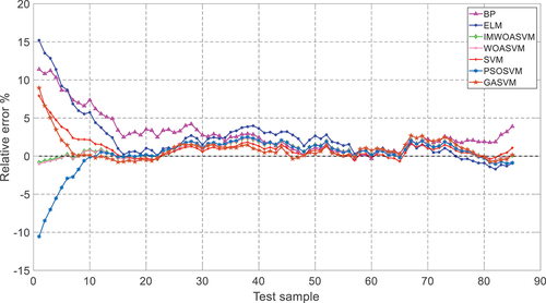
As can be seen in the range of 0–20th sample numbers, the relative errors of WOASVM and IMWOASVM are confined small between [−5%, 5%], while the errors of BP, SVM, PSOSVM, GASVM and ELM are larger, especially at the initial prediction stage. The maximum error in ELM exceeds 15%, BP exceeds 10%, and GASVM and SVM exceed 5%. In the range of 20–30th sample label, the prediction error of BP is higher than other models. In the remaining range, the errors of ELM, SVM, WOASVM and IMWOASVM models are all located between [−5%, 5%]. In conclusion as above, both WOASVM and IMWOASVM models present better prediction performance than others in sunny weather.

Prediction Results in Cloudy Weather

In cloudy weather, the PV output power forecast curves using BP, ELM, SVM, PSOSVM, GASVM, WOASVM and IMWOASVM models are shown in Figure 7, and the detailed data is listed in Appendix Table A3.

Figure 7. Output power forecast in cloudy weather.

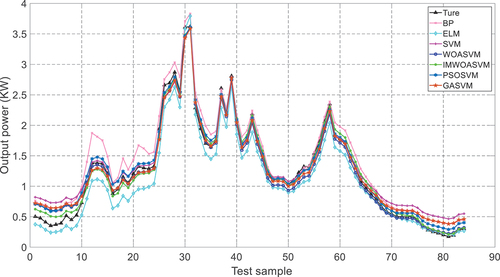
As shown in Figure 7, in the 0–10th samples, the forecast output power is not consistent with the true one, while the predicted values of ELM and IMWOASVM are closer to the true value. In the range of sample numbers between 10–40th samples, the GASVM, WOASVM and IMWOASVM models gradually fit the true output power curve. However, the prediction curves of BP and ELM models deviate far from the true one. In the samples ranged 40–70, the forecast values show a good prediction performance. In the remaining range, ELM, WOA and IMWOASVM models are closer to the true value than BP, SVM, PSOSVM, and GASVM models. As above, it is concluded that the prediction of IMWOASVM is more consistent with the true curve, indicating a better prediction effect. The parameters of the SVM model optimized by IWOA are $C$=214.7622 and $\sigma$=0.0612.

The relative errors ($\delta$) of the prediction results are shown in Figure 8, and the detailed data is listed in Appendix Table A4.

Figure 8. Prediction relative error of output power in cloudy weather.

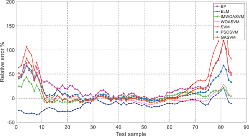
From Figure 8, it is found that all models have a significant relative error in the early and later stages during the prediction. However, the errors of ELM and IMWOASVM models are smaller than those of other models. In the range of samples between 30–60th samples, the error curves of all models begin to approach 0% gradually. During this period, the relative errors of BP, PSOSVM, GASVM, WOASVM, SVM and IMWOASVM models are small, while that of ELM model is slightly larger. In the range of samples between 60–85th samples, the errors of SVM, GASVM, PSOSVM and BP increase from the 0% baseline gradually, while the prediction error curves of ELM, WOASVM and IMWOASVM remain near 0% baseline, only slightly increasing at the end. As above, it can be concluded that the maximum errors of WOASVM and IMWOASVM appear in the starting prediction, but they are smaller than those of the other five models in the whole prediction period. Overall, the prediction error of IMWOASVM achieves the lowest value among all models.

Prediction Evaluation

To further evaluate the forecast results, the mean absolute error ($MAE$), root-mean-square error ($RMSE$) and coefficient of determination (R²) are used in this study. MAE is a measure of errors between the true value and forecasted one. RMSE is the square root of the mean of the square of all of the error. The determination coefficient R² is the proportion of the variance in the dependent variable that is predictable from the independent variable(s), and its value is confined between 0 and 1. When it is closer to 1, higher fitting degree is reached. On the contrary, the prediction has higher errors when it is closer to 0.

(27) $MAE=\frac{1}{m}\sum _i^m\left|s{{ }_i^{\hspace{0.17em}}}^{-}{s}_i\right|$(27)

(28) $RMSE=\sqrt{\frac{1}{m}\sum _{i=1}^m{(s{{ }_i^{\hspace{0.17em}}}^{-}{s}_i)}^2}\times 100\mathrm{\%}$(28)

(29) $R^2=\frac{{\left(m\sum _{i=1}^{m}ss-\sum _{i=1}^{m}s\sum _{i=1}^{m}s\right)}^2}{\left(m{\sum _{i=1}^m\left(s\right)}^2-\sum _{i=1}^m{\left(s\right)}^2\right)\left(m{\sum _{i=1}^m\left(s\right)}^2-\sum _{i=1}^m{\left(s\right)}^2\right)\times 100\mathrm{\%}}$(29)

where m is the total of test samples number, $s_i$ is the true value, and $s_i^{\hspace{0.17em}}$ is the forecast value.

The values of MAE, RMSE and R² in cloudy and sunny days are shown in Table 5, respectively.

Table 5. Evaluation of output power forecast

Weather	Model	MAE	RMSE	R^2
Sunny	BP	0.0659	7.76%	99.43%
	ELM	0.0576	5.29%	98.64%
	SVM	0.0335	2.20%	99.74%
	PSOSVM	0.0330	1.77%	99.80%
	GASVM	0.0258	2.54%	99.65%
	WOASVM	0.0253	2.19%	99.87%
	IMWOASVM	0.0251	2.17%	99.88%
Cloudy	BP	0.1731	20.01%	98.26%
	ELM	0.1708	16.37%	98.11%
	SVM	0.1298	8.50%	98.74%
	PSOSVM	0.0851	5.60%	98.95%
	GASVM	0.1002	2.38%	98.74%
	WOASVM	0.0850	2.52%	98.71%
	IMWOASVM	0.0705	1.03%	99.09%

In sunny weather, the MAE values of WOASVM and IMWOASVM models are 0.0253 and 0.0251, respectively, which are better than the other five models. From the results of RMSE, the percentages of SVM, PSOSVM, GASVM, WOASVM and IMWOASVM models are relatively small, which are 2.20%, 1.77%, 2.54%, 2.19% and 2.17%, respectively, showing better prediction accuracy. In R², all models except ELM remain above 99%.

In cloudy weather, the MAE value of IMWOASVM model achieves the smallest, i.e. 0.0705, which is the best outcome among all models. The RMSE value of IMWOASVM model is 1.03%, which is 18.98%, 15.34%, 7.47%, 4.57%, 1.35% and 1.49% lower than that of BP, ELM, SVM, PSOSVM, GASVM and WOASVM. In R², only IMWOASVM model reaches 99%.

Discussion

The PV output power is greatly affected by meteorological conditions, which may threaten the safety and stability of power system when PV generation system is connected to grid. This study aims to accurately predict PV output power and avoid the impact of PV power fluctuation to the power system.

In this work, IWOA was used to optimize the SVM model for accurately predicting the PV output power. The IWOA and six other intelligent algorithms were tested using eight test functions under the same conditions, e.g. equal population size, dimensionality, and number of iterations. Through the analysis of the test results, the IWOA was verified with faster convergence than the other tested algorithms. In addition, the convergence accuracy of IWOA was better than all other tested optimization algorithms except F6. Generally, it can be concluded that the IWOA presents the most comprehensive performance and the best search capability.

IWOASVM prediction model was developed based on the combination of IWOA with SVM. It and six other models were used to predict PV power output forecasts under sunny and cloudy weather conditions. The prediction results were evaluated using MAE, RMSE and R². During sunny weather, MAE, RMSE and R² using IWOASVM are obtained as 0.0251, 2.17% and 99.88% respectively, achieving the smallest prediction error and the best prediction result among all models. In cloudy weather, the MAE, RMSE and R² of IWOASVM are 0.0705, 1.03% and 99.09% respectively, which are better than other models.

Clearly, the IWOASVM prediction model is confirmed to be more suitable for predicting the PV output power no matter what weather conditions. Consequently, it can provide data support to reasonably arrange the power generation tasks. It is also conducive to the PV power generation efficiency, maintaining the balance between clean energy production and demand.

Conclusions

In this study, a forecast model based on IMWOA combined with SVM in short-term PV power prediction has been developed successfully. The results reveal that the proposed IMWOASVM model has a better performance than other models in PV power prediction under both sunny and cloudy days. The main contributions are concluded as follows:

1. Based on the optimization of the mutation and adaptive factors in the WOA, the proposed IMWOA has been successfully developed to upgrade the capability efficiently.

2. The test function tests verify that the IMWOA model achieves the fastest convergence speed and lowest prediction error among existing algorithms such as IMWOA, MVO, ALO, WOA, GOA, SOA and POS.

3. The IMWOA can effectively find the optimal combination of C and $\sigma$ in SVM so that the forecast ability in PV output power can be further enhanced.

4. Compared with WOASVM, ELM, SVM, GASVM, PSOSVM and BP prediction models, the IMOASVM model can reach the smallest MAE and RMSE values, and only its R² is beyond 99% under two different weather conditions.

Future research is suggested to consider more various weather conditions in a real environment. The long-term PV forecast may be advanced to further maintain the operation safety and stability in the power grid network.

Disclosure statement

No potential conflict of interest was reported by the author(s).

Correction Statement

This article has been republished with minor changes. These changes do not impact the academic content of the article.

Additional information

Funding

This study is supported by the key project of the Tianjin Natural Science Foundation [Project No. 19JCZDJC32100].

Appendix

Table A1. PV output power forecast data in sunny weather

	Ture	BP	ELM	SVM	WOASVM	IMWOASVM	PSOSVM	GASVM
1	1.3608	1.5158	1.5678	1.4686	1.3467	1.3497	1.2172	1.4827
2	1.4334	1.5884	1.6272	1.5284	1.4221	1.4248	1.3120	1.5282
3	1.5046	1.6735	1.6979	1.5906	1.4949	1.4974	1.3991	1.5806
4	1.5722	1.7343	1.7512	1.6469	1.5654	1.5676	1.4852	1.6270
5	1.6391	1.7808	1.7901	1.7021	1.6352	1.6371	1.5715	1.6734
6	1.7058	1.8523	1.8538	1.7643	1.7080	1.7097	1.6560	1.7304
7	1.7735	1.9038	1.8951	1.8157	1.7671	1.7687	1.7251	1.7787
8	1.8371	1.9656	1.9466	1.8773	1.8369	1.8383	1.8052	1.8385
9	1.8980	2.0232	2.0032	1.9397	1.9094	1.9106	1.8867	1.9007
10	1.9588	2.1028	2.0712	2.0006	1.9737	1.9748	1.9565	1.9616
11	2.0164	2.1416	2.1051	2.0485	2.0267	2.0276	2.0155	2.0120
12	2.0753	2.1905	2.1532	2.1071	2.0921	2.0929	2.0865	2.0745
13	2.1311	2.2405	2.1942	2.1551	2.1414	2.1422	2.1396	2.1256
14	2.1907	2.2984	2.2442	2.2077	2.1953	2.1960	2.1970	2.1811
15	2.2434	2.3197	2.2659	2.2463	2.2373	2.2379	2.2415	2.2260
16	2.2935	2.3506	2.2985	2.2907	2.2854	2.2860	2.2916	2.2771
17	2.3535	2.4223	2.3662	2.3508	2.3474	2.3479	2.3556	2.3400
18	2.4029	2.4788	2.4180	2.3954	2.3922	2.3926	2.4019	2.3853
19	2.4481	2.5158	2.4556	2.4411	2.4399	2.4403	2.4504	2.4373
20	2.4964	2.5843	2.5225	2.4896	2.4894	2.4896	2.5012	2.4833
21	2.5350	2.6204	2.5543	2.5243	2.5227	2.5229	2.5358	2.5197
22	2.5679	2.6318	2.5694	2.5576	2.5578	2.5580	2.5700	2.5625
23	2.6006	2.6884	2.6262	2.6048	2.6055	2.6057	2.6186	2.6090
24	2.6365	2.7284	2.6652	2.6453	2.6451	2.6453	2.6589	2.6513
25	2.6626	2.7448	2.6866	2.6801	2.6812	2.6814	2.6933	2.6943
26	2.7038	2.7928	2.7444	2.7296	2.7344	2.7344	2.7449	2.7451
27	2.7346	2.8439	2.7990	2.7663	2.7721	2.7721	2.7837	2.7755
28	2.7623	2.8788	2.8370	2.7973	2.8032	2.8031	2.8153	2.8038
29	2.7954	2.8921	2.8608	2.8244	2.8334	2.8333	2.8428	2.8347
30	2.8231	2.9009	2.8650	2.8393	2.8445	2.8445	2.8546	2.8521
31	2.8435	2.9169	2.9083	2.8713	2.8857	2.8855	2.8906	2.8834
32	2.8695	2.9525	2.9402	2.9029	2.9137	2.9136	2.9204	2.9123
33	2.9001	2.9770	2.9672	2.9266	2.9367	2.9366	2.9439	2.9331
34	2.9163	2.9735	2.9872	2.9443	2.9604	2.9602	2.9631	2.9498
35	2.9414	3.0153	3.0339	2.9774	2.9945	2.9943	2.9984	2.9744
36	2.9554	3.0307	3.0538	2.9941	3.0115	3.0113	3.0153	2.9879
37	2.9653	3.0499	3.0763	3.0161	3.0323	3.0321	3.0366	3.0068
38	2.9717	3.0587	3.0867	3.0261	3.0419	3.0417	3.0463	3.0153
39	2.9946	3.0798	3.1137	3.0423	3.0599	3.0597	3.0649	3.0248
40	3.0009	3.0743	3.1098	3.0406	3.0586	3.0584	3.0629	3.0241
41	3.0081	3.0620	3.0996	3.0362	3.0543	3.0541	3.0573	3.0221
42	3.0127	3.0671	3.1074	3.0474	3.0643	3.0642	3.0672	3.0326
43	3.0139	3.0540	3.0982	3.0412	3.0591	3.0589	3.0606	3.0274
44	2.9963	3.0541	3.0919	3.0417	3.0563	3.0562	3.0588	3.0313
45	3.0138	3.0559	3.1107	3.0465	3.0685	3.0683	3.0681	3.0258
46	3.0252	3.0532	3.1094	3.0400	3.0653	3.0651	3.0632	3.0146
47	3.0107	3.0302	3.0798	3.0212	3.0432	3.0430	3.0413	3.0050
48	2.9889	2.9928	3.0288	2.9924	3.0068	3.0067	3.0064	2.9917
49	2.9899	3.0136	3.0535	3.0092	3.0256	3.0255	3.0256	3.0039
50	2.9809	3.0137	3.0603	3.0035	3.0261	3.0259	3.0237	2.9910
51	2.9561	2.9856	3.0239	2.9790	2.9978	2.9977	2.9955	2.9749
52	2.9407	2.9850	3.0232	2.9809	2.9988	2.9987	2.9973	2.9790
53	2.9635	2.9826	3.0193	2.9777	2.9950	2.9949	2.9930	2.9751
54	2.9401	2.9594	2.9907	2.9472	2.9669	2.9667	2.9635	2.9466
55	2.9254	2.9412	2.9661	2.9248	2.9437	2.9435	2.9399	2.9269
56	2.9142	2.9342	2.9594	2.9170	2.9375	2.9373	2.9333	2.9201
57	2.9142	2.9031	2.9225	2.8980	2.9119	2.9118	2.9093	2.9102
58	2.8811	2.8851	2.9030	2.8893	2.9014	2.9014	2.9004	2.9082
59	2.8640	2.8685	2.8842	2.8733	2.8853	2.8853	2.8842	2.8943
60	2.8337	2.8241	2.8330	2.8301	2.8400	2.8400	2.8386	2.8553
61	2.8038	2.8189	2.8245	2.8099	2.8237	2.8236	2.8205	2.8320
62	2.7794	2.8061	2.8083	2.7841	2.8020	2.8018	2.7974	2.8043
63	2.7457	2.7622	2.7566	2.7390	2.7535	2.7533	2.7493	2.7624
64	2.7331	2.7523	2.7466	2.7257	2.7438	2.7435	2.7389	2.7491
65	2.7004	2.7089	2.6978	2.6818	2.6994	2.6992	2.6949	2.7074
66	2.6587	2.6941	2.6807	2.6708	2.6859	2.6857	2.6820	2.6980
67	2.6413	2.6986	2.6884	2.6839	2.6989	2.6987	2.6956	2.7128
68	2.6133	2.6556	2.6405	2.6447	2.6575	2.6573	2.6550	2.6754
69	2.5871	2.6428	2.6259	2.6262	2.6411	2.6409	2.6381	2.6559
70	2.5403	2.5975	2.5737	2.5654	2.5821	2.5818	2.5781	2.5918
71	2.4822	2.5262	2.4940	2.5045	2.5139	2.5137	2.5118	2.5314
72	2.4477	2.4956	2.4606	2.4743	2.4815	2.4814	2.4797	2.4998
73	2.4133	2.4756	2.4386	2.4493	2.4603	2.4601	2.4581	2.4735
74	2.3730	2.4291	2.3875	2.4017	2.4119	2.4116	2.4098	2.4234
75	2.3359	2.3808	2.3356	2.3531	2.3607	2.3604	2.3587	2.3715
76	2.2897	2.3300	2.2803	2.2998	2.3069	2.3065	2.3048	2.3144
77	2.2288	2.2750	2.2210	2.2389	2.2465	2.2461	2.2437	2.2486
78	2.1701	2.2152	2.1562	2.1759	2.1823	2.1818	2.1788	2.1806
79	2.1206	2.1604	2.1015	2.1204	2.1234	2.1230	2.1188	2.1209
80	2.0749	2.1143	2.0561	2.0748	2.0748	2.0743	2.0689	2.0720
81	2.0146	2.0507	1.9863	2.0073	2.0053	2.0047	1.9976	1.9998
82	1.9579	1.9945	1.9246	1.9546	1.9470	1.9465	1.9379	1.9441
83	1.8963	1.9500	1.8748	1.9008	1.8940	1.8934	1.8824	1.8874
84	1.8327	1.8913	1.8089	1.8411	1.8297	1.8290	1.8153	1.8252
85	1.7689	1.8378	1.7525	1.7882	1.7712	1.7705	1.7535	1.7717

Table A2. PV output power forecast error data in sunny weather

	BP	ELM	IMWOASVM	WOASVM	SVM	POSSVM	GASVM
1	11.3883	15.2094	−0.8181	−1.0338	7.9223	−10.5511	8.9611
2	10.8112	13.5205	−0.6013	−0.7872	6.6294	−8.4701	6.6144
3	11.2253	12.8454	−0.4760	−0.6422	5.7176	−7.0128	5.0514
4	10.3126	11.3848	−0.2928	−0.4346	4.7540	−5.5326	3.4883
5	8.6456	9.2098	−0.1214	−0.2390	3.8403	−4.1265	2.0903
6	8.5869	8.6771	0.2315	0.1304	3.4303	−2.9209	1.4450
7	7.3485	6.8606	−0.2710	−0.3593	2.3808	−2.7279	0.2947
8	6.9948	5.9646	0.0666	−0.0093	2.1926	−1.7347	0.0792
9	6.5941	5.5405	0.6632	0.6012	2.1945	−0.5955	0.1399
10	7.3536	5.7378	0.8144	0.7585	2.1352	−0.1162	0.1444
11	6.2089	4.3973	0.5571	0.5088	1.5938	−0.0469	−0.2180
12	5.5525	3.7544	0.8500	0.8107	1.5329	0.5434	−0.0349
13	5.1331	2.9632	0.5214	0.4854	1.1298	0.4025	−0.2555
14	4.9188	2.4416	0.2435	0.2112	0.7772	0.2871	−0.4372
15	3.4018	1.0028	−0.2459	−0.2739	0.1311	−0.0845	−0.7748
16	2.4892	0.2144	−0.3305	−0.3541	−0.1217	−0.0830	−0.7143
17	2.9220	0.5394	−0.2403	−0.2598	−0.1173	0.0859	−0.5767
18	3.1574	0.6283	−0.4301	−0.4475	−0.3139	−0.0444	−0.7329
19	2.7666	0.3078	−0.3175	−0.3321	−0.2826	0.0970	−0.4378
20	3.5194	1.0437	−0.2704	−0.2817	−0.2739	0.1933	−0.5253
21	3.3684	0.7608	−0.4762	−0.4868	−0.4217	0.0302	−0.6031
22	2.4912	0.0607	−0.3828	−0.3924	−0.4015	0.0845	−0.2088
23	3.3762	0.9853	0.1953	0.1881	0.1605	0.6924	0.3220
24	3.4878	1.0917	0.3343	0.3280	0.3367	0.8505	0.5609
25	3.0880	0.9003	0.7064	0.7004	0.6582	1.1540	1.1915
26	3.2929	1.5014	1.1333	1.1304	0.9542	1.5216	1.5291
27	3.9969	2.3567	1.3708	1.3707	1.1602	1.7968	1.4974
28	4.2152	2.7047	1.4768	1.4783	1.2672	1.9183	1.5023
29	3.4583	2.3392	1.3565	1.3586	1.0357	1.6950	1.4067
30	2.7544	1.4826	0.7564	0.7567	0.5715	1.1158	1.0249
31	2.5805	2.2791	1.4774	1.4812	0.9768	1.6544	1.4020
32	2.8931	2.4641	1.5381	1.5414	1.1653	1.7767	1.4934
33	2.6531	2.3147	1.2592	1.2628	0.9140	1.5128	1.1376
34	1.9609	2.4308	1.5051	1.5099	0.9587	1.6027	1.1487
35	2.5140	3.1451	1.7971	1.8038	1.2253	1.9363	1.1217
36	2.5467	3.3287	1.8900	1.8970	1.3101	2.0283	1.0984
37	2.8532	3.7439	2.2554	2.2622	1.7127	2.4049	1.4019
38	2.9271	3.8689	2.3539	2.3606	1.8282	2.5093	1.4668
39	2.8442	3.9786	2.1737	2.1822	1.5916	2.3471	1.0071
40	2.4484	3.6294	1.9164	1.9245	1.3253	2.0671	0.7745
41	1.7931	3.0438	1.5297	1.5367	0.9350	1.6384	0.4675
42	1.8082	3.1439	1.7094	1.7155	1.1531	1.8099	0.6628
43	1.3310	2.7983	1.4950	1.5006	0.9072	1.5490	0.4492
44	1.9278	3.1900	1.9975	2.0016	1.5152	2.0836	1.1655
45	1.3972	3.2150	1.8087	1.8156	1.0856	1.8005	0.3968
46	0.9271	2.7841	1.3182	1.3263	0.4892	1.2568	−0.3518
47	0.6504	2.2954	1.0727	1.0790	0.3513	1.0171	−0.1872
48	0.1281	1.3330	0.5944	0.5966	0.1159	0.5850	0.0932
49	0.7902	2.1269	1.1897	1.1933	0.6451	1.1922	0.4687
50	1.0983	2.6624	1.5071	1.5138	0.7575	1.4335	0.3365
51	1.0003	2.2934	1.4077	1.4123	0.7771	1.3350	0.6384
52	1.5071	2.8067	1.9738	1.9779	1.3692	1.9245	1.3049
53	0.6449	1.8838	1.0609	1.0646	0.4804	0.9975	0.3914
54	0.6568	1.7234	0.9061	0.9115	0.2418	0.7957	0.2238
55	0.5386	1.3913	0.6202	0.6256	−0.0220	0.4947	0.0504
56	0.6847	1.5521	0.7943	0.8005	0.0970	0.6565	0.2009
57	−0.3806	0.2848	−0.0827	−0.0804	−0.5560	−0.1689	−0.1362
58	0.1397	0.7600	0.7061	0.7067	0.2845	0.6712	0.9419
59	0.1561	0.7045	0.7423	0.7427	0.3248	0.7042	1.0594
60	−0.3393	−0.0270	0.2200	0.2196	−0.1267	0.1704	0.7624
61	0.5402	0.7387	0.7072	0.7104	0.2161	0.5958	1.0053
62	0.9600	1.0389	0.8072	0.8140	0.1689	0.6471	0.8971
63	0.6004	0.3950	0.2758	0.2821	−0.2453	0.1298	0.6067
64	0.7004	0.4940	0.3803	0.3885	−0.2721	0.2128	0.5848
65	0.3153	−0.0947	−0.0454	−0.0367	−0.6904	−0.2046	0.2604
66	1.3301	0.8269	1.0160	1.0233	0.4537	0.8767	1.4758
67	2.1680	1.7814	2.1727	2.1783	1.6123	2.0543	2.7054
68	1.6189	1.0379	1.6841	1.6887	1.2017	1.5929	2.3743
69	2.1517	1.4967	2.0776	2.0841	1.5101	1.9690	2.6572
70	2.2504	1.3138	1.6338	1.6451	0.9866	1.4883	2.0257
71	1.7742	0.4746	1.2694	1.2772	0.8964	1.1918	1.9807
72	1.9545	0.5242	1.3736	1.3813	1.0839	1.3068	2.1288
73	2.5799	1.0455	1.9368	1.9471	1.4901	1.8549	2.4949
74	2.3622	0.6129	1.6267	1.6379	1.2095	1.5525	2.1222
75	1.9211	−0.0158	1.0471	1.0590	0.7339	0.9762	1.5240
76	1.7578	−0.4138	0.7342	0.7480	0.4383	0.6560	1.0767
77	2.0724	−0.3514	0.7766	0.7940	0.4524	0.6682	0.8878
78	2.0778	−0.6403	0.5386	0.5586	0.2656	0.3971	0.4815
79	1.8749	−0.9017	0.1114	0.1343	−0.0072	−0.0870	0.0127
80	1.8997	−0.9040	−0.0268	−0.0016	−0.0024	−0.2858	−0.1389
81	1.7910	−1.4027	−0.4911	−0.4625	−0.3621	−0.8444	−0.7327
82	1.8671	−1.7016	−0.5852	−0.5571	−0.1709	−1.0245	−0.7046
83	2.8281	−1.1356	−0.1573	−0.1230	0.2381	−0.7338	−0.4722
84	3.1980	−1.2992	−0.2044	−0.1681	0.4543	−0.9503	−0.4087
85	3.8948	−0.9243	0.0920	0.1309	1.0942	−0.8660	0.1576

Table A3. PV output power forecast data in cloudy weather

	Ture	BP	ELM	SVM	WOASVM	IMWOASVM	PSOSVM	GASVM
1	0.5022	0.7643	0.3748	0.8207	0.7121	0.6245	0.7058	0.7232
2	0.4760	0.6950	0.3500	0.8000	0.6862	0.5878	0.6839	0.7059
3	0.4115	0.6962	0.2858	0.7665	0.6470	0.5621	0.6347	0.6745
4	0.3526	0.6085	0.2406	0.7288	0.6025	0.5074	0.5887	0.6429
5	0.3717	0.5867	0.2509	0.7312	0.6029	0.4983	0.5976	0.6448
6	0.3938	0.6004	0.2712	0.7456	0.6175	0.5103	0.6197	0.6565
7	0.5173	0.7325	0.3516	0.8132	0.6918	0.5924	0.7103	0.7128
8	0.4497	0.7368	0.2971	0.7839	0.6588	0.5720	0.6661	0.6853
9	0.5251	0.8009	0.3533	0.8248	0.7035	0.6147	0.7231	0.7203
10	0.7292	0.9928	0.5271	0.9499	0.8406	0.7444	0.8943	0.8321
11	1.0494	1.4002	0.7965	1.1576	1.0681	0.9758	1.1625	1.0268
12	1.3811	1.8734	1.0907	1.3952	1.3278	1.2513	1.4504	1.2631
13	1.3803	1.8132	1.1134	1.4195	1.3520	1.2779	1.4781	1.2973
14	1.3748	1.7536	1.0803	1.3950	1.3237	1.2489	1.4492	1.2738
15	1.2091	1.4919	0.9362	1.2818	1.1950	1.1139	1.3159	1.1636
16	0.8790	1.0592	0.6391	1.0479	0.9266	0.8379	1.0333	0.9322
17	0.9512	1.1370	0.6842	1.0865	0.9696	0.8849	1.0804	0.9698
18	1.1532	1.4580	0.8415	1.2243	1.1223	1.0539	1.2451	1.1039
19	1.0567	1.2734	0.7600	1.1561	1.0409	0.9745	1.1638	1.0408
20	1.2052	1.4360	0.8834	1.2580	1.1535	1.0989	1.2837	1.1470
21	1.3234	1.6703	0.9517	1.3339	1.2317	1.1994	1.3685	1.2222
22	1.3005	1.6213	0.9616	1.3382	1.2342	1.2089	1.3718	1.2321
23	1.2868	1.5317	0.9885	1.3451	1.2445	1.2161	1.3802	1.2457
24	1.3298	1.5624	1.0439	1.3872	1.2912	1.2705	1.4267	1.2938
25	1.9407	2.1505	1.5486	1.8217	1.7757	1.7905	1.8983	1.7656
26	2.6612	2.7570	2.2982	2.4498	2.4599	2.4985	2.5348	2.4556
27	2.6939	2.8696	2.4225	2.5552	2.5687	2.6091	2.6364	2.5684
28	2.8714	3.0311	2.6259	2.7157	2.7384	2.7775	2.7940	2.7362
29	2.5635	2.7902	2.2985	2.4664	2.4658	2.5125	2.5417	2.4765
30	3.6095	3.7081	3.5792	3.4293	3.4570	3.4864	3.4702	3.4363
31	3.6201	3.8314	3.7925	3.5942	3.5983	3.5880	3.6116	3.5870
32	2.2853	2.5354	2.1762	2.3568	2.3483	2.4100	2.4187	2.3756
33	1.9433	2.2438	1.8023	2.0342	1.9979	2.0708	2.0936	2.0224
34	1.7021	1.9877	1.5283	1.7882	1.7276	1.7982	1.8391	1.7517
35	1.6454	1.8506	1.4473	1.7041	1.6388	1.6989	1.7526	1.6603
36	1.7600	1.9020	1.5277	1.7673	1.7096	1.7792	1.8165	1.7329
37	2.6080	2.5877	2.2869	2.4453	2.4453	2.5018	2.5055	2.4735
38	2.1829	2.2772	1.9744	2.1614	2.1428	2.2189	2.2183	2.1694
39	2.8106	2.7968	2.6368	2.7263	2.7445	2.7758	2.7762	2.7757
40	2.0797	2.1811	1.8533	2.0467	2.0112	2.1141	2.0915	2.0467
41	1.7035	1.8131	1.4680	1.6678	1.5924	1.7253	1.6876	1.6361
42	1.7417	1.9133	1.5781	1.7728	1.7099	1.8381	1.8004	1.7504
43	2.1876	2.2403	1.8845	2.0793	2.0404	2.1562	2.1187	2.0831
44	1.7657	1.9157	1.5703	1.7587	1.6923	1.8366	1.7796	1.7375
45	1.5064	1.6554	1.3445	1.5258	1.4356	1.5813	1.5291	1.4856
46	1.2004	1.3122	1.0855	1.2588	1.1365	1.2647	1.2349	1.1979
47	1.0992	1.1359	0.9820	1.1506	1.0153	1.1187	1.1165	1.0804
48	1.1233	1.1396	0.9713	1.1570	1.0216	1.1158	1.1274	1.0845
49	1.1305	1.1405	0.9585	1.1499	1.0125	1.1086	1.1188	1.0769
50	1.0366	1.0284	0.8975	1.0783	0.9322	1.0168	1.0370	1.0014
51	1.0978	1.0633	0.9206	1.1089	0.9671	1.0490	1.0743	1.0323
52	1.2250	1.1751	1.0030	1.1921	1.0620	1.1525	1.1694	1.1205
53	1.3232	1.3080	1.0725	1.2724	1.1512	1.2560	1.2586	1.2066
54	1.3255	1.3302	1.0984	1.2887	1.1703	1.2818	1.2749	1.2256
55	1.5388	1.5603	1.2661	1.4600	1.3624	1.4888	1.4633	1.4107
56	1.7294	1.7955	1.4410	1.6425	1.5633	1.7006	1.6590	1.6091
57	2.0616	2.1380	1.7577	1.9554	1.9029	2.0422	1.9848	1.9504
58	2.3492	2.3882	2.0365	2.2173	2.1817	2.3056	2.2498	2.2337
59	1.8350	2.0441	1.6403	1.8399	1.7751	1.9331	1.8595	1.8269
60	1.7772	1.9764	1.5773	1.7816	1.7125	1.8635	1.8016	1.7621
61	1.7135	1.9165	1.5151	1.7183	1.6428	1.8000	1.7329	1.6943
62	1.4860	1.7169	1.3067	1.5109	1.4119	1.5836	1.5047	1.4728
63	1.2953	1.5100	1.1548	1.3390	1.2222	1.3988	1.3109	1.2923
64	1.0743	1.2857	0.9942	1.1687	1.0315	1.1974	1.1184	1.1125
65	0.9707	1.1575	0.9042	1.0797	0.9305	1.0823	1.0183	1.0175
66	0.8702	1.0332	0.8182	0.9916	0.8304	0.9699	0.9165	0.9252
67	0.7830	0.9355	0.7447	0.9173	0.7457	0.8765	0.8288	0.8489
68	0.6631	0.8034	0.6425	0.8195	0.6332	0.7453	0.7138	0.7475
69	0.5886	0.7086	0.5721	0.7575	0.5613	0.6496	0.6434	0.6807
70	0.5440	0.6631	0.5241	0.7184	0.5157	0.5950	0.5968	0.6405
71	0.5055	0.6250	0.4804	0.6875	0.4795	0.5476	0.5612	0.6077
72	0.5001	0.6167	0.4653	0.6871	0.4783	0.5364	0.5640	0.6043
73	0.5007	0.6046	0.4418	0.6798	0.4692	0.5183	0.5577	0.5946
74	0.5027	0.6114	0.4303	0.6837	0.4730	0.5195	0.5637	0.5971
75	0.4471	0.5668	0.3925	0.6474	0.4315	0.4680	0.5197	0.5606
76	0.3334	0.4908	0.3230	0.5760	0.3496	0.3714	0.4304	0.4909
77	0.2807	0.4543	0.2889	0.5402	0.3086	0.3217	0.3854	0.4562
78	0.2513	0.4334	0.2668	0.5187	0.2838	0.2912	0.3582	0.4353
79	0.2307	0.4128	0.2545	0.5009	0.2636	0.2639	0.3361	0.4179
80	0.2020	0.3959	0.2330	0.4823	0.2423	0.2367	0.3128	0.3999
81	0.1737	0.3811	0.2111	0.4653	0.2226	0.2113	0.2914	0.3833
82	0.1946	0.3911	0.2077	0.4785	0.2377	0.2246	0.3096	0.3946
83	0.2818	0.4364	0.2593	0.5379	0.3063	0.2979	0.3877	0.4498
84	0.3031	0.4487	0.2686	0.5503	0.3204	0.3145	0.4035	0.4615

Table A4. PV output power forecast error data in cloudy weather

	BP	ELM	IMWOASVM	WOASVM	SVM	POSSVM	GASVM
1	52.1940	−25.3648	24.3436	41.7943	63.4230	40.5493	44.0015
2	46.0124	−26.4575	23.4951	44.1644	68.0823	43.6818	48.3051
3	69.1826	−30.5429	36.5866	57.2281	86.2770	54.2522	63.9156
4	72.5828	−31.7460	43.9255	70.8973	106.7176	66.9653	82.3404
5	57.8372	−32.4992	34.0723	62.1940	96.7266	60.7816	73.4695
6	52.4391	−31.1358	29.5618	56.7840	89.3153	57.3536	66.7073
7	41.5826	−32.0295	14.5087	33.7266	57.1982	37.3023	37.7795
8	63.8352	−33.9286	27.1838	46.4838	74.2965	48.1082	52.3704
9	52.5350	−32.7122	17.0786	33.9742	57.0793	37.7143	37.1807
10	36.1424	−27.7105	2.0849	15.2798	30.2610	22.6372	14.1180
11	33.4328	−24.1014	−7.0133	1.7870	10.3136	10.7766	−2.1532
12	35.6494	−21.0256	−9.3951	−3.8563	1.0198	5.0225	−8.5447
13	31.3579	−19.3364	−7.4182	−2.0525	2.8353	7.0793	−6.0154
14	27.5560	−21.4171	−9.1560	−3.7117	1.4683	5.4123	−7.3420
15	23.3956	−22.5688	−7.8729	−1.1645	6.0197	8.8349	−3.7600
16	20.5027	−27.2924	−4.6780	5.4134	19.2121	17.5544	6.0529
17	19.5381	−28.0645	−6.9644	1.9357	14.2277	13.5867	1.9538
18	26.4288	−27.0251	−8.6109	−2.6828	6.1678	7.9695	−4.2792
19	20.5066	−28.0795	−7.7859	−1.4976	9.4042	10.1284	−1.5062
20	19.1554	−26.6974	−8.8195	−4.2876	4.3862	6.5194	−4.8271
21	26.2179	−28.0813	−9.3642	−6.9297	0.7990	3.4077	−7.6468
22	24.6644	−26.0604	−7.0460	−5.0975	2.8962	5.4841	−5.2620
23	19.0295	−23.1810	−5.4907	−3.2879	4.5312	7.2615	−3.1917
24	17.4890	−21.4993	−4.4621	−2.9053	4.3131	7.2841	−2.7077
25	10.8093	−20.2071	−7.7413	−8.5014	−6.1340	−2.1856	−9.0241
26	3.6004	−13.6410	−6.1140	−7.5623	−7.9428	−4.7484	−7.7244
27	6.5206	−10.0739	−3.1505	−4.6479	−5.1487	−2.1354	−4.6607
28	5.5590	−8.5508	−3.2710	−4.6332	−5.4237	−2.6957	−4.7111
29	8.8434	−10.3357	−1.9893	−3.8094	−3.7895	−0.8512	−3.3919
30	2.7316	−0.8399	−3.4125	−4.2270	−4.9938	−3.8603	−4.7992
31	5.8345	4.7612	−0.8885	−0.6020	−0.7165	−0.2362	−0.9152
32	10.9407	−4.7754	5.4546	2.7548	3.1257	5.8343	3.9505
33	15.4630	−7.2558	6.5623	2.8091	4.6759	7.7328	4.0723
34	16.7816	−10.2104	5.6480	1.4985	5.0607	8.0538	2.9149
35	12.4668	−12.0386	3.2481	−0.4057	3.5627	6.5109	0.9065
36	8.0704	−13.2005	1.0890	−2.8610	0.4174	3.2093	−1.5420
37	−0.7754	−12.3101	−4.0718	−6.2364	−6.2361	−3.9292	−5.1545
38	4.3166	−9.5520	1.6476	−1.8377	−0.9876	1.6194	−0.6185
39	−0.4887	−6.1841	−1.2361	−2.3499	−2.9982	−1.2238	−1.2411
40	4.8735	−10.8843	1.6542	−3.2920	−1.5890	0.5698	−1.5866
41	6.4293	−13.8278	1.2760	−6.5233	−2.0992	−0.9377	−3.9598
42	9.8548	−9.3933	5.5346	−1.8242	1.7880	3.3695	0.4995
43	2.4108	−13.8555	−1.4334	−6.7289	−4.9498	−3.1479	−4.7790
44	8.4939	−11.0648	4.0146	−4.1576	−0.3975	0.7884	−1.5951
45	9.8891	−10.7442	4.9729	−4.7032	1.2885	1.5062	−1.3824
46	9.3120	−9.5734	5.3569	−5.3238	4.8625	2.8733	−0.2048
47	3.3317	−10.6694	1.7703	−7.6364	4.6728	1.5726	−1.7171
48	1.4511	−13.5312	−0.6725	−9.0559	2.9970	0.3597	−3.4609
49	0.8915	−15.2086	−1.9353	−10.4312	1.7159	−1.0343	−4.7361
50	−0.7914	−13.4213	−1.9098	−10.0748	4.0159	0.0387	−3.4025
51	−3.1470	−16.1387	−4.4465	−11.9050	1.0115	−2.1370	−5.9688
52	−4.0740	−18.1248	−5.9232	−13.3059	−2.6915	−4.5416	−8.5371
53	−1.1473	−18.9454	−5.0804	−13.0004	−3.8384	−4.8846	−8.8114
54	0.3540	−17.1328	−3.2973	−11.7093	−2.7715	−3.8151	−7.5346
55	1.3947	−17.7185	−3.2499	−11.4664	−5.1186	−4.9076	−8.3237
56	3.8197	−16.6736	−1.6632	−9.6044	−5.0244	−4.0686	−6.9563
57	3.7066	−14.7398	−0.9400	−7.6958	−5.1521	−3.7268	−5.3930
58	1.6589	−13.3113	−1.8569	−7.1317	−5.6165	−4.2310	−4.9147
59	11.3956	−10.6115	5.3456	−3.2653	0.2668	1.3325	−0.4390
60	11.2114	−11.2444	4.8607	−3.6361	0.2470	1.3728	−0.8498
61	11.8462	−11.5790	5.0493	−4.1275	0.2817	1.1294	−1.1188
62	15.5355	−12.0679	6.5636	−4.9897	1.6767	1.2593	−0.8933
63	16.5774	−10.8414	7.9957	−5.6431	3.3728	1.2078	−0.2327
64	19.6784	−7.4551	11.4550	−3.9887	8.7801	4.1002	3.5530
65	19.2519	−6.8426	11.5053	−4.1367	11.2292	4.9024	4.8214
66	18.7290	−5.9779	11.4555	−4.5732	13.9453	5.3264	6.3184
67	19.4756	−4.8896	11.9389	−4.7712	17.1503	5.8506	8.4109
68	21.1621	−3.0988	12.3993	−4.5042	23.5922	7.6482	12.7352
69	20.3963	−2.7977	10.3654	−4.6367	28.6954	9.3223	15.6529
70	21.9015	−3.6608	9.3855	−5.1932	32.0623	9.7173	17.7413
71	23.6575	−4.9587	8.3425	−5.1424	36.0212	11.0168	20.2279
72	23.3240	−6.9591	7.2705	−4.3550	37.4087	12.7935	20.8379
73	20.7536	−11.7635	3.5190	−6.2857	35.7739	11.3775	18.7568
74	21.6265	−14.3943	3.3492	−5.9081	35.9990	12.1427	18.7737
75	26.7818	−12.2042	4.6742	−3.4790	44.8184	16.2574	25.4010
76	47.2223	−3.1002	11.4061	4.8643	72.7768	29.0951	47.2454
77	61.8806	2.9304	14.6200	9.9512	92.4813	37.3119	62.5362
78	72.4879	6.1658	15.8770	12.9624	106.4248	42.5757	73.2348
79	78.9476	10.3311	14.4173	14.2905	117.1500	45.7188	81.1776
80	95.9819	15.3634	17.1690	19.9381	138.7849	54.8497	97.9676
81	119.3839	21.5089	21.6367	28.1709	167.8776	67.7422	120.6799
82	100.9561	6.7215	15.4078	22.1210	145.8266	59.0925	102.7468
83	54.8969	−7.9649	5.7319	8.6926	90.8998	37.5914	59.6231
84	48.0442	−11.3986	3.7674	5.7168	81.5509	33.1365	52.2685

References

- Al-Dahidi, S., O. Ayadi, J. Adeeb, M. Alrbai, and B. R. Qawasmeh. 2018. Extreme learning machines for solar photovoltaic power predictions. Energies 11 (10):2725. doi:10.3390/en11102725.
- Al-Dahidi, S., O. Ayadi, J. Adeeb, and M. Louzazni. 2019. Assessment of artificial neural networks learning algorithms and training datasets for solar photovoltaic power production prediction. Frontiers in Energy Research 7. doi:10.3389/fenrg.2019.00130.
- Bae, K. Y., S. J. Han, C. J. Bang, and K. S. Dan. 2019. Effect of prediction error of machine learning schemes on photovoltaic power trading based on energy storage systems. Energies 12:1249. doi:10.3390/en12071249.
- Biswas, P., and T. Samanta. 2021. A method for fault detection in wireless sensor network based on pearson’s correlation coefficient and support vector machine classification. Wireless Personal Communications. doi:10.1007/s11277-021-09257-7.
- Carvajal-Romo, G., M. Valderrama-Mendoza, D. Rodriguez-Urrego, and L. Rodriguez-Urrego. 2019. Assessment of solar and wind energy potential in La Guajira, Colombia: Current status, and future prospects. Sustainable Energy Technologies 36:100531. doi:10.1016/j.seta.2019.100531.
- Chai, M. K., F. Xia, S. T. Hao, D. G. Peng, C. G. Cui, and W. Liu. 2019. PV power prediction based on LSTM with adaptive hyperparameter adjustment. Ieee Access 7:115473–1226. doi:10.1109/ACCESS.2019.2936597.
- Cheng, Z., Q. Liu, and W. Zhang. 2019. Improved probability prediction method research for photovoltaic power output. Applied Sciences Basel 9(10):2043. doi:10.3390/app9102043.
- Dhiman, G., and V. Kumar. 2019. Seagull optimization algorithm: Theory and its applications for large-scale industrial engineering problems. Knowledge-Based Systems 165:169–96. doi:10.1016/j.knosys.2018.11.024.
- Eseye, A. T., J. H. Zhang, and D. H. Zheng. 2018. Short-term photovoltaic solar power forecasting using a hybrid wavelet-PSO-SVM model based on SCADA and meteorological information. Renewable Energy 118:357–67. doi:10.1016/j.renene.2017.11.011.
- Gandoman, F. H., F. Raeisi, and A. Ahmadi. 2016. A literature review on estimating of PV-array hourly power under cloudy weather conditions. Renewable and Sustainable Energy Reviews 63:579–92. doi:10.1016/j.rser.2016.05.027.
- Gao, M. M., J. J. Li, F. Hong, and D. T. Long. 2019. Day-ahead power forecasting in a large-scale photovoltaic plant based on weather classification using LSTM. Energy 187:115838. doi:10.1016/j.energy.2019.07.168.
- Gao, Z. K., J. Q. Yu, A. J. Zhao, Q. Hu, and S. Yang. 2022. A hybrid method of cooling load forecasting for large commercial. Energy 238:122073. doi:10.1016/j.energy.2021.122073.
- Gurung, S., S. Naetiladdanon, and A. Sangswang. 2019. Probabilistic small-signal stability analysis of power system with solar farm integration. Turkish Journal of Electrical Engineering Computer 27:1276–89. doi:10.3906/elk-1804-228.
- Han, Y. T., N. B. Wang, M. Ma, H. Zhou, S. Y. Dai, and H. L. Zhu. 2019. A PV power interval forecasting based on seasonal model and nonparametric estimation algorithm. Solar Energy 184:515–26. doi:10.1016/j.solener.2019.04.025.
- He, X. X., S. Y. Yuan, W. B. Li, H. Yang, W. Ji, Z. Q. Wang, J. Y. Hao, C. Chen, W. Q. Chen, Y. X. Gao, et al. 2019. Improvement of Asia-Pacific colorectal screening score and evaluation of its use combined with fecal immunochemical test. BMC Gastroenterology 19. doi:10.1186/s12876-019-1146-2.
- Hua, C., E. X. Zhu, L. Kuang, and D. C. Pi. 2019. Short-term power prediction of photovoltaic power station based on long short-term memory-back-propagation. International Journal of Distributed Sensor Networks 15(10):1550147719883134. doi:10.1177/1550147719883134.
- Li, J. M., J. K. Ward, J. N. Tong, L. Collins, and G. Platt. 2016. Machine learning for solar irradiance forecasting of photovoltaic system. Renewable Energy 90:542–53. doi:10.1016/j.renene.2015.12.069.
- Li, L. L., S. Y. Wen, M. L. Tseng, and C. S. Wang. 2019. Renewable energy prediction: A novel short-term prediction model of photovoltaic output power. Journal of Cleaner Production 228:359–75. doi:10.1016/j.jclepro.2019.04.331.
- Li, L. L., X. Zhao, M. L. Tseng, and R. T. Raymond. 2020. Short-term wind power forecasting based on support vector machine with improved dragonfly algorithm. Journal of Cleaner Production 242:118447. doi: 10.1016/j.jclepro.2019.118447.
- Li, L. L., Z. F. Liu, M. L. Tseng, S. J. Zheng, and M. K. Lim. 2021a. Improved tunicate swarm algorithm: Solving the dynamic economic emission dispatch problems. Applied Soft Computing 108:107504. doi:10.1016/j.asoc.2021.107504.
- Lin, P. J., Z. N. Peng, Y. F. Lai, S. Y. Cheng, Z. C. Chen, and L. J. Wu. 2018. Short-term power prediction for photovoltaic power plants using a hybrid improved Kmeans-GRA-Elman model based on multivariate meteorological factors and historical power datasets. Energy Conversion and Management 177:704–17. doi:10.1016/j.enconman.2018.10.015.
- Liu, L. P., M. M. Zhan, and Y. Bai. 2019. A recursive ensemble model for forecasting the power output of photovoltaic systems. Solar Energy 189:291–98. doi:10.1016/j.solener.2019.07.061.
- Liu, L. Y., Y. Zhao, D. L. Chang, J. Y. Xie, Z. Y. Ma, Q. Sun, H. Y. Yin, and R. Wennersten. 2018. Prediction of short-term PV power output and uncertainty analysis. Applied Energy 228:700–11. doi:10.1016/j.apenergy.2018.06.112.
- Liu, Y. W., H. Feng, H. Y. Li, and L. L. Li. 2021a. An improved whale algorithm for support vector machine prediction of photovoltaic power generation. Symmetry 13(2):212. doi:10.3390/sym13020212.
- Liu, Z. F., L. L. Li, M. L. Tseng, and M. K. Lim. 2020. Prediction short-term photovoltaic power using improved chicken swarm optimizer - Extreme learning machine model. Journal of Cleaner Production 248:119272. doi:10.1016/j.jclepro.2019.119272.
- Liu, Z. F., L. L. Li, Y. W. Liu, J. Q. Liu, H. Y. Li, and Q. Shen. 2021b. Dynamic economic emission dispatch considering renewable energy generation: A novel multi-objective optimization approach. Energy 235:121407. doi:10.1016/j.energy.2021.121407.
- Mirjalili, S., and A. Lewis. 2016a. The whale optimization algorithm. Advances in Engineering Software 95:51–67. doi:10.1016/j.advengsoft.2016.01.008.
- Mirjalili, S., S. M. Mirjalili, and A. Hatamlou. 2016b. Multi-verse optimizer: A nature-inspired algorithm for global optimization. Neural Computing & Applications 27:495–513. doi:10.1007/s00521-015-1870-7.
- Mirjalili, S. 2015. The ant lion optimizer. Advances in Engineering Software 83:80–98. doi:10.1016/j.advengsoft.2015.01.010.
- Mojumder, J. C., H. C. Ong, W. T. Chong, S. Shamshirband, and A. Al-Mamoon. 2016. Application of support vector machine for prediction of electrical and thermal performance in PV/T system. Energy and Buildings 111:267–77. doi:10.1016/j.enbuild.2015.11.043.
- Monfared, M., M. Fazeli, R. Lewis, and J. Searle. 2019. Fuzzy predictor with additive learning for very short-term PV power generation. Ieee Access 7:91183–92. doi:10.1109/ACCESS.2019.2927804.
- Ni, Q., S. X. Zhuang, H. M. Sheng, S. Wang, and J. Xiao. 2017. An optimized prediction intervals approach for short term PV power forecasting. Energies 10 (10):1669. doi:10.3390/en10101669.
- Pierro, M., M. De Felice, E. Maggioni, D. Moser, A. Perotto, F. Spade, and C. Cornaro. 2017. Data-driven upscaling methods for regional photovoltaic power estimation and forecast using satellite and numerical weather prediction data. Solar Energy 158:1026–38. doi:10.1016/j.solener.2017.09.068.
- Preda, S., S. V. Oprea, A. Bâra, and A. Belciu. 2018. PV forecasting using support vector machine learning in a big data analytics context. Symmetry 10:748. doi:10.3390/sym10120748.
- Rana, M., I. Koprinska, and V. G. Agelidis. 2016. Univariate and multivariate methods for very short-term solar photovoltaic power forecasting. Energy Conversion and Management 121:380–90. doi:10.1016/j.enconman.2016.05.025.
- Raza, M. Q., M. Nadarajah, and C. Ekanayake. 2017. Demand forecast of PV integrated bioclimatic buildings using ensemble framework. Applied Energy 208:1626–38. doi:10.1016/j.apenergy.2017.08.192.
- Semero, Y. K., D. H. Zheng, and J. H. Zhang. 2018. A PSO-ANFIS based hybrid approach for short term PV power prediction in microgrids. Electric Power Components and Systems 46:95–103. doi:10.1080/15325008.2018.1433733.
- Shahrzad, S., S. Mirjalili, and A. Lewis. 2017. Grasshopper optimisation algorithm: Theory and application. Advances in Engineering Software 105:30–47. doi:10.1016/j.advengsoft.2017.01.004.
- Simhadri, K. S., and B. Mohanty. 2019. Performance analysis of dual-mode PI controller using quasi-oppositional whale optimization algorithm for load frequency control. International Transactions on Electrical Energy 30 (1):e12159. doi:10.1002/2050-7038.12159.
- van der Meer, D. W., M. Shepero, A. Svensson, J. Widen, and J. Munkhammar. 2018. Probabilistic forecasting of electricity consumption, photovoltaic power generation and net demand of an individual building using Gaussian Processes. Applied Energy 213:195–207. doi:10.1016/j.apenergy.2017.12.104.
- VanDeventer, W., E. Jamei, G. S. Thirunavukkarasu, M. Seyedmahmoudian, T. K. Soon, B. Horan, S. Mekhilef, and A. Stojcevski. 2019. Short-term PV power forecasting using hybrid GASVM technique. Renewable Energy 140:367–79. doi:10.1016/j.renene.2019.02.087.
- Wang, F., Z. Zhen, C. Liu, Z. Q. Mi, M. Shafie-khah, and J. P. S. Catalao. 2018a. Time-section fusion pattern classification based day-ahead solar irradiance ensemble forecasting model using mutual iterative optimization. Energies 11(1):184. doi:10.3390/en11010184.
- Wang, K. J., X. X. Qi, and H. D. Liu. 2019. A comparison of day-ahead photovoltaic power forecasting models based on deep learning neural network. Applied Energy 251:113315. doi:10.1016/j.apenergy.2019.113315.
- Wang, Q., S. X. Ji, M. Q. Hu, W. Li, F. S. Liu, and L. Zhu. 2018b. Short-term photovoltaic power generation combination forecasting method based on similar day and cross entropy theory. International Journal of Photoenergy 2018:1–10. doi:10.1155/2018/6973297.
- Xie, T., G. Zhang, H. C. Liu, F. C. Liu, and P. D. Du. 2018. A hybrid forecasting method for solar output power based on variational mode decomposition, deep belief networks and auto-regressive moving average. Applied Sciences Basel 8 (10):1901. doi:10.3390/app8101901.
- Xiong, X., X. Hu, and H. Guo. 2021. A hybrid optimized grey seasonal variation index model improved by whale optimization algorithm for forecasting the residential electricity consumption. Energy 4:121127. doi:10.1016/j.energy.2021.121127.
- Yang, S. X., X. G. Zhu, and S. J. Peng. 2020. Prospect prediction of terminal clean power consumption in China via LSSVM algorithm based on improved evolutionary game theory. Energies 13 (8):2065. doi:10.3390/en13082065.
- Yu, M., F. C. Chen, S. M. Zheng, J. Z. Zhou, X. D. Zhao, Z. Y. Wang, G. Q. Li, J. Li, Y. Fan, J. Ji, et al. 2019. Experimental investigation of a novel solar micro-channel loop-heat-pipe photovoltaic/thermal (MC-LHP-PV/T) system for heat and power generation. Applied Energy 256:113929. doi:10.1016/j.apenergy.2019.113929.
- Yuan, P. L., C. J. Guo, Q. Zheng, and J. Ding. 2018. Sidelobe suppression with constraint for MIMO radar via chaotic whale optimisation. Electronics Letters 54 (5):311–13. doi:10.1049/el.2017.4286.
- Zhang, X. Z., Z. Y. Wang, and Z. Lu. 2022. Multi-objective load dispatch for microgrid with electric vehicles using modified gravitational search and particle swarm optimization algorithm. Applied Energy 306:118018. doi:10.1016/j.apenergy.2021.118018.