A Comparative Assessment of Deep Neural Network Models for Detecting Obstacles in the Real Time Aerial Railway Track Images

ABSTRACT

Obstacles on the railway track leading to derailment accidents that cause significant damages to the railway in terms of killed and injuries over the years. Count of accident is increasing day by day due to its causes such as boulders on track, trees falling on the gauge, etc. Monitoring these events has been possible with humans working in railways. But when it comes to the real-time scenario, it turns to fatal work and requires more workers, particularly in a dangerous area. Also, this manual monitoring is not adequate to halt derailment accidents. In this perspective, railroad obstacle detection from aerial images has been growing as a trending research topic under artificial intelligence. Also, this mandates the assessment of familiar and latest deep neural network models such as CenterNet Hourglass, EfficientDet, Faster RCNN, SSD Mobile Net, SSD ResNet, and YOLO that detects the violator of accidents with the aid of our own developed Rail Obstacle Detection Dataset (RODD). These detectors were implemented on real-time aerial railway track images captured by Unmanned Aerial Vehicle (UAV) in India. Initially, the input images in the collected datasets were undergone to data preprocessing after that; the above mentioned deep neural models were trained individually. After that, the experiment is analyzed based on training, time, and performance metrics. At last, the results are visualized, evaluated, and compared; hence based on the performance, some effective deep neural network models have identified for detecting obstacles. The result shows that SSD Mobile Net and Faster RCNN can be used for railroad obstacle detection even in the different lighting conditions in railway with the accuracy of 96.75% and 84.75%, respectively.

Introduction

The Indian railway network is the most significant railway containing 115,000 km of railway track covering 65,436 km. As per the annual report of Indian Railways (Indian Railways Annual Report 2020), 256 numerous railroad accidents were recorded for the past five years. Among these, 216 accidents included derailments and level crossing accidents, including pedestrians. Totally 349 people killed in these accidents, 621 were seriously injured. Further, the cause of these accidents due to human failures of railway staff was 173. Hence well-advanced research and development are required in safety and technology. The static obstacle is one of the top risk elements of the railroad, so the fixed obstacle detection system requirement is increased due to the potentially unpredictable activities of the railroad (Fayyaz and Johnson 2020).

UAVs emerge to be suitable for many applications especially in transportation. Various other applications include agriculture, security surveillance, public meetings, forest inspection, traffic monitoring, etc. Camera furnished UAVs can capture an efficient acquisition progression for creating intelligent transport systems (Puppala and Sarat Chandra Congress 2019). Devices such as rail cars (Liu et al. 2017), LiDAR and vision based systems are used for inspecting railway track but the major limitations are high cost and inadequate review cycle. On the other hand, UAVs can be used to inspect the railroad at regular intervals particularly during bad weather conditions. Due to UAV’s high mobility and low cost, the Indian Railways decided to use UAV for monitoring railway environment to provide passengers safety (The Economic Times, 2020).

Currently, traditional railroad inspection methods such as manual monitoring and ground vehicles are followed by railways. In Indian Railways, the keyman is responsible for inspecting the railway track condition (Indian Railways Permanent Way Manual 2020). Keyman responsibility is monitoring both the tracks and bridges, the whole beat once a day on foot, and come back from the opposite rail. A manual visual inspection cannot be performed frequently, and it is inefficient (Praneeth et al., 2021). In real-time, this job is very complex, particularly in a dangerous area, which requires more workers for observation and also to stop the accidents, this method is not an adequate one. On May 14, 2020, Due to a boulder collapse between Chimidaplli and Borra Caves railway stations in Andhra Pradesh, India, a railway worker died, and six persons are severely injured (Railway worker Killed, 2020). Thus, a well-advanced research and development is required to conduct regular interval monitoring of railway track and to ensure safety of the passengers (Kumar Sen, Bhiwapurkar, and Harsha 2018).

Existing wireless sensor networks for monitoring the condition of rails is a well-known technology where sensors are mounted on the object being observed (e.g. track, bridges, train bogies, etc.), which is better than manual inspection (Hodge et al. 2015). Accelerometer integrated along railway tracks was measured the obstacles dropped and vibrations from the rail track. Vibration sensors collect various types of signals, so bayesian analysis isolates the obstacle drop signal from other heavy noises (Sinha and Feroz 2016). Sensors are fixed at both the side of rails, which consists of 18 sleepers (one railway panel) in which a two-layer node structure is deliberated, one is WPAN which follows ZigBee design for achieves low power consumption, and the next one is WLAN which uses Wi-Fi design and has high data rate (Manoj Tolani et al. 2017). As a whole, while monitoring the condition of a rail using sensors at some interval of time, power can be low quickly. Mainly batteries are used in sensors for the power supply but changing the batteries in dangerous areas such as bridges, dense forests, etc., causes risk. In addition, railway application requires more sensors to be installed for monitoring the condition of railway track.

Over the last decades, significant developments in onboard sensor systems have increased the research on obstacle detection in the railroad (Gebauer, Pree, and Stadlmann 2012). On-board sensors are characterized as active sensors such as radar, LiDAR, and ultrasonic, likewise passive sensors such as thermal cameras and RGB cameras. All sensors are categorized with few shortcomings based on real-time and experimental conditions such as expensive ultrasonic and LiDAR sensors under heavy rain, limited usability of RGB cameras at night and inside tunnels and low contrast thermal camera images under high environmental conditions (Danijela Ristic-Durrant, Franke, and Michels 2021). To overcome the limitations and use the positive characteristics of individual sensors, multi-sensor fusion plays a vital role in onboard obstacle detection. A multisensor system comprising LiDAR and video cameras was used that follows the time-of-flight principle to provide a high longitudinal precision (Möckel, Scherer, and Schuster 2003). Likewise, stereo vision cameras, radar, mono cameras, and lasers were used to implement vision-based obstacle detection for an autonomous train (Ukai, Tomoyuki, and Nozomi 2011). Always cameras give rich visual information and precise data at high resolution, vividness and minutiae of a scene that no other sensors like a laser, radar, ultrasonic, and LiDAR can match.

Accordingly, computer vision (CV) and artificial intelligence-based methods play a significant role in detecting obstacles, especially in Railway Industry. The traditional CV method uses ROI (Region of Interest) for rail extraction and the Sobel edge detection technique for stationary object detection (Ukai 2004). The optical flow method is applied between frames to detect dynamic hazardous obstacles and neglect irrelevant background objects (Uribe et al., 2012). Artificial intelligence enabled improvement in deep neural network technology and excellent advancement in object detection. The Faster R-CNN is used for object detection on the detected rail tracks in which canny edge detection and Hough transform are used for ROI that is rail track (Kapoor, Goel, and Sharma 2018). A multi-level obstacle detection method is presented with two parts: the creation of a feature map using Residual Neural Network (RNN) for object detection of various sizes at different distances followed by a sequence of convolution layers are implemented for feature extraction, which draws bounding boxes and calculates confidence score (Xu et al. 2019). On the other hand, DisNet is presented with two steps: the first, YOLOv3, for object detection, and the second is a multiple hidden layers network for distance estimation (Risti et al. 2020).

Recent technological developments in Unmanned Aerial Vehicles (UAVs) and aerial image processing have been drastically influenced by the field of deep learning techniques (Srivastava, Narayan, and Mitta 2021). Deep learning algorithms play a pivotal role in aerial image processing functions, such as segmentation (Rampriya, Sabarinathan, and Suganya 2021) and object detection (Jiao et al. 2019). In forthcoming years, the combination of computer vision, artificial intelligence, and UAV (Unmanned Aerial Vehicle) will become a trending technology; can be used to monitor the state of the railroad regularly, thus confirming traveler safety. Few railroads are begun to use UAVs for monitoring the condition of the railway track (US Department of transportation 2018). Even Indian Railways has intended to practice drones for passenger’s safety and security surveillance (The Economic Times 2020). The advantages of UAVs can provide the benefits of frequent monitoring activities compared to traditional obstacle detection methods like better efficiency, high mobility, early obstacle detection on the railroad and decreasing cost (Flammini et al. 2016). Thus, an intelligent detection technique based on UAV is highly recommended to frequently and dynamically monitor the railway tracks.

Many deep neural networks with better efficiency and accuracy have been effectively established and implemented in object detection. There are broadly two classifications, one stage detector and two-stage detectors (Mittal, Singh, and Sharma 2020). The algorithms of this paper, such as the Centernet (Duan et al. 2019), SSD (Liu et al. 2016), and YOLO (Redmon and Farhadi 2018), come under the type of one stage detector which works at faster real-time implementations, whereas Faster-RCNN (Ren et al. 2015) come under the classification of two-stage sensors that has better accuracy on object detection and localization. Low-altitude aerial image processing is a promising field that comprises many challenges such as density distribution of objects, huge scale variations, arbitrary orientations, and turbulence of atmospheric conditions leading to a blurring of objects (Zhou et al. 2019). In the case of low-altitude aerial scenes, the high value of accuracy result is a rare occurrence. Therefore, robust object detection algorithm that has scope in low-altitude based UAV image.

This research work aims to implement railroad obstacle detection on real-time datasets captured by UAV. We have created from scratch a dedicated dataset from our aerial video recordings at a railway called Railway Obstacle Detection Dataset (RODD) with annotations for obstacle detection on railways using various deep neural networks. To collect our recordings, we got permission from Indian Railways, Tiruchirappalli Division, Tamilnadu, India, to capture railway track images with obstacles using UAV to implement obstacle detection. Next, we develop a deep learning model study on this dataset and evaluate its performance based on recently advanced metrics. The result confirmed that the SSD MobileNet model leads to satisfactory detection accuracy, especially given the diversity of obstacles. The aim of this comparative study is to analyze various deep learning techniques and identify a suitable deep learning network model for obstacle detection in UAV monitored railway environment.

The contributions of this paper are: (1) The collection of real-time aerial railroad videos with obstacles using UAV and convert it into aerial images. (2) Created Railroad Obstacle Detection Dataset (RODD) and to prevent overfitting data augmentation is implemented that expands the datasets followed by bounding box creation and labeling has done for creating ground truth images for training and testing phase. As far as we can tell, this is a dedicated dataset for detecting railroad obstacles using UAV captured images. (3) Various deep neural network models such as CenterNet Hourglass, EfficientDet, Faster RCNN, SSD MobileNet, SSD ResNet, and YOLO are implemented for finding obstacles on aerial railroad images. Experimental results and evaluation showed that the MobileNet achieves better accuracy compared to other models. (4) Predicted various lighting influences of aerial railroad images with obstacles, and the testing results endorsed the varying lighting conditions of the input images with better performance.

Materials and Methods

Study Area and Data Collection

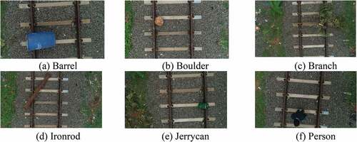
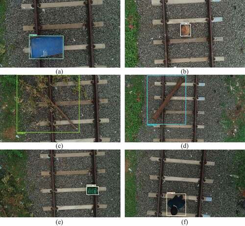
The study area is Tiruchirapalli Junction Railway Station in Tiruchirapalli of Tamil Nadu in India, as shown in Figure 1. The elevation of the railway station spans 95 m with eight platforms and 13 tracks. Among these tracks, a new way was used for data collection. The rail track field was set up with considering various obstacles such as a boulder, iron rod, branch, barrel, person, and jerry can (Figure 2) for aerial railroad obstacle detection. As per guidelines released by Directorate General of Civil Aviation (DGCA) for operating drones in India (Ananth Padmanabhan 2017). The major requirements for the use of UAV in railway environment are initially a licensed remote pilot is appointed for collecting the dataset who has unique identification number from DGCA for operating in the railroad surroundings. After that, obtain permission from division of Indian railways where the datasets are need to be collected. Since the chosen UAV comes under the category of Micro type, it is set to function within the visual line of sight (VLOS).

Figure 1. Location map of the study area ((A) India, (B) Tamil Nadu, (C) Tiruchirapalli, and (D) Railroad Aerial Monitoring for Data Collection).

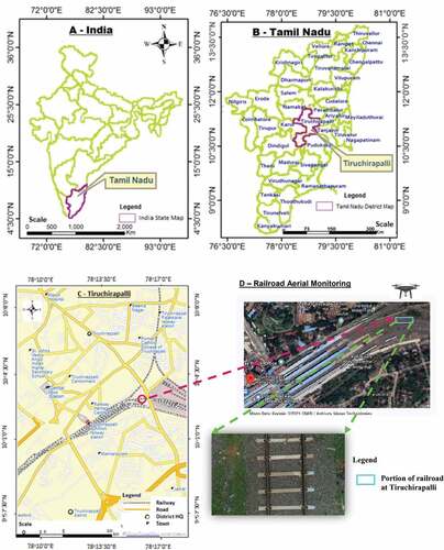
Figure 2. Sample obstacle railroad aerial images in the RODD used to validate diverse deep neural network models where (a)–(f) represents classes used in this study.

The DJI Phantom 4 PRO UAV is furnished with a Sony DSC-RX1RM2 camera, a 20 M (megapixel) full resolution camera used for data collection. The focal length and video recording mode were 8.8 mm and 1920 × 1080 full high definition at 65 Mbps. The aerial videos are collected based on the parameter settings, and the flight path was remotely controlled from the ground station. The total length of the railroad structure in the study area is 500 m. Since it is a low-altitude based aerial railroad obstacle detection processing, the flying altitude was fixed as 10.5 m. Altitude was assigned based on the specifications of Research Design and Standards Organization (RDSO, 2003), India in which the normal height of overhead line from rail level is 5.55 m. The date of the data collection shoot was September 15, 2020, and the video file format was.mov. After collecting the aerial videos, it was uploaded to the IBM Cloud annotation tool (Oliveira et al. 2016) for converting it into frames with.jpg image format and downloaded a total of 315 required images with obstacles. Once all the videos are converted into structures, those images are maintained as a RODD dataset (Railroad Obstacle Detection Dataset). However, In general some limitations such as security hazards, hard to collect data during cyclone, flood, etc. should be considered during data acquisition using UAV.

Data Preprocessing

This phase comprises two steps: data augmentation and data annotation. Since the initial dataset is minimal for training and testing, data augmentation is implemented to avoid overfitting and enhance the performance of the deep neural network models.

The build dataset of 315 images was expanded to six times of original size via various geometric transformations processes, a total of 2002 images. From Keras library, ImageDataGenerator class is used for implementing data augmentation (Aiman Soliman and Jeffrey Terstriep, 2019), which comprises various arguments such as rotation (40, 60), shear (0.2), zoom (0.2), brightness (0.5, 1.5) and horizontal flip. Through the mentioned operation, RODD was created with 80% corresponding to 1602 aerial images are acquired for training and 20% of 400 aerial images for testing.

The next step of augmentation is data annotation using the LabelImg tool used for bounding box creation and labeling. To define the location of the target obstacles bounding box is need to be created (Z-Q Zhao et al. 2018) with six different labellings such as barrel, boulder, person, iron rod, branch and jerrycan. To provide suitable training and testing files for the detectors, two formats of the bounding box are created one is pascal_voc, and another is yolo. Consequently, TensorFlow records and label map files are generated for training the latest tensor flow two object detection models, which is discussed under section 2.3.

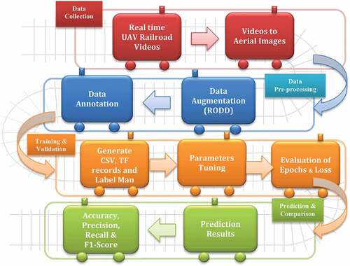
In terms of calculation, training the deep neural network models in this study are intensive. All the configurations are done under anaconda prompt, and the various model training in our study was completed in Colab Pro for implementing railroad obstacle detection. Further, the attained inference graph is used for testing the images using Jupyter Notebook. Since the training was done on Colab Pro, its configuration was set as Tesla 4 GPU and 25 GB RAM. Except for YOLOv3, the other models are chosen from the latest TensorFlow 2 detection model zoo (Selahattin Akkas, Singh Maini, and Qiu 2019). The pipeline of this study comprises four main tasks: dataset collection, pre-processing, training, validation, prediction, and comparison among the deep network models (Figure 3).

Figure 3. Pipeline of assessment on low altitude UAV-based railroad obstacle detection using deep neural network models.

Deep Neural Network Models

Convolutional Neural Network (CNN) is the most commonly used network amongst the deep neural network structures (Kaster, Patrick, and Clouse 2017). CNN comprises of multi-layered architecture where each layer executes its own function and passes the resultant data to the next layer. Multi-layered structure has multilayered deep neural network with back propagation for training usage.

The main two stages involved in CNN are feature extraction and classification in which layers such as input layer, convolution layer, activation function and pooling fall under the taxonomy of feature extraction subsequently fully connected layer, drop out and classification layer fall under the taxonomy of classification (Ghiasi, Lin, and Le 2018). We have evaluated the performance of the four familiar CNN frameworks such as CenterNet, SSD, Faster RCNN and YOLOv3. Further SSD model is used as an object detection algorithm with three backbone models such as EfficientDet, MobileNet and ResNet50 with various input sizes. As a whole, in this study, nine deep neural network models are evaluated (Table 1) for obstacle detection on low-altitude aerial railroad images at high resolution. These deep neural network models were chosen as an outcome of the literature review accomplished subject to the input size, number of parameters and depth. Especially, SSD is a rapid real-time single-shot object detector for multiple classes and considerably more accurate (Liu et al. 2016).

Table 1. Properties of deep neural networks used in this study

Sl. no.	Type	Object detection algorithm	Backbone (feature extraction)	Input size	Parameters (millions)	Depth (#layers)
1.	1-stage	CenterNet	Hourglass104	512 × 512	4.80	104
2.	1-stage	SSD	EfficientDet-d0	512 × 512	3.9	3
			EfficientDet-d1	640 × 640	6.6	3
			EfficientDet-d2	768 × 768	8.1	3
3.	1-stage	SSD	MobileNetv1-FPN	640 × 640	4.24	28
			MobileNetv2	320 × 320	3.47	53
4.	1-stage	SSD	ResNet50	640 × 640	25.5	50
5.	1-stage	DarkNet-53	YOLO v3	608 × 608	59	106
6.	2-stage	Faster RCNN	ResNet50	640 × 640	25.6	50

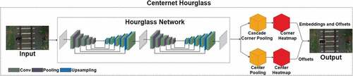
CenterNet Hourglass

CenterNet identifies objects utilizing a triplet, including one keypoint and two corners (Dual et al., 2019). Thus, it models any entity using the center point of the bounding box with the aid of keypoint estimation and reverts to properties like localization, orientation, even poses and size. Hourglass Network module is vast but produces the top keypoint estimation performance. Hourglass network looks like a stack in which it downsamples the input by four multipliers, subsequently by two series of hourglass modules, as shown in Figure 4.

Figure 4. Design of deep neural network model of CenterNet Hourglass.

In this model, the size of bounding box can be fixed adaptively through Equation (1)(1) $\left\{\begin{array}{c}{ }_{MT{L}_x=\frac{(p+1)T{L}_x+(p-1)B{R}_x}{2p}}\\ { }_{MT{L}_y=\frac{(p+1)T{L}_y+(p-1)B{R}_y}{2p}}\\ { }_{MT{L}_x=\frac{(p-1)T{L}_x+(p+1)B{R}_x}{2p}}\\ { }_{MT{L}_y=\frac{(p-1)T{L}_y+(p+1)B{R}_y}{2p}}\end{array}\right.$(1) where ($T{L}_x$, $T{L}_y$) and ($B{R}_x$, $B{R}_y$) represents coordinates of top left corner of pixel i and coordinates of bottom left corner of pixel i respectively. Let j be the middle region of bounding box in which ($MT{L}_x$, $MT{L}_y$) represents coordinates of top left corner of middle region j and ($MB{R}_x$, $MB{R}_y$) represents coordinates of bottom right corner of middle region j.

(1) $\left\{\begin{array}{c}{ }_{MT{L}_x=\frac{(p+1)T{L}_x+(p-1)B{R}_x}{2p}}\\ { }_{MT{L}_y=\frac{(p+1)T{L}_y+(p-1)B{R}_y}{2p}}\\ { }_{MT{L}_x=\frac{(p-1)T{L}_x+(p+1)B{R}_x}{2p}}\\ { }_{MT{L}_y=\frac{(p-1)T{L}_y+(p+1)B{R}_y}{2p}}\end{array}\right.$(1)

where p is odd value used to find the scale of the middle region j.

A Hougleass104 backbone network applies to the cascade corner pooling and center pooling to outcome two center keypoint heatmaps and corner heatmaps, respectively. The abounding box is detected via embedding and offsets. In CenterNet modules, center pooling finds the maximum value of feature maps’ vertical and horizontal directions that detect rich and best recognizable visual patterns. In contrast, corner pooling determines the top deals on the boundary directions of feature maps to find corners that overcome corners at external objects. Heatmap denotes keypoints location and allocates score. Embedding finds whether corners are from similar things and offsets realize to map the corners again from its heatmap to input. Reddy Pailla, Kollerathu, and Chennamsetty (2019) carried out CenterNet Hourglass 104 implementation for object detection on low-resolution and noisy aerial images and achieved better accuracy compared to YOLOv3.

SSD EfficientDet

SSD (Single Shot Multibox Detector) is aimed at real-time object detection. A significant characteristic of this network is the utilization of multiscale convolution layers attached with feature maps produced by the backbone network model. It results in integrated detection of bounding boxes and confidence score of existence labels in those boxes; subsequently, a non-max suppression is used to generate the resultant object detection. An enhanced SSD was implemented on UAV based object detection in the railway scene for providing security (Yundong et al. 2020).

VGG16 (Visual Geometry Group) is the backbone model of original SSD but its author said other neural network model can also be utilized as a backbone network. Recently, compared to VGG16 many other deep neural network models have been achieved better performance. Since this paper concentrates on real-time railroad obstacle detection, accuracy and prediction time is concerned more. Based on this context, three models such as EfficientDet, MobileNet and ResNet50 were executed as its backbone models (Figure 5) and the detail are given in the later subsections.

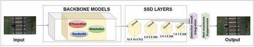
Figure 5. Design of deep neural network model of SSD.

EfficientDet is a deep neural network for object detection offered by Google (Tan, Pang, and Le 2020); which comprises of feature extraction network, i.e. EfficientNet (Tan and Le 2019), a weighted bi-directional feature pyramid network (BiFPN), depth and image resolution of any model, compound scaling technique that improves performance through scaling width, and prediction network for identifying bounding boxes. In this study, EfficientDet is implemented as a backbone model, whereas SSD layers are used for railroad obstacle detection (Figure 6).

Figure 6. Design of deep neural network model of SSD EfficientDet.

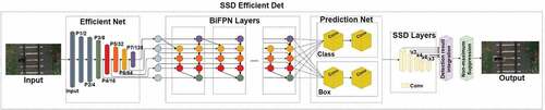
BiFPN considers P3 to P7 features from the efficient net and repetitively operates bottom-up and top-down multifeature fusion in this network. Significant levels involved in BiFPN is the fusion of fast-normalized fusion and bidirectional cross connections which is defined in the Equation (2)(2) $P_5^{out}=Conv\left(\frac{{w_1}^{\prime }.P_5^{in}+{w_2}^{\prime }.P_6^{in}+{w_3}^{\prime }.Resize\left(P_4^{out}\right)}{{w_1}^{\prime }+{w_2}^{\prime }+{w_3}^{\prime }+\epsilon }\right)$(2) :

(2) $P_5^{out}=Conv\left(\frac{{w_1}^{\prime }.P_5^{in}+{w_2}^{\prime }.P_6^{in}+{w_3}^{\prime }.Resize\left(P_4^{out}\right)}{{w_1}^{\prime }+{w_2}^{\prime }+{w_3}^{\prime }+\epsilon }\right)$(2)

Where $wi$≥ 0 is weight, =0.0001 is a minor value to prevent numerical variation, Conv is a convolutional operation for generating feature maps and Resize is either upsampling or down sampling process for resolution matching. Bounding Box model depth (channel) and width can be calculated using the following Equation (3)(3) $D_{box\mathrm{\_}pred}=3+\left(\frac{\mathrm{\varnothing }}{3}\right),W_{box\mathrm{\_}pred}=64\times \left({1.35}^{\mathrm{\varnothing }}\right)$(3) :

(3) $D_{box\mathrm{\_}pred}=3+\left(\frac{\mathrm{\varnothing }}{3}\right),W_{box\mathrm{\_}pred}=64\times \left({1.35}^{\mathrm{\varnothing }}\right)$(3)

Where $\mathrm{\varnothing }=0to2\mathrm{i}\mathrm{n}$ this study which represents levels of the model. After that, these features are passed to the box/class net for generating bounding box and object class predictions. EfficientDet achieves fewer parameters compared to other state-of-art algorithms with better accuracy and efficiency. It is a family of deep neural network models (from d0 to d7) showing a similar structure at various model size scales. In the context of this study, four EfficientDet models (D0, D1, and D2) with varying input sizes were implemented for low-altitude railroad obstacle detection.

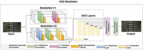
SSD MobileNet

MobileNet is a deep neural network that utilizes depthwise separable convolutions to construct a lightweight deep learning model (Howard et al. 2017). Depthwise separable convolutions lead to nine times lesser amount of work compared to other neural networks with equal accuracy. In this study, MobileNet V1 and MobileNet V2 are implemented as backbone along with SSD object detection algorithm. In MobileNet V1, the depthwise separable convolution layer is divided into depthwise convolution and 1 × 1 pointwise convolution. After each convolution layer, batch normalization and relu6 are treated, followed by the global average pooling layer and the complete connected classification layer are processed (Figure 7).

Figure 7. Design of deep neural network model of SSD MobileNet.

Equation 4(4) $O_{f,k,n}=\sum _{i,j}{F}_{i,j,n}\times K_{f+i-1,j-k,n}$(4) defines a filter used for feature processing as per input depth (channel) involved in depthwise convolution. Nth channel of filtered output feature O is produced by nth kernel in F is applied to the nth depth in K.

(4) $O_{f,k,n}=\sum _{i,j}{F}_{i,j,n}\times K_{f+i-1,j-k,n}$(4)

where F is the depthwise convolution filter of size D_F×D_F×N in which D_F represents filter size supposed to be square and N denotes number of input depths.

On the other hand, in MobileNet V2 (Sandler et al. 2018) has an expansion layer, depthwise convolution layer and projection layer executed under residual connection. In version 1, the pointwise convolution layer retained the same number of layers or doubled it. In contrast, in version 2, with the execution of the projection layer, the number of channels size get lesser. In (Suharto et al. 2020), SSDMobileNet V1 is executed for detecting types of fish with better accuracy rate, and in (Chiu et al. 2020), MobileNet-SSD V2 is implemented for object detection with better performance.

SSD ResNet50

Residual Networks with 50 Layers (ResNet50) hold the idea of skipping blocks of convolution layers using skip connections (He et al., 2017). The ultimate aim of deep neural networks is to learn deeper features to resolve complex tasks with high accuracy and speed. Of course, while training, all the layers learn high or low-level features, but in the residual network, the model learns residual. In residual block, input x is added as a residue with the outcome of weight layers, and Relu activation is carried out in between these layers. Building block of residual network can be defined using the Equation 5(5) $O=F\left(I,\left\{W_i\right\}\right)+I$(5) :

(5) $O=F\left(I,\left\{W_i\right\}\right)+I$(5)

Where I and O are the input and output values of the considered layers. W_i denotes weight carry at each process and the function $F\left(I,\left\{W_i\right\}\right)$ denotes the feature mapping to be learned at residual process.

In this study, SSD with ResNet 50 v1 (also known as RetinaNet) is used for railroad obstacle detection trained on COCO dataset with input images for training scaled to 640 × 640 (Figure 8, Figure 9). There are three structures associated with residual network i.e., with layers of 50, 101 and 152. The reason is to choose resnet50 for this study, computational complexity of resnet 152 is 3.1 times larger than resnet 50 and also the top five accuracy rate varies only by 0.7%. Henceforth, ResNet50 is used as backbone model for SSD obstacle-detection algorithm.

Figure 8. Design of deep neural network model of SSD ResNet50.

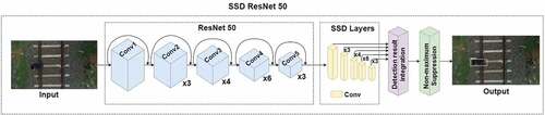
Figure 9. Design of deep neural network model of YOLOv3.

YOLOV3

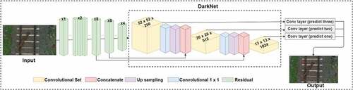
This is one of the most familiar models of object detection techniques. The reason is that it applies for only one forward pass on the whole image and predicts bounding boxes and class probabilities. Internally, YOLO (You Only Look Once) is divided into feature extraction and feature detection (Redmon and Farhadi 2018). The difference in the previous versions of YOLO can be noted in the Feature Extraction part and accomplishes significant outcomes, especially on low-altitude aerial datasets. Here, the improvisation is made by combining the processes of YOLO V3 and Darknet-53. Equation 6(6) $\begin{array}{rl}& b{b}_i=\epsilon \left(o_i\right)+t{l}_i\\ & b{b}_j=\epsilon \left(o_j\right)+t{l}_j\\ & b{b}_w=a_w.e^{o_w}\\ & b{b}_h=a_h.e^{o_h}\end{array}$(6) defines the prediction of bounding box in image using YOLOv3 model.

(6) $\begin{array}{rl}& b{b}_i=\epsilon \left(o_i\right)+t{l}_i\\ & b{b}_j=\epsilon \left(o_j\right)+t{l}_j\\ & b{b}_w=a_w.e^{o_w}\\ & b{b}_h=a_h.e^{o_h}\end{array}$(6)

Where, $b{b}_i,b{b}_j,b{b}_w,b{b}_h$ are the center coordinates, width and height of the prediction results. tl and tl are the top left coordinates. o_i,o_j,o_w,o_h are the output of the model and $a_{w}and{a}_h$ denotes bounding box anchor dimension.

Darknet-53 is nothing but the number of layers present in which is 53. These layers are stacked with the detection head consisting of another 53 layers, which sums up to 106 layers – the overall fully convolutional layers present. The Feature Detector will put in 1 × 1 kernel on feature maps of three diverse sizes at three various locations. In (Tan, Pang, and Le 2020), UAV-YOLO was proposed for object detection on low altitude aerial images where darknet structure is improvised by adding few convolution layers at the early channels, which enriches spatial information.

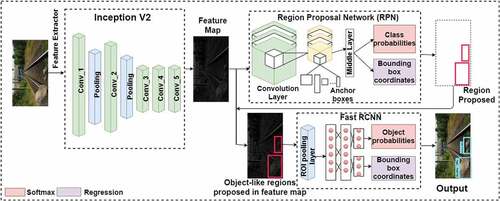
FasterRCNN

Faster RCNN (Faster Region-based Convolutional Neural Network) combines two modules: Fast RCNN, a detector, and RPN that gives the region proposals (Ren et al., 2015). Images taken as input for the model are passed through the convolutional networks that produce the feature maps from each image. Then the Region Proposal Network (RPN) is put over the established feature maps and got the object proposals. Also, the RPN generates the anchors for the given input image and ranks them based on the probability that it contains an object.

The RoI (Region of Interest) pooling layer brings all the object proposals obtained from the previous layer to the same size. It is moved to a fully connected layer that finally classifies and predicts the resultant bounding boxes for the image given as input. In Faster RCNN, bounding box regression loss $(L_{loc})$ for image can be computed as summation of all foreground anchors regression losses $\left(L_k\right)$ which is defined in Equation 7(7) $L_{lo}=\sum _{\begin{array}{c}k\in all\\ foreground\\ anchors\end{array}}{L}_k$(7) :

(7) $L_{lo}=\sum _{\begin{array}{c}k\in all\\ foreground\\ anchors\end{array}}{L}_k$(7)

where,

(8) $L_k=\sum _{\hspace{0.17em}}x\in w,h,i,jsmoot{h}_{L1}(k_x^{predicted}-k_x^{target})$(8)

(9) $smoot{h}_{L1}\left(x\right)=\left\{\begin{array}{c}\frac{{\epsilon }^2{x}^2}{2}\left|i\right|<\frac{1}{{\epsilon }^2}\\ \left|i\right|-\frac{0.5}{{\epsilon }^2}else\end{array}\right.$(9)

The above Equation 8(8) $L_k=\sum _{\hspace{0.17em}}x\in w,h,i,jsmoot{h}_{L1}(k_x^{predicted}-k_x^{target})$(8) illustrates foreground anchor loss calculated by subtracting predicted and target coefficients in which w, h, i, and j denotes width of box, height of box and coordinates of top left corner respectively. Equation 9(9) $smoot{h}_{L1}\left(x\right)=\left\{\begin{array}{c}\frac{{\epsilon }^2{x}^2}{2}\left|i\right|<\frac{1}{{\epsilon }^2}\\ \left|i\right|-\frac{0.5}{{\epsilon }^2}else\end{array}\right.$(9) defines smooth L1 loss which is mostly used as loss function in the models implemented in this study where ε is selected as arbitrarily. Some interesting Faster RCNN implementations are available (Li et al. 2018). It was applied for low-resolution aerial images and detecting birds through super and very super resolution CNN techniques. ResNet50 is a backbone model in this study, whereas FasterRCNN is used for railroad obstacle detection (Figure 10).

Figure 10. Design of deep neural network model of FasterRCNN.

Table 2 illustrates the hyper-training parameters of various deep neural network models used in this study. Learning rate was chosen as 1e-3 for centernet as well as yolov3 and 8e-3 for other models; likewise, momentum was set as 0.9 to all models. The batch size is assigned as two that refer to the number of sample data transmitted throughout the network model. Advantage of using mini-batch size requires less memory and train faster. Steps hold a value that describes how many numbers of steps need to be completed in a series order to create a model checkpoint for exporting inference. Optimizers are used to reduce the losses and maximize the efficiency of the outcome by changing the properties of models, such as learning rate and weight. All models used momentum optimizer except centernet that used Adaptive Moment Estimation (Adam) optimizer. Due to variation in loss and accuracy with epochs, the optimizers were chosen for each model. Decay (weight decay) is mainly used to prevent the weights from increasing too large, so after each update, the weights are multiplied by 0.99. The warmup learning rate is .0001, which defines the maximum reach of the learning rate afore beginning to drop.

Table 2. Training hyper parameters of deep neural network models

Parameters/ models	CenterNet Hourglass	SSD EfficientDet (D0, D1, D2)	Faster RCNN	SSD MobileNet (V1, V2)	SSD ResNet50	YOLOv3
Learning Rate	1e-3	8e-3	8e-3	8e-3	8e-3	1e-3
Batch Size	2	2	2	2	2	2
No. of Steps	12000	10000	25000	25000	25000	10800
Momentum	0.9	0.9	0.9	0.9	0.9	0.9
Optimizer	Adam	Momentum	Momentum	Momentum	Momentum	SGD with Momentum
Activation	Relu	Swish	Relu	Relu6	Relu6	Leaky
Warmup learning rate	.0001	.0001	.0001	.0001	.0001	.0001
Decay	0.99	0.99	0.99	0.997	0.997	0.0005
Classification Loss	Focal loss	Weighted sigmoid focal	Log loss	Weighted sigmoid focal	Weighted sigmoid focal	Binary Cross Entropy
Localization Loss	L1 Localization	Weighted smooth L1	Weighted smooth L1	Weighted smooth L1	Weighted smooth L1	Sum of squared error
Score threshold	0.2	0.2	0.1	1e-8	1e-8	0.7
IoU threshold	0.5	0.5	0.6	0.6	0.6	0.9

The overall loss function is a weighted sum of classification loss and localization loss, where classification loss is the loss in naming class labels to predicted bounding boxes, and localization loss identifies the gap between the ground truth boundary box and predicts boundary box. Additionally, smooth L1 loss is inferior for accurate obstacle localization. At first, the image is divided into a grid of cells and finds the grid cell that has the center of the image, and for that grid, it predicts the bounding boxes and class probabilities of classes to which it belongs. Then, the results of each probability of all the possible classes in the object are aggregated using Non-Maximum Suppression (NMS) based on the threshold of the objects such as score and you. This threshold is nothing but set the minimum confidence score that is acceptable for detection.

Algorithm

The algorithm for training and evaluating aerial railroad images for obstacle detection using deep neural network models is presented as follows:

Algorithm 1 Obstacle Detection – Training and Evaluation on Aerial Railroad Images

Input: Aerial railroad images

Output: Dangerous railroad obstacle detection results

1: Data Augmentation ← Expand the images by ImageDataGenerator Class

2: RODD dataset ← Data annotation through bounding box creation and labeling

3: Train and Test images ← Split the total images (original + augmented) in the ratio of 80:20

4: Generated CSV file ← From training and testing images

5: Generated TFrecord files ← From csv file, classes file, training and testing images

6: Generated Labelmap ← Create id and name for each class as an item

7: Parameter Adjustments ← Fine tune arguments of model configuration file

8: Trained model ← Input pipeline configuration file into model

9: Evaluated training model ← mAP, AR, classification loss, localization loss and total loss

9: Export inference graph ← After successful completion of training

10: Railroad obstacle detection results ← Input the test images with obstacles into the trained model

11: Evaluate the railroad obstacle detection results ← Classification metrics such as TP, FP, TN, FN, Pr, Rc, F1-Score, Acc, IoU and DC

Evaluation Metrics

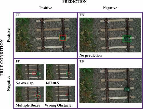
Four combinations of values are computed to measure the performance of a deep neural network model in predicted classes of test data with actual classes. This evaluation is based upon the computation of the confusion matrix of six classes for all the deep neural network models considered in this study. The confusion matrix is a table that defines the performance of the railroad obstacle detection model on test data where all four values are identified.

The values are True Positive (TP), True Negative (TN), False Positive (FP), and False Negative (FN). TP value signifies the number of correctly detected obstacles on the railroad. FP value represents the number of wrongly detected obstacles in the railroad. FN value mentions the number of missing obstacles or undetected obstacles by the detection model. TN value refers to the number of nonobstacles that are correctly identified as nonobstacles. Additionally, Precision (Pr), Recall (Rc), F1-Score (F1), and Accuracy (Acc) are obtained from the confusion matrix and calculated as follows (Equation 10(10) $Precision(Pr)=\frac{TP}{TP+FP}$(10) to Equation 13)(13) $Accuracy(Acc)=\frac{TP+TN}{TP+FP+FN+TN}$(13) :

(10) $Precision(Pr)=\frac{TP}{TP+FP}$(10)

(11) $Recall(Rc)=\frac{TP}{TP+FN}$(11)

(12) $F1-Score(F1)=\frac{2\times Precision\times Recall}{Precision+Recall}$(12)

(13) $Accuracy(Acc)=\frac{TP+TN}{TP+FP+FN+TN}$(13)

The other performance metrics considered in this study for calculating the accuracy of an obstacle detector on RODD are Intersection over Union (IoU) and Dice Coefficient (DC). The predicted bounding box can be evaluated using IoU as the ratio of the overlapping area and predicted area to the complete area. The IoU is between 1 (perfect overlap) and 0 (no overlap) (Breton 2019). Nevertheless, in railroad obstacle detection task, IoU could be defined as follows: (Equation 14(14) $IoU(GTB,PBB)=\frac{\alpha \left|BGT\cap BBP\right|}{\alpha \left|BGT\cup BBP\right|}=\frac{TP}{TP+FP+FN}$(14) )

(14) $IoU(GTB,PBB)=\frac{\alpha \left|BGT\cap BBP\right|}{\alpha \left|BGT\cup BBP\right|}=\frac{TP}{TP+FP+FN}$(14)

Where α is the set counting quantity, i.e. area, GTB denotes bounding box of ground truth and BBP represents bounding box of prediction.

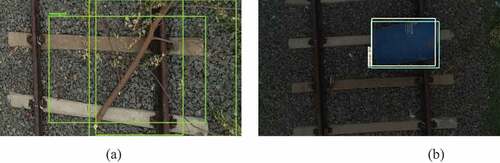
The following are the rules applied to each aerial railway image to calculate the IoU: (1) TP: BBP associated to BGT has an IoU greater than threshold (2) FN: No match in BGT (3) IoU between BBP and BGT is less than threshold and (4) TN: No BGT and BBP. This is illustrated in Figure 11. Also it is characterized the deep learning models with various threshold values such as 0.5, 0.6, and 0.9. The IoU threshold values of the considered deep learning models are given in Table 2.

(15) $DiceCoefficient(DC)=\frac{2TP}{2TP+FP+FN}$(15)

Figure 11. Illustration of IoU metric in which BBGT are colored in green and BBP are colored in red.

DC is used to find how similar the obstacles are from actual to predicted image, i.e. it is an overlap-based metric between the actual image and predicted image. If the overlap region is similar to the union region, it leads to correct classification and comes under the concept of f1-score. DC is defined in Equation 15(15) $DiceCoefficient(DC)=\frac{2TP}{2TP+FP+FN}$(15) .

Results and Analysis

In this study, the experimental results evaluated the real-time obstacle detection on aerial railroad images using nine deep neural network models. The training was implemented through nine different models on a total of 2002 images in the Real Obstacle Detection Dataset (RODD). According to the best practices of object detection models and cross-validation principle (ML Crash Course at Google, 2020), the training and testing dataset is split up as 80–20 among the total dataset (Li, Zhao, and Zhou 2019). Especially in the RODD, 1602 labeled images are in the training folder, and 400 images are in the test folder. Table 3 illustrates the quantitative evaluation metrics discussed in section 2.5 for training the model for railroad obstacle detection of various models.

Table 3. Comparison of outcomes using various assessment metrics

Sl. no.	Model	Pr (%)	Rc (%)	F1 (%)	Ac (%)	IoU(%)	DC(%)	Time(s)
1	CenterNet Hourglass104	72.46	75.75	71.31	72.00	56.82	71.24	10800
2	SSD EfficientDet D0	82.51	83.77	82.79	82.75	70.82	82.79	7200
3	SSD EfficientDet D1	75.37	73.19	70.88	71.75	45.72	58.88	7200
4	SSD EfficientDet D2	76.79	78.55	76.67	77.25	62.93	76.67	7200
5	FasterRCNN	85.16	83.61	80.39	84.75	72.27	83.04	10800
6	SSD MobileNet V1	87.67	85.40	85.55	86.50	75.07	85.55	7200
7	SSD MobileNet V2	95.89	97.22	96.41	96.75	93.18	96.41	10800
8	SSD ResNet50	83.56	84.52	83.66	83.75	72.05	83.66	10800
9	YOLOv3	70.68	73.64	70.88	70.83	55.79	70.87	14400

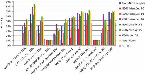
Based on the table, the SSD MobileNet model produced a greater success ratio, especially SSD MobileNet V2 with input size 320 × 320. On the other side, YOLOv3 generated lower accuracy compared with other models. SSD MobileNet V2 model precision was computed as 95.89%, recall as 97.22%, f1-score as 96.41%, accuracy as 96.75%, intersection over union as 93.18 and dice coefficient as 96.41%. Particularly accuracy were acquired as 72% (CenterNet Hourglass), 82.75% (SSD EfficientDet d0), 71.75% (SSD EfficientDet d1), 77.25% (SSD EfficientDet d2), 84.75% (Faster RCNN), 86.50% (SSD Mobilenet v1), 96.75% (SSD MobileNet v2), 83.75% (SSD ResNet50), and 70.83% (YOLOv3).

Figure 12 shows the confusion matrices of all deep neural network models in this study, representing the accuracy of railroad obstacle detection of individual classes. In this study, six classes, such as barrel, boulder, branch, iron rod, jerry can, and the person, is considered and evaluated through a confusion matrix. The values in confusion matrices represent the four combinations of values such as TP, FP, FP, and TN, which are used for calculating precision, recall, f1-score, accuracy, intersection over union, and dice coefficient. SSD MobileNet V2 scores high TP values in the railroad obstacle detection represented as green color code among all models. For instance, considering a class barrel in YOLOv3 in which its TP value is scored as 18, FP value is scored as 9 (3 + 2 + 1 + 3), FN value is one, and TN value is 67 (11 + 9 + 15 + 17 + 15). It means 18 barrel obstacles are correctly identified from the RODD dataset, 9 barrel obstacles are wrongly detected on the railroad, 1 barrel obstacle is not detected by this model, and 67 obstacles other than barrel are correctly identified as its respective railroad obstacle classes.

Figure 12. Confusion Matrices of various deep neural network models used in this study where SSD MobileNet V2 scores high TP values in railroad obstacle detection, represented as green color code.

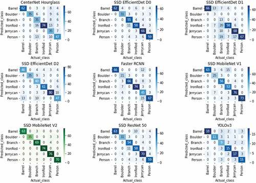
Similarly, for all the classes, combinations of values are calculated. In this, YOLOv3 scores very few TP values and more FP values for each class. That is why its accuracy value is significantly less compared to other models. The high accuracy scorer SSD MobileNet V2 has more TP values and fewer FP values for an individual class. Thus, scoring more TP values and less FP, FN values lead to better accuracy of the railroad obstacle detection model. Table 4 illustrates metric values such as Pr, Rc, F1, IoU, DC, Acc, macro average, and weighted average of assessment on various classes to identify the best deep neural network model for railroad obstacle detection.

Table 4. Assessment on various classes using metrics for identifying best deep neural network model for railroad obstacle detection

Models	CenterNet Hourglass 104					SSD EfficientDet D0					SSD EfficientDet D1
Classes/Metrics	Pr (%)	Rc (%)	F1 (%)	IoU (%)	DC (%)	Pr(%)	Rc (%)	F1 (%)	IoU (%)	DC (%)	Pr (%)	Rc (%)	F1 (%)	IoU (%)	DC (%)
Barrel	80.52	100.00	89.21	80.52	89.21	81.58	100.00	89.86	81.58	89.86	71.74	100.00	83.54	71.39	83.54
Boulder	62.50	100.00	76.92	62.50	76.92	77.50	88.57	82.67	70.45	82.67	100.00	10.34	18.75	10.34	18.75
Branch	71.43	47.95	57.77	40.23	57.38	87.30	75.34	80.88	67.90	80.88	76.47	18.84	30.23	17.81	30.23
IronRod	69.81	100.00	82.22	69.81	82.22	76.32	78.38	77.33	63.04	77.33	63.74	78.38	70.30	54.21	70.30
Jerrycan	83.33	42.17	56.00	38.89	56.00	90.41	79.52	84.62	73.33	84.62	80.95	71.58	75.98	61.26	75.98
Person	67.14	64.38	65.74	48.96	65.73	81.94	80.82	81.38	68.60	81.38	59.29	100.00	74.44	59.29	74.44
Accuracy	72.00	72.00	72.00	72.00	72.00	82.75	82.75	82.75	82.75	82.75	68.75	68.75	68.75	68.75	68.75
Macro Avg	72.46	75.75	71.24	56.82	71.24	82.51	83.77	82.79	70.82	82.79	75.37	63.19	58.88	45.72	58.88
Weighted Avg	73.45	72.00	69.86	73.45	69.86	83.19	82.75	82.64	83.19	82.75	73.23	68.75	63.88	73.20	63.88
Models SSD EfficientDet D2						FasterRCNN ResNet50					SSD MobileNet V1
Classes/Metrics	Pr (%)	Rc (%)	F1 (%)	IoU (%)	DC (%)	Pr (%)	Rc (%)	F1 (%)	IoU (%)	DC (%)	Pr (%)	Rc (%)	F1 (%)	IoU (%)	DC (%)
Barrel	75.41	69.70	72.44	56.79	72.44	84.62	100.00	91.67	84.62	91.67	72.41	100.00	84.00	72.41	84.00
Boulder	68.63	100.00	81.40	68.63	81.40	87.50	60.00	71.19	55.26	71.19	89.29	71.43	79.37	65.79	79.37
Branch	81.63	57.97	67.80	51.28	67.80	82.50	95.65	88.59	79.52	88.59	93.33	77.78	84.85	73.68	84.85
IronRod	87.14	82.43	84.72	73.49	84.72	88.10	100.00	93.67	88.10	93.67	94.64	71.62	81.54	68.83	81.54
Jerrycan	80.81	96.39	87.91	78.43	87.91	86.54	54.22	66.67	50.00	66.67	88.37	91.57	89.94	81.72	89.94
Person	67.14	64.84	65.73	48.96	65.73	81.71	91.78	86.45	76.14	86.45	87.95	100.00	93.59	87.95	93.59
Accuracy	77.25	77.25	77.25	77.25	77.25	84.75	84.75	84.75	84.75	84.75	86.50	86.50	86.50	86.50	86.50
Macro Avg	76.79	78.48	76.67	62.93	76.67	85.16	83.61	83.04	72.27	83.04	87.67	85.40	85.55	75.07	85.55
Weighted Avg	77.67	77.25	76.68	77.67	76.68	85.02	84.75	83.58	85.02	83.58	87.92	86.50	86.27	87.92	86.27
ModelsSSD MobileNet V2						SSD ResNet50					YOLOv3
Classes/Metrics	Pr (%)	Rc (%)	F1 (%)	IoU (%)	DC (%)	Pr (%)	Rc (%)	F1 (%)	IoU (%)	DC (%)	Pr (%)	Rc (%)	F1 (%)	IoU (%)	DC (%)
Barrel	95.45	100.00	97.67	95.45	97.67	81.82	100.00	90.00	81.82	90.00	66.67	94.74	78.26	64.29	78.26
Boulder	85.37	100.00	92.11	85.37	92.11	77.50	88.57	82.67	70.45	82.67	68.75	100.00	81.48	68.75	81.45
Branch	94.52	95.83	95.17	90.79	95.17	93.10	75.00	83.08	71.05	83.08	60.00	42.86	50.00	33.33	50.00
IronRod	100.00	100.00	100.00	100.00	100.00	80.56	78.38	79.45	65.91	79.45	83.33	68.18	75.00	60.00	75.00
Jerrycan	100.00	91.57	95.60	91.57	95.60	86.42	84.34	85.37	74.47	85.37	73.91	70.83	72.34	56.67	72.34
Person	100.00	95.89	97.90	95.89	97.90	81.94	80.82	81.38	68.60	81.38	71.43	65.22	68.18	51.72	68.18
Accuracy	96.75	96.75	96.75	96.75	96.75	83.75	83.75	83.75	83.75	83.75	70.83	70.83	70.83	70.83	70.83
Macro Avg	95.89	97.22	96.41	93.18	96.41	83.56	84.52	83.63	72.05	83.66	70.68	73.64	70.88	55.79	70.87
Weighted Avg	97.02	96.75	96.78	97.02	96.78	84.22	87.50	86.26	84.22	86.26	71.11	70.83	69.90	71.11	69.90

In Table 4, SSD MobileNetV2 holds almost the expected values of all the classes especially class IronRod meets 100% values in all the metrics and achieves a higher accuracy value of 96.75% than other models. Other than the MobileNet model, the next highest metric value reached for all the classes is Faster RCNN. This two-stage detector scores 84.75% accuracy, and all the classes scored accepted reasonable values. Likewise, the least metric values are produced by the model YOLOv3 for all the classes compared to other models with an accuracy of 70.83%. In few classes of the models, when precision scores 100%, its recall value is only 10.34%, and f1-score is 18.75%, reflecting in the value of IoU and DC with the same values.

Mean Average Precision (mAP) is used to evaluate railroad obstacle detection accuracy. On the RODD dataset, the map results of deep neural network models used in this study are shown in Figure 13. The AR (Accuracy Recall) and mAP values in IOU = 0.5 of MobileNet V2 are almost 2% higher than FasterRCNN and nearly 30%–50% higher than YOLOv3. Even further severe test cases under IOU from 0.50 to 0.95 and IOU = 0.75, the mAP and AR values of MobileNet V2 is 2% higher than Faster RCNN and 20%–50% higher than YOLOv3. Practically, MobileNet V2 produces a higher success ratio in terms of mAP and AR when compared to all other models. Figure 8 also specifies that MobileNet V2 needs more improvements in detecting small objects than medium and large objects. In this case, all the models produce very few mAP and AR values. Hence, improvisation is required for detecting small objects by the deep neural network models used in this study.

Figure 13. Performance of mAP on RODD using deep neural network models in this study.

The loss function is used to measure how better the trained deep neural network model is performed in predicting the expected railroad obstacle detection output. It computes the gap between ground truth and predicted outcome, and the optimizers try to reduce the model’s loss value near zero, which gives a better model. The graph of loss function mainly consists of classification loss, localization loss, and total loss of the railroad obstacle detection model considered in this study (Figure 14). In this graph, the x-axis represents some steps taken for calculating loss, and the range of loss values is denoted in the y-axis. For instance, considering the classification loss graph of the SSD MobileNet model (Figure 14 – (d)), loss values range from 0.9 to 0.3.

Figure 14. Classification loss, Localization loss, and Total loss where saffron color denotes training loss against steps and light saffron color represents test loss: (a) CenterNet Hourglass, (b) SSD EfficientDet, (c) Faster RCNN, (d) SSS MobileNet, (e) SSD ResNet50, and (f) YOLOv3.

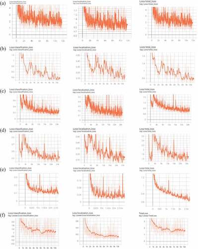
In this graph, in the beginning, the training loss value is 0.3 and suddenly rose beyond the 0.9 loss value. Still, after that, the classification loss graph gradually falls with minor ups that lead to the expected accuracy value. Likewise, localization loss and total loss values exist between 0.5–0.1 and 1.6–0.6, respectively. However, the variation obtained between training and test loss reflects in the YOLOv3 model compared to other models. This may lead it to produce less accuracy value when compared to other models. It is observed that when the loss value touches 0, then the training attainment has been revealed on the test images. Except for CenterNet and YOLOv3, almost all the model’s loss values reaches 0.6, which leads to effective performance.

Since the MobileNet V2 model provided better accuracy than other models, Figure 15 shows railroad obstacle detection using SSD MobileNet V2 with a confidence score. The confidence score is the probability value of the bounding box that covers the obstacle. If the confidence score is less than the threshold, then the obstruction is not detected, and the detection falls on TN. For instance, in the YOLOv3 model, the threshold is set as 30%, so during testing, if the probability value is below 30%, then it is considered TN. In the below figure, obstacle barrel is detected with 71% confidence score, class boulder is seen with 74% confidence score, branch obstacle is found with 78% confidence score, iron rod obstacle is detected with 75% confidence score, obstacle jerrycan is seen with 79% confidence score, and person class is found with 73% confidence score.

Figure 15. Railroad obstacle detection using MobileNetv2: (a) Barrel obstacle detection, (b) Boulder obstacle detection, (c) Branch obstacle detection, (d) IronRod obstacle detection, (e) Jerrycan obstacle detection, and (f) Person obstacle detection.

A robust obstacle detection deep neural network model has to be established for the railroad application in complex environmental situations. One of the major challenges involved in this application is light condition. Four different light illumination effects, such as the original image, are used on images to test the obstacle detection performance during the influence of the light condition. Light effects are original image, light 85%, light 50%, and light 20%. Figure 16 illustrates the testing outputs for the chosen lighting conditions using SSD MobileNet V2.

Figure 16. Railroad obstacle detection results on different light conditions.

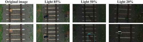
In the above figure, the obstacles are detected under various light conditions such as 85%, 50%, and 20%. Especially, light with 20% column contains jerrycan obstacle. Detecting a small obstacle in a low lighting area is a tedious one as the light value goes lesser and the image’s background turns darker. But in this environmental condition also the model performs well with good accuracy results. These light variations input images were generated using altering the values of the brightness range argument available in the Keras image generator class.

Non-max suppression suppresses the overlapping bounding boxes and displays a single bounding box that scores a high probability value. So to prevent such overfitting outcomes, it is suggested that the initial value of score threshold value 0 can be changed to the minimum value of 0.2, and your threshold can be reduced to a lower value. But even though the bounding box non-max suppression parameters such as score threshold and your threshold is fixed as appropriate in the tensor flow object detection model, Figure 17 (a) represents overlapping bounding boxes in railroad obstacle detection.

Figure 17. (a) Overlapping bounding boxes and (b) misclassification.

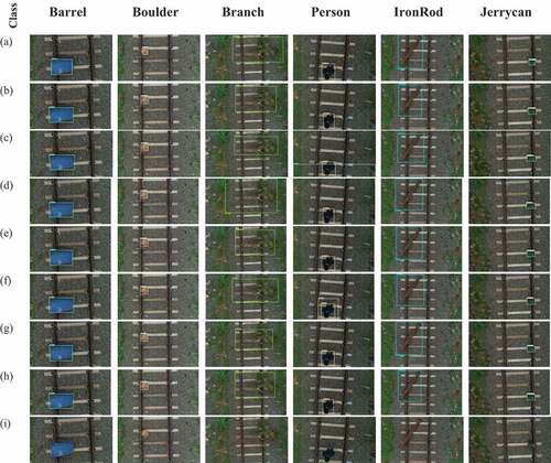
In this case study, non-max suppression parameters of all the models were adjusted to the required value and found that only three models like MobileNet, EfficientDet and YOLOv3, possess this issue. Other than these three models, all other models such as CenterNet Hourglass, Faster RCNN and ResNet50 supported nonmax suppression and produced nonoverlapping bounding boxes for the test images. The worried think is the best model of obstacle detection in this study comes under this issue. But the satisfaction is, it obtained only for few test images of the models. So a highly efficient method is needed for solving this overlapping, especially to the MobileNet models. On the other hand, the misclassification problem is there, which is required to be rectified since it leads to a false positive value and affects the model’s accuracy. Mainly this study considers obstacle detection on railroad aerial images using various deep neural network models. Figure 18 visually outlines some of the railroad obstacle detection on all the six classes using deep neural network models considered in this study. All the test aerial railroad images are acquired from RODD.

Figure 18. Railroad obstacle detection on all the six classes using deep neural network models consider in this study: (a) CenterNet Hourglass 104, (b) SSD EfficientDet d0, (c) SSD EfficientDet d1, (d) SSD EfficientDet d2, (e) Faster RCNN, (f) SSD MobileNet v1, (g) SSD MobileNet v2, (h) SSD ResNet50, and (i) YOLOv3.

Conclusion

Accurate railroad obstacle detection is essential for effective and timely avoidance of accidents like derailments in railways. Existing manual monitoring and sensors mounted on rail or train or somewhere nearby rails lack accuracy in obstacle detection particularly; replacing failure sensors or batteries is very hard at unmanned areas like a dense forest or highly elevated bridges. In this study, real-time UAV based low altitude railroad obstacles monitoring and data source collections were performed and expanded those images using augmentation. After that, annotation was done for creating our own dataset RODD. All set, so the tensor flow object detection models’ configuration was followed by training various deep neural network models such as CenterNet Hourglass, EfficientDet D0, EfficientDet D1, EfficientDet D2, SSD MobileNetV1, SSD MobileNetV2, SSD ResNet50, Faster RCNN, and YOLOv3 was implemented successfully. Lastly, each model and class are assessed with various metrics such as precision, recall, accuracy, intersection over union and dice coefficient, and the influence of light conditions and limitations such as overlapping and misclassifications.

The experimental results illustrate that the models SSD MobileNet V2, Faster RCNN, and SSD ResNet50 performed better than other models with accuracy 96.75%, 84.75%, and 83.75%, respectively, all these models loss values reach 0.6 in that way signifying the success of the training. Since this study was implemented based on the latest tensor flow two object detection models, it took a reasonable time to train the model compared to existing models. It was also perceived that training model time for SSD MobileNet V1, Faster RCNN and SSD ResNet50 are similar. In short, it was understood that the SSD MobileNet V2 is the most appropriate model among the models used for detecting obstacles in the railroad. The obtained outcomes indicated that the latest tensor flow two object detection models could be used for real-time railroad obstacle detection.

The acquired results within the scope of this study illustrated that it is possible to detect the obstacles in the railroad using RODD. To overcome the limitations and increase the models’ performance, more datasets with diversity could be collected or by creating modifications in the deep neural network models. It is also possible to acquire even more effective results by using a high-end system with proper configuration. Additionally, it is believed that this study results and assessments will create necessary support to the related works and also to the researchers researching railroads, implementation of onboard obstacle detection using deep neural network models, fast obstacle detection and give alert to the railway station, obstacle detection at tunnels, etc.

Acknowledgments

The authors would like to thank the Indian Railways, Tiruchirapalli Division, Tamil Nadu, India for giving permission to capture UAV images.

Disclosure statement

No potential conflict of interest was reported by the author(s).

Data Availability Statement

For kind information, the dataset we have created for this research work is going to use for the extended work. During review period, I will share sample of the dataset if reviewer needs.

References

- Indian Railways Annual Report 2019-2020. 2020. Available online: https://indianrailways.gov.in/railwayboard/uploads/directorate/stat_econ/Annual-Reports-2019-2020/Indian-Railways-Annual%20-Report-Accounts%20-2019-20-English.pdf (accessed February 10, 2021).
- Machine learning crash course - Google’s best practices on splitting data. 2020. Available online: https://tinyurl.com/y7yqfhxu (accessed February 28, 2021).
- Indian Railways procures Ninja drones for security surveillance and passenger safety 2021. Available Online: https://economictimes.indiatimes.com/industry/transportation/railways/indian-railways-introduces-drone-based-surveillance-system-for-rail-security/articleshow/77621214.cms?from=mdr (accessed February 10, 2021).
- Akkas, S., S. Singh Maini, and J. Qiu. 2019. A fast video image detection using tensor flow mobile networks for racing cars. IEEE International Conference on Big Data, Los Angeles, CA, USA, doi: 10.1109/BigData47090.2019.9005689.
- Breton, M. 2019. Overview of two performance metrics for object detection algorithms evaluation. Defence Research and Development Canada. DRDC-RDDC-2019-D168.
- Chandran, P., F. Thierry, J. Odelius, S. M. Famurewa, H. Lind, and M. Rantatalo. 2021. Supervised Machine Learning Approach for Detecting Missing Clamps in Rail Fastening System from Differential Eddy Current Measurements. Applied Sciences, MDPI 11 (9):4018. doi:10.3390/app11094018.
- Chiu, Y.-C., C.-Y. Tsai, M.-D. Ruan, G.-Y. Shen, and T.-T. Lee. 2020. Mobilenet-SSDv2: an improved object detection model for embedded systems. International Conference on System Science and Engineering (ICSSE), Kagawa, Japan. doi: 10.1109/ICSSE50014.2020.9219319
- Drone Surveillance in Indian Railways. 2020. Available online: https://economictimes.indiatimes.com/topic/drones-for-surveillance (accessed February 10, 2021).
- Duan, K., S. Bai, L. Xie, H. Qi, Q. Huang, and Q. Tian. 2019. Centernet: Keypoint triplets for object detection. Proceedings of the IEEE International Conference on Computer Vision 2019:6569–1517. arXiv:1904.08189.
- Fayyaz, M. A. B., and C. Johnson. 2020. Object Detection at Level Crossing Using Deep Learning. Micromachines, MDPI 11 (12):1055–78. doi:10.3390/mi11121055.
- Flammini, F., R. Naddei, C. Pragliola, and G. Smarra. 2016. Towards automated drone surveillance in railways: State-of-the-art and future directions. Lecture Notes in Computer Science, vol. 100016, 336–34. 17th International Conference on Advanced Concepts for Intelligent Vision Systems, ACIVS 2016; Lecce; Italy: Springer. doi:10.1007/978-3-319-48680-2_30.
- Gebauer, O., W. Pree, and B. Stadlmann. 2012. Autonomously driving trains on open tracks—concepts, system architecture and implementation aspects. Information Technology 54:266–79.
- Ghiasi, G., T. Y. Lin, and Q. V. Le. 2018. Dropblock: A regularization method for convolutional networks. Advances in Neural Information Processing Systems 10727–37. arXiv:1810.12890.
- He K, Zhang X, and Ren S, 2017. Deep Residual Learning for Image Recognition. The IEEE Conference on Computer Vision and Pattern Recognition (CVPR). 12:770–778.
- Hodge, V. J., S. O. Keefe, M. Weeks, and A. Moulds. 2015. Wireless sensor networks for condition monitoring in the railway industry: A survey. IEEE Transactions on Intelligent Transportation Systems 16 (3):1088–106. doi:10.1109/TITS.2014.2366512.
- Howard, A. G., M. Zhu, B. Chen, D. Kalenichenko, W. Wang, T. Weyand, and H. Andreetto Mand Adam 2017. Mobilenets: Efficient convolutional neural networks for mobile vision applications. arXiv:1704.04861v1.
- Indian Railways Permananet Way Manual. 2020. Available Online: https://www.iricen.gov.in/iricen/Track_Manuals/NEWIRPWM.pdf (accessed February 10, 2021).
- Jiao, L., F. Zhang, F. Liu, S. Yang, L. Li, Z. Feng, and R. Qu. 2019. A survey of deep learning-based object detection. IEEE Access 7:128837–68. doi:10.1109/ACCESS.2019.2939201.
- Kapoor, R., R. Goel, and A. Sharma. 2018. Deep learning based object and railway track recognition using train mounted thermal imaging system. Journal of Computational and Theoretical Nanoscience 17:5062–71. doi:10.1166/jctn.2020.9342.
- Kaster, J., J. Patrick, and H. S. Clouse 2017. Convolutional neural networks on small unmanned aerial systems. IEEE National Aerospace and Electronics Conference (NAECON), Dayton, OH, USA. 149–54. doi: 10.1109/NAECON.2017.8268760.
- Kumar Sen, P., M. Bhiwapurkar, and S. P. Harsha. 2018. Analysis of causes of rail derailment in India and corrective measures, reliability and risk assessment in engineering. Proceedings of INCRS 2018, Singapore: Springer, 305–14. doi: 10.1007/978-981-15-3746-2_28
- Li, S., X. Zhao, and G. Zhou. 2019. Automatic pixel-level multiple damage detection of concrete structure using fully convolutional network, Computer-Aided Civil and Infrastructure Engineering. John Wiley & Sons, Inc. United States: Wiley, 616–34. doi:10.1111/mice.12433.
- Liu, D., Z. Lu, T. Cao, and T. Li. 2017. A real-time posture monitoring method for rail vehicle bodies based on machine vision. International Journal of Vehicle Mechanics and Mobility, Vehicle System Dynamics, Taylor and Francis 55 (6):853–74. doi:10.1080/00423114.2017.1284339.
- Liu, W., D. Anguelov, D. Erhan, C. Szegedy, S. Reed, F. Cheng-Yang, and C. B. Alexander. 2016. SSD: Single shot multibox detector. European Conference on Computer Vision 2016 9905:21–37. doi:10.1007/978-3-319-46448-0_2.
- Mittal, P., R. Singh, and A. Sharma. 2020. Deep learning-based object detection in low-altitude UAV datasets: A survey. Image and Vision Computing, Elsevier 104. doi:10.1016/j.imavis.2020.104046.
- Möckel, S., F. Scherer, and P. F. Schuster 2003. Multi-sensor obstacle detection on railway tracks. Proceedings of the IEEE IV2003 Intelligent Vehicles Symposium, Columbus, OH, USA. 42–46. doi: 10.1109/IVS.2003.1212880.
- Newell, A., K. Yang, and J. Deng 2016. Stacked hourglass networks for human pose estimation. European Conference on Computer Vision 2016 Amsterdam, Netherlands. arXiv:1603.06937
- Oliveira, F., T. Eilam, P. Nagpurkar, C. Isci, M. Kalantar, W. Segmuller, and E. Snible. 2016. Delivering software with agility and quality in a cloud environment. IBM Journal of Research and Development 60 (2):10:1–10:11. doi:10.1147/JRD.2016.2517498.
- Padmanabhan, A. 2017. Civilian Drones and Indian Regulatory Response. Carnegie India: Center for Policy Research.
- Puppala, A. J., and S. Sarat Chandra Congress. 2019. A holistic approach for visualization of transportation infrastructure assets using UAV-CRP technology. International Conference on Information technology in Geo-Engineering, Springer Series in Geomechanics and Geoengineering Guimaraes, Portugal, 3–17. doi: 10.1007/978-3-030-32029-4_1
- Railway worker Killed. 2020. Available Online: https://timesofindia.indiatimes.com/city/visakhapatnam/1-killed-as-boulders-fall-on-train-track/articleshow/75562777.cms (accessed May 06, 2020).
- Rampriya, R. S., Sabarinathan, and R. Suganya. 2021. RSNet: Rail semantic segmentation network for extracting aerial railroad images. Journal of Intelligent and Fuzzy Systems, IOS Press 1–18. doi:10.3233/JIFS-210349.
- RDSO Important OHE Parameters. 2003. Available online: https://rdso.indianrailways.gov.in/works/uploads/File/Important%20OHE%20Parameters(2).pdf (accessed September 15, 2021).
- Reddy Pailla, D., V. Kollerathu, and S. S. Chennamsetty, 2019. Object detection on aerial imagery using CenterNet. arXiv:1908.08244v1.
- Redmon, J., and A. Farhadi 2018. Yolov3: An incremental improvement arXiv PreprarXiv1804.02767.
- Ren, S., K. He, R. Girshick, and J. Sun. 2015. Faster RCNN: Towards real-time object detection with region proposal networks. IEEE Transactions on Pattern Analysis and Machine Intelligence 39 (6):1137–49. doi:10.1109/TPAMI.2016.2577031.
- Risti, C., D. Durrant, M. A. Haseeb, M. Franke, M. Banic, M. Simonovic, and D. Stamenkovic. 2020. Artificial intelligence for obstacle detection in railways: Project SMART and beyond. Communication and Information Science Book Series Springer 1279:44–55.
- Ristic-Durrant, D., M. Franke, and K. Michels. 2021. A review of vision-based on-board obstacle detection and distance estimation in railways. Sensors, MDPI 21 (10):3452. doi:10.3390/s21103452.
- Sandler, M., A. Howard, M. Zhu, A. Zhmoginov, and L. C. Chen 2018. MobileNetV2: Inverted residuals and linear bottlenecks. IEEE Conference on Computer Vision and Pattern Recognition Salt Lake City, Utah, USA. 4510–20. arXiv:1801.04381.
- Sinha, D., and F. Feroz. 2016. Obstacle detection on railway tracks using vibration sensors and signal filtering using bayesian analysis. IEEE Sensors Journal 16 (3):642–49. doi:10.1109/JSEN.2015.2490247.
- Soliman, A., and J. Terstriep. 2019. Keras Spatial: Extending deep learning frameworks for preprocessing and on-the-fly augmentation of geospatial data. GeoAI 2019: Proc of the 3rd ACM SIGSPATIAL Intnl Workshop on AI for Geographic Knowledge Discovery Chicago IL, USA. 69–76. doi: 10.1145/3356471.3365240
- Srivastava, S., S. Narayan, and S. Mitta. 2021. A survey of deep learning techniques for vehicle detection from UAV images. Journal of Systems Architecture, Elsevier 117:102152. doi:10.1016/j.sysarc.2021.102152.
- Suharto, E., Suhartono, A. P. Widodo, and E. A. Sarwoko. 2020. The use of mobilenet v1 for identifying various types of freshwater fish. Journal of Physics: Conference Series, IOP Publishing. doi:10.1088/1742-6596/1524/1/012105.
- Tan, M., and Q. V. Le 2019. Efficientnet: Rethinking model scaling for convolutional neural networks. Proceedings of the 36th International Conference on Machine Learning, Long Beach, CA, USA. 6105–14. arXiv:1905.11946.
- Tan, M., R. Pang, and Q. V. Le. 2020. EfficientDet: Scalable and efficient object detection. arXiv:1911.09070v7.
- Tolani, M., R. K. S. Sunny, K. Shubham, and R. Kumar. 2017. Two-layer optimized railway monitoring system using Wi-Fi and ZigBee interfaced wireless sensor network. IEEE Sensors Journal 17 (7):2241–48. doi:10.1109/JSEN.2017.2658730.
- Ukai, M., B. Tomoyuki, and N. N. Nozomi 2011. Obstacle detection on railway track by fusing radar and image sensor. Proceedings of the 9th World Congress on Railway Research (WCRR), Lille, France. 1–12.
- Ukai, M. 2004. Obstacle detection with a sequence of ultra-telephoto camera images. WIT Transactions on the Build Environment 74:10. doi:10.2495/CR041001.
- Uribe J A, Fonseca L, and Vargas J F. 2012. Video Based System for Railroad Collision Warning. Proceedings of the IEEE International Carnahan Conference on Security Technology (ICCST), Newton, MA, USA, 280–285.
- US Department of transportation. 2018. Unmanned aircraft system applications in international railroads.
- Xu, Y., C. Gao, L. Yuan, S. Tang, and G. Wei 2019. Real-time obstacle detection over rails using deep convolutional neural network. Proceedings of the IEEE Intelligent Transportation Systems Conference (ITSC), Auckland, New Zealand. 1007–12. doi: 10.1109/ITSC.2019.8917091
- Yundong, L., H. Dong, L. Hongguang, X. Zhang, B. Zhang, and Z. Xiao. 2020. Multi-block SSD based on small object detection for UAV railway scene surveillance. Chinese Journal of Aeronautics 33 (6):1747–55. doi:10.1016/j.cja.2020.02.024.
- Zhao, Z. Q., P. Zheng, S. Xu, and X. Wu 2018. Object detection with deep learning: A review. 3212–22. arXiv1807.05511 11.
- Zhou, J., C. M. Vong, Q. Liu, and Z. Wang. 2019. Scale adaptive image cropping for UAV object detection. Neurocomputing, Elsevier 366:305–13. doi:10.1016/j.neucom.2019.07.073.