Classification of the Insureds Using Integrated Machine Learning Algorithms: A Comparative Study

ABSTRACT

With the growing number of insurance purchasers, the sophisticated claim analysis system has become an imperative must for any insurance firm. Claims Analysis can be utilized to better understand the customer strata and incorporate the findings throughout the insurance policy enrollment, including the underwriting and approval or rejection stages. In recent years machine learning (ML) technologies are increasingly being used to claims Analysis. However, choosing the optimal techniques, whether the features selection techniques, feature discretization techniques, resampling mechanisms, and ML classifiers for insurance decision assistance, is difficult and can harm the quality of claim suggestions. This study aims to develop appropriate decision models by combining binary classification, feature selection, feature discretization, and data resampling techniques. We did Extensive tests on three different datasets to evaluate the viability of the selected models. We used multiple assessment metrics besides the statistical significance test from The ANOVA test and the Friedman test to evaluate the ML models. The findings show that the models perform highly better after applying the feature discretization technique, reducing dimensionality using feature selection methods and solving the unbalanced data problem with resampling methods.

Introduction

Insurance is a means of hedging financial loss in the event of a risk occurring. There are two parties involved in insurance: an insurer sells policies, and an insured party receives the policy’s benefits after purchasing it. In exchange for a sum of money known as Premium, the insurer agrees to take on an insured entity’s risk of potential losses (Rawat et al. 2021). Where, in the event of an unanticipated incident, the insurer is responsible for paying a claim to the policyholder, which is the benefit amount owed to the beneficiary as defined in the policy agreement. The entire insurance sector is based on the premise of reducing the risk or monetary loss (Barry and Charpentier 2020). Where the insurer must protect the insured against any form of monetary loss due to any unanticipated incident, at the same time, the insurance company must manage its transactions to pay claims and earn enough profit to stay in business.

Due to the increase in competitiveness of the insurance industry, customer retention is of particular importance and requires deeper and more accurate knowledge of customers, their buying behavior, and losses. Therefore, if customers are classified, and their losses could be predicted, the insurance company’s profitability can be increased, and insurers can take steps to reduce the loss ratio. The process that assesses the insured’s risk is called underwriting, and the Premium and terms of the insurance contract are determined based on the assessment of the level of risk (Fung et al. 1998; Briys and De Varenne 2001). Where every insured imposes a different level of risk on the insurance company, thus, to ensure receiving a fair premium, insurers determine the level of risk and place every policyholder in one of the risk classes, which consequently, the higher the risk, the higher the Premium. This is a sound reason for insurers to have their customers’ risks assessed as accurately as possible. Achieving a model for classifying customers into different risk groups has always been considered the most fundamental and challenging issue in the insurance industry. In fact, insurance companies must be profitable and able to survive and continue in the insurance market, and on the other hand, the insurers must establish a fair balance between the level of risk of the insured and the paid premiums. In this context, risk classification means grouping customers with similar risk characteristics that are likely to cause similar losses and placing them in one group.

In the insurance sector, data mining is widely utilized for a variety of purposes, including fraud prevention, claim analysis, marketing analytics, risk analysis, sales forecasting, product development, and underwriting processing (Das, Chakraborty, and Banerjee 2020; Das et al. 2021). And in this study, an insurance claims analysis will be covered. Where In claim analysis and processing, ML is used to triage claims and automate where possible, decreasing the need for human interaction and making the entire process more convenient. The application of ML algorithms in claim analysis aids the insurers in gaining a better understanding of the claims filing and acceptance patterns, which may be utilized to optimize the entire insurance policy enrollment process flow.

Classification models that play the role of decision models, usually backed by feature selection, feature discretization, and data resampling, are particularly important in risk scoring challenges. When a meaningful feature subset is chosen, the computational cost is reduced, and the model’s efficiency and understandability are significantly improved (Rawat et al. 2021). Besides, the risk scoring models may be sensitive owing to dataset imbalance, i.e., the number of positive and negative cases is not evenly distributed; in this scenario, data resampling may improve their overall performance (). Unfortunately, while reviewing the literature studies on risk scoring, there is a shortage of studies that combine all of the strategies mentioned (feature selection, feature discretization, resampling, and classification) into a single processing process creating a classification model.

Classification models that play the role of decision models, usually backed by feature selection, feature discretization, and data resampling, are particularly important in risk scoring challenges. When a meaningful feature subset is chosen, the computational cost is reduced, and the model’s efficiency and understandability are significantly improved (Rawat et al. 2021). Besides, the risk scoring models may be sensitive owing to dataset imbalance, i.e., the number of positive and negative cases is not evenly distributed; in this scenario, data resampling may improve their overall performance (Hanafy and Ming). Unfortunately, while reviewing the literature studies on risk scoring, there is a shortage of studies that combine all of the strategies mentioned (feature selection, feature discretization, resampling, and classification) into a single processing process creating a classification model, as Table 1 shows.

Table 1. Overview of existing techniques

Study	ML Technique	Resampling methods	Feature Selection Technique	Feature Discretization
(Hanafy and Ming)	$\surd$	$\surd$	$\times$	$\times$
(Hanafy and Ming 2021b)	$\surd$	$\surd$	$\times$	$\times$
(Hanafy and Ming 2021c)	$\surd$	$\surd$		$\times$
(Hanafy Kotb and Ming 2021a)	$\surd$	$\surd$	$\times$	$\times$
(Rawat et al. 2021)	$\surd$	$\times$	$\surd$	$\times$
(Matloob et al. 2021)		$\times$	$\times$	$\times$
(Krasheninnikova et al. 2019)	$\surd$	$\times$	$\times$	$\times$
(Dhieb et al. 2020)	$\surd$	$\times$	$\times$	$\times$
(Grize, Fischer, and Lützelschwab 2020)	$\surd$	$\times$	$\times$	$\times$
(Gramegna and Giudici 2020)	$\surd$	$\times$	$\times$	$\times$
(Singh et al.)	$\surd$	$\times$	$\times$	$\times$
(Stucki 2019)	$\surd$	$\times$	×	$\times$
(Huang and Meng 2019)	$\surd$	$\times$	$\times$	$\times$
(Pesantez-Narvaez, Guillen, and Alcañiz 2019)	$\surd$	$\times$	$\times$	$\times$
(Sabbeh 2018)	$\surd$	$\times$	$\times$	$\times$
(Kowshalya and Nandhini 2018)	$\surd$	$\times$	$\times$	$\times$
(Weerasinghe and Wijegunasekara 2016)	$\surd$	$\times$	$\times$	$\times$
(Hassan and Abraham 2016)	$\surd$	$\surd$	$\times$	$\times$
(Sundarkumar and Ravi 2015)	$\surd$	$\surd$	$\times$	$\times$
(Günther et al. 2014)	$\surd$	$\times$	$\times$	$\times$
(Guo and Fang 2013)	$\surd$	$\times$	$\times$	$\times$
(Paefgen, Staake, and Thiesse 2013)	$\surd$	$\times$	$\times$	$\times$
Present study	$\surd$	$\surd$	$\surd$	$\surd$

This study used three datasets to analyze claims using four different categorization techniques. And to improve the analysis’s outcomes, we employed the feature discretization method, three different feature selection techniques to lower the data’s dimensionality, and also utilized three different resampling strategies to solve the data’s imbalance problem.

In this study, we will create four alternative binary classification scenarios.

1. Directly applied the algorithms to the data without discretization, feature selections, or resampling methods.

2. Investigated the effect of resampling on binary classification outcomes.

3. Investigated the impact of applying the feature selection followed by data resampling on binary classification outcomes.

4. Investigated the impact of applying the features discretization method followed by applying the features selection followed by data resampling on binary classification outcomes.

Finally, four widely accepted and trustworthy metrics are used to evaluate and compare the algorithms: Accuracy, sensitivity (Recall), specificity and AUC. And besides the evaluation metrics, we also used statistical analysis to determine the best scenario.

The rest of the paper is organized as follows: The second section examines the literature on the issue. Section 3 includes a discussion of the study’s useful methodologies for ML classification, feature selection, data resampling, features discretization, and established measurements for classification model evaluation. The adopted study process is described and explained in Section 4. Section 5 contains the overall findings of the investigation and the theoretical contributions and implications. The work is summarized in Section 6, with findings and recommendations for future research.

Literature Review

Claim Analysis is a significant part of analytics that predicts the future in the insurance sector because the insurance companies spend around 80% of their premium revenue on claims. As a result, in order to enhance cash flow, a detailed study of claims is required. Also, ML can help automate a variety of mundane procedures to reduce claims cycle time, boost customer delight, prevent fraud, and reduce claim handling costs, which are considered major performance measures for insurance claims (Ringshausen et al. 2021; Saggi and Jain 2018; Richter and Khoshgoftaar 2018).

The study of (Hanafy and Ming) developed models for enhancing the classification efficiency of ML on un-balanced data to predict the occurrence of auto insurance claims. They applied resampling strategies such as oversampling, under-sampling, a mix of the two, and SMOTE. Additionally, they used models such as AdaBoost, XGBoost, C5.0 and C4.5, CART, Random Forest and Bagged CART. The results show the AdaBoost classifier with oversampling, and the hybrid method provides the highest accurate predictions. The study of (Hanafy and Ming 2021b) examines how auto insurance firms use ML in their business and looks at how ML models may be used to analyze large amounts of insurance-related data to forecast claim incidence; they use a variety of ML approaches, including logistic regression, XGBoost, random forest, decision trees, nave Bayes, and K-NN. And to solve the imbalanced data issue, they used the random over-sampling technique. Additionally, they assess and contrast the results of various models. The results show that the RF model came out on top of all other methods. The study of (Hanafy and Ming 2021c) aims to provide a way that improves the outcomes of ML algorithms for detecting Insurance Claim Fraud. And to address the issue of imbalanced data, they used resampling techniques such as Random Over Sampler, Random Under Sampler, and hybrid methods. According to this paper’s findings, the efficiency of all ML classifiers improves when resampling techniques are used. The results also show that when employing the SMOTE-ENN resampling technique, the Stochastic Gradient Boosting classifier performed the best among all the other models. The main objective for the study of (Hanafy Kotb and Ming 2021) is to analyze nine distinct SMOTE family approaches to solving the imbalanced data problem in forecasting insurance premium defaulting. And the performance of the SMOTE family in resolving the unbalanced problem was evaluated using a variety of 13 ML classifiers. The results demonstrate that using approaches from the SMOTE family improved the performance of classifiers significantly. Furthermore, the Friedman test demonstrates that the hybrid SMOTE methods are superior to other SMOTE methods, particularly the SMOTE -TOMEK, which outperforms other methods. Furthermore, the SVM model has produced the best results with the SMOTE- TOMEK among ML methods. The study’s major aim of (Rawat et al. 2021) is to use exploratory data analysis and feature selection approaches to find significant and decisive criteria for claim filing and approval in a learning context. In addition, eight ML algorithms (LR, RF, DT, SVM, Gaussian Nave Bayes, Bernoulli Nave Bayes, Mixed Nave Bayes, and K-Nearest Neighbors) are applied to the datasets and assessed using performance measures. Two case studies are included in the analysis: one for health insurance and the other for travel insurance. The results show that the best classifier among all the classifiers for the health insurance sector is the Decision Tree, whereas the best classifier among all the classifiers for the travel insurance dataset is the Random Forest. The study of (Matloob et al. 2021) demonstrates the necessity to replace present tactics with methodologies that ensure employees receive need-based healthcare benefits. Where this will not only reduce the likelihood of healthcare fraud/misuse, but it will also improve employees’ sense of health security, regardless of their grades or designations. And by using a ML model based on K means clustering, their proposed methodology generated need-based packages. They were able to calculate the optimal premium amount using this approach. According to the findings, the medical premium amount is optimized by 25% of the present benefit amounts. As a result, if adopted, it will not only enable employers and insurance firms to develop appropriate insurance schemes for the provision of healthcare benefits, but it will also help to avoid long-term financial losses.

The research of (Krasheninnikova et al. 2019) examines two distinct ways for carrying out A model-free reinforcement learning system that is used to examine revenue maximization and its effects on customer retention levels. The first is about maximizing revenue while studying the impact on customer retention, while the second is about maximizing revenue while ensuring that customer retention does not go below a certain level. The first scenario has a Markov decision process with a single criterion that must be optimized. The second case is a Constrained Markov decision process with two criteria. The first is related to optimization, and the second is constrained – using a model-free Reinforcement Learning technique. The article of (Dhieb et al. 2020) intends to reduce insurance companies’ financial losses by eliminating human involvement, securing insurance processes, alerting and informing about dangerous customers, and detecting fraudulent claims. They propose to employ the XGBoost algorithm for the aforementioned insurance services and compare its performance with DT, KNN, and SVM after presenting the block-chain-based infrastructure to enable secure transactions and data exchange among different inter-acting agents inside the insurance network. When applied to a dataset of vehicle insurance claims, the results reveal that the XGBoost outperformed other models. The study of (Grize, Fischer, and Lützelschwab 2020) focuses on technical, analytical applications and shows where ML techniques may bring the most value. They show two real-world examples: first, a comparison of household insurance retention models, and then a dynamic pricing challenge for online automobile insurance. Both instances demonstrate the benefits of using ML technologies in practice.

The research of (Singh et al.) aims to estimate the cost of repair, which will be used to determine the size of an insurance claim. The manual assessment by the service engineer who prepares the damage report, followed by the physical inspection by an insurance company surveyor, makes the life cycle of registering, processing, and reaching a decision for each claim a lengthy process. They propose an end-to-end solution for automating this procedure, which would benefit both the organization and the customer. This system takes photographs of the damaged car as input and delivers pertinent information such as damaged parts and an estimate of the level of damage to each part (no damage, mild, or severe). This serves as a clue to estimate the cost of repair, which would be used to determine the insurance claim amount. The major purpose of the study of (Stucki 2019) is to forecast future churn or customer status (stays/churns) for an insurance customer for the next year while acquiring new private insurance such as a vehicle, life, or property insurance. The model should be able to forecast both new and existing customer turnover. Five classifiers were utilized in this study to anticipate the customer’s prospective turnover. These classifiers are LR, RF, KNN, AB, and ANN algorithms. Random forests were shown to be the most effective model in this investigation. The study of (Huang and Meng 2019) focuses on the utilization of a large number of driving behavior characteristics in estimating an insured vehicle’s risk likelihood and claim frequency with the following models SVM, RF, XGBoost, and ANN, while Poisson regression is used as a claim frequency model. According to this research, the XGBoost model offers the highest overall prediction accuracy for risk classification tasks. And also, the results show that driving behavior characteristics play an important impact on vehicle insurance prices.

The study of (Pesantez-Narvaez, Guillen, and Alcañiz 2019) aims to use telematics data to anticipate the occurrence of accident claims. This research investigated the relative performance of logistic regression and XGBoost approaches. Their findings revealed that logistic regression is an appropriate model because of its potential to be interpreted and predicted, whereas XGBoost needs several model-tuning techniques to match the logistic regression model’s predictive performance and more effort in terms of interpretation. The research of (Sabbeh 2018) is on the churn prediction problem makes use of ten distinct types of analytical tools. These tools include Discriminant Analysis, Decision Trees (CART), Support Vector Machines, Logistic Regression, Random Forest, K-NN, Stochastic Gradient Boosting, and AdaBoosting Trees were selected, as well as Nave Bayesian and Multi-layer Perceptron. According to the results, both random forest and AdaBoost outperform all other methods. Three classifiers were developed in the study of (Kowshalya and Nandhini 2018) to forecast fraudulent claims and premium amounts as a percentage. The methods Random Forest, J48, and Naive Bayes were chosen for classification. And three test choices are used to record the findings of the classifiers (50:50, 66:34 and 10 Cross-validation). Under all three test choices, On the Insurance Claim dataset, the Random Forest model outperforms the other two algorithms, while Nave Bayes outperforms the other two algorithms on the Premium dataset.

The main aim of the study of (Weerasinghe and Wijegunasekara 2016) is to look into data mining approaches for developing a predictive model for vehicle insurance claim prediction and a comparison of them. To create the prediction model, the researchers used Artificial Neural Networks (ANN), Decision Trees (DT), and Multinomial Logistic Regression (MLR); the ANN was shown to be the most accurate predictor. The study of (Hassan and Abraham 2016) provides an insurance fraud detection approach. They used the under-sampling method to deal with the unbalanced data problem, and they are employing Decision Tree (DT), Support Vector Machine (SVM), and Artificial Neural Network (ANN) models. The results of the paper show that DT outperforms other competing algorithms. According to the paper of (Sundarkumar and Ravi 2015), a unique hybrid strategy is proposed for solving the issue of the data im-balance using k Reverse Nearest Neighborhood and One-Class Support Vector Machine together. The usefulness of the suggested approach was demonstrated using data from two sources: a dataset for detecting auto insurance fraud and another for predicting credit card churn. They applied the following models DT, SVM, LR, Probabilistic Neural Network, Group Method of Data Handling, and Multilayer Perceptron. The results show that with data from the Insurance dataset, the maximum sensitivity is yielded with Decision Trees (DT) and SVM, while Data from the Credit Card Churn Prediction dataset yielded the highest sensitivity with Decision Trees.

The primary aim of the research (Günther et al. 2014) is to predict Customer churn using ML classification models. They describe a method for estimating individual consumers’ likelihood of leaving an insurance provider using dynamic modeling. The data is fitted using a logistic longitudinal regression model that includes time-dynamic explanatory factors and interactions. They use generalized additive models to identify nonlinear correlations between the logit and the explanatory variables as a step in the modeling process. The results show that the model performs well in terms of identifying consumers who are likely to leave the organization each month. The study of (Guo and Fang 2013) used logistic regression analysis to forecast the likelihood of occurring at least one insurance claim. In this study, the impact of a driver’s personality and unexpected driving accidents were investigated. The results confirmed that driving behavior characteristics are significant in vehicle collision prediction. Vehicle sensor data enables “Pay-As-You-Drive” (PAYD) insurance models that charge premiums based on how much you drive. A classification analysis approach is proposed in the (Paefgen, Staake, and Thiesse 2013), where they used LR, NN, and DT classifiers. The results show that while ANN outperforms LR in terms of classification accuracy, also the results demonstrate that LR is better suited to actuarial purposes in various aspects. And the study of (Gramegna and Giudici 2020) present an Explainable AI model that may be used to explain why a consumer purchase or cancels a non-life insurance policy. This research suggests that explainable ML models might effectively increase our understanding of consumers’ behavior by applying similarity clustering to the Shapley values acquired by a highly accurate XGBoost predictive classification algorithm. An overview of techniques used in the previous insurance studies is presented in Table 1.

Table 1 shows the recent studies in the field of the application of ML in the insurance industry. And it also shows there are no previous studies that combine all of the strategies that will apply in our study (feature discretization, feature selection, resampling, and classification) into a single process of processing a dataset and creating a classification model. In light of the stated research gap, the question arises as to whether combining the suggested approaches and techniques in the dataset processing process can improve classification model effectiveness. So, the purpose of this paper is to:

1. Examine the efficacy of several classification models in assisting with insurance decisions.

2. Construction of decision models using various binary classifiers, feature discretization, feature selection approaches, and data resampling.

3. Find the best combination of the data science tools that will achieve the best performance.

4. Evaluation of models using three different datasets comprising real data from insurance claims with four different evaluation metrics besides the statistical analysis.

Materials and Methods

The Data

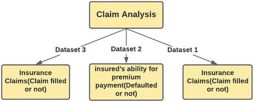
In this study, we used three separate datasets to do claim analysis. As Figure 1 shows, all three datasets have a categorical target variable. As a result, the analyses are carried out using classification algorithms.

Figure 1. The target variable in the three datasets.

Data Collection

Data collection is the first step in the ML process. Data can be gathered using a variety of sources and methods. The datasets for this study were obtained from Kaggle.com. Table 2 shows the description of the three datasets that we used in our study.

Table 2. Overview of the three insurance dataset

Dateset_1	Dataset_2	Dataset_3
The dataset used in this case study was sourced from Kaggle.com. There are 10302 rows and 25 features in total. The details of all the columns in the dataset: INDEX: ID Variable (not use) AGE: Age of the driver. BLUEBOOK: Value of vehicle. CAR_AGE: Vehicle age. CAR_TYPE: Type of car. CAR_USE: Vehicle use. Commercial CLM_FREQ: claims frequency (past 5 years EDUCATION: Max education level. HOMEKIDS: children at home. HOME_VAL: Home value. INCOME: Income. JOB: Job category. KIDSDRIV: driving children. MSTATUS: Marital status. MVR_PTS: Motor vehicle record points. OLDCLAIM: Total claim value (past 5 years). PRENT1: Single parent. RED_CAR. REVOKED: License revoked (past 7 years). SEX: Gender. TIF: Time in force. TRAVTIME: Distance to work. residence: Urban vs. rural YOJ: Years on job. Claim filled (Target variable): insured filled a claim, or not	The dataset used in this case study was sourced from Kaggle.com. 79,853 rows and 17 columns make up the dataset’s total. the details of all the columns in the dataset: id: Unique customer ID percent of the premium paid by cash credit age in days: age of the customer in days Income: Income of the customer Marital Status: Married/Unmarried Number of vehicles owned by the insured Count_3-6_months_late: Number of times premium was paid 3–6 months late Count_6-12_months_late: Number of times premium was paid 6–12 months late Count_more_than_12_months_late: Number of times premium was paid more than 12 months late Risk score: Risk score of customers (similar to credit score) Number of dependents in the family of the customer Accommodation: Owned /Rented number of premiums paid: Number of premiums paid till date sourcing channel: Channel through which customer was sourced residence area type: Residence type of the customer premium: Total premium amount paid till now default: 0 indicates that customer has defaulted the premium and 1 indicates that customer has not defaulted	The dataset used in this case study was sourced from Kaggle.com. 1,488,028 rows and 59 columns make up the dataset’s total. We examine data provided by Porto Seguro, a major Brazilian automaker. The database is maintained safe and confidential, and the personal information of the clients is encrypted. Before modifying the dataset to build the ML model, it is vital to understand how it was structured. A data description has also been released, which includes important information on the data preparation as following: A value of “-1” denotes that a value was missing. Binary features are labeled “bin” while categorical features are labeled “cat.” There are two types of features: continuous and ordinal. “ind”, “reg”, “car”, and “calc” all refer to features that belong in the same general category. A customer’s personal data, such as their name, is referred to as “ind.” A customer’s area or location information is referred to as “reg.” “car” is related to car itself Porto Seguro’s calculated features are referred to as “calc.” Target variable 1- insured filled a claim,0 otherwise

Data Preparation

In Data Preparation, data is transformed so that an ML algorithm can use it. And it has the potential to have an impact on the model’s performance. Data cleaning, exploratory data analysis (EDA), normalization, encoding, solving the imbalanced data problem, and dimensionality reduction are all part of the process of data preparation.

Data Cleaning

Depending on the dataset, the features that include missing values are either eliminated the whole feature or alter these missing values. In this study, we removed two variables from the third data set because they had the most missing values in the third dataset. Where In the third dataset, we find that around 2.4% of the data are missing values. And the two features we removed have a high percentage of missing values. Following the removal of these two variables, the dataset’s missing values drop to only 0.18%. For the other features in the three datasets, the mode of the column values is used to replace missing values in category and binary variables. In contrast, the mean of the column values is used to fill in missing values in all continuous variables.

Exploratory Data Analysis

Exploratory data analysis is a tool for better understanding data before using an ML algorithm. It is accomplished by visualizing data using various graphs in order to comprehend the various aspects of the data.

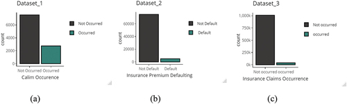
Figure 2 shows the distribution of the target variables in the three datasets. In dataset_1(a) the ratio between the non-occurred and occurred claims is 73% to23%, for the dataset_2(b), the ratio between the not defaulted to default is 94% to6%, and for the dataset_3(c), the ratio between the non-occurred and occurred claims is 96.4% to3.6%. This refers to the datasets suffer from imbalanced data problem especial in the second and third datasets.

Figure 2. The distribution of the binary target variable for the datasets.

Transformation

As most ML algorithms cannot process categorical data, all categorical data is consolidated into an understandable numerical format.

normalization

In the case of categorical data, feature engineering is done using feature encoding techniques. Due to the large number of algorithms used in ML, they only work with factors and continuous features because they’re built on mathematical models and techniques. Besides the encoding, we applied a Normalization for the data. Normalization is a technique for uniformly scaling all of the values in a dataset between 0 and 1. The normalizing formula is as follows:

(1) $X_{norm}=\frac{X-X_{min}}{X_{max}-X_{min}}$(1)

ML Classifiers

K-nearest Neighbor (KNN)

The K-nearest neighbor (KNN) algorithm is a basic algorithm that predicts each observation based on how similar it is to other observations. KNN is a memory-based algorithm. This means that the training samples are needed at run-time, and predictions are formed based on sample associations. As a result, KNNs are sometimes known as lazy learners (Cunningham and Jane Delany 2021).

The Strengths of the KNN Algorithm are as Follows:

• The algorithm is very simple to understand.

• There is no computational cost during the learning process; all the computation is done during prediction.

• It makes no assumptions about the data, such as how it’s distributed.

The Weaknesses of the KNN Algorithm are These:

• It cannot natively handle categorical variables (they must be recoded first, or a different distance metric must be used).

• When the training set is large, it can be computationally expensive to compute the distance between new data and all the cases in the training set.

• The model can’t be interpreted in terms of real-world relationships in the data.

• Prediction accuracy can be strongly impacted by noisy data and outliers.

• In high-dimensional datasets, KNN tends to perform poorly. This is due to a phenomenon called the curse of dimensionality.

Random Forest (RF)

RF is a commonly used machine-learning model that is based on Breiman et al decision’s theory (Breiman et al. 1984). The classification and regression tree (CART) algorithm is used to create trees in this model. If the response variable is a factor, RF will classify it; if the response is continuous, RF will do regression. In the RF model, CART grows a huge tree before pruning it. And according to (Grömping 2009), trimming a huge tree rather than growing a limited number of trees increases RF’s prediction accuracy.

The Strengths of the Random Forest are as Follows:

• It can handle categorical and continuous predictor variables

• It makes no assumptions about the distribution of the predictor variables.

• It can handle missing values in sensible ways.

• It can handle continuous variables on different scales.

• Ensemble techniques can drastically improve model performance over individual trees.

The Weaknesses of Tree-based Algorithms are These:

• The main disadvantage can be the loss of interpretability for the trained classifier model.

• High computational complexity.

Decision Tree (CART)

The decision tree is a graph or model that looks like a tree. Because it has its root at the top and grows downwards, it resembles an inverted tree. In comparison to other ways, this representation of the data has the advantage of being meaningful and simple to read. Each of the input attributes correlates to one of the tree’s internal nodes. The number of edges on a notional interior node is the same as the number of possible input attribute values. Given the values of the input attributes represented by the path from the root to the leaf, each leaf node represents a value of the label attribute. In the Simple Cart algorithm, decision trees are built by separating each decision node into two separate branches based on various separation criteria (Noori 2021).

The Strengths of Tree-based Algorithms are as Follows:

• Tree-building has a basic intuition, and each tree is easily interpretable.

• Categorical and continuous predictor variables are supported.

• There are no assumptions made regarding the predictor variables’ distribution.

• It has a logical manner of dealing with missing values.

• It is capable of dealing with continuous variables on various scales.

The Weakness of Tree-based Algorithms is This:

• Individual trees are prone to overfitting.

Logistic Regression (LR)

The (linear) relationship between a continuous response variable and a set of predictor variables is approximated using linear regression. However, linear regression is not acceptable when the response variable is binary (i.e., Yes/No). Fortunately, analysts can use an approach that is comparable to linear regression in many ways called the logistic regression Faraway (2016).

The Strengths of the Logistic Regression Algorithm are as Follows:

• It can handle both continuous and categorical predictors.

• The model parameters are very interpretable.

• Predictor variables are not assumed to be normally distributed.

The Weaknesses of the Logistic Regression Algorithm are These:

• It won’t work when there is complete separation between classes.

• It assumes that the classes are linearly separable. In other words, it assumes that a flat surface in n-dimensional space (where n is the number of predictors) can be used to separate the classes. If a curved surface is required to separate the classes, logistic regression will underperform compared to some other algorithms.

• It assumes a linear relationship between each predictor and the log odds. If, for example, cases with low and high values of a predictor belong to one class, but cases with medium values of the predictor belong to another class, this linearity will break down.

Feature Selection Methods

The feature selection procedure focuses on detecting and discarding redundant features from a dataset (Ziemba et al. 2014). The multidimensionality of the object to be allocated to a given class is one of the most basic concerns in classification tasks. The “dimensional curse” is a severe impediment that reduces the accuracy of classification systems. Reducing the dimensionality of feature space lowers computational and data collection costs, which improves predictions. This also aids in the reduction of execution time. We’ve applied three algorithms:

1. Relief (RE)

2. Symmetrical Uncertainty (SU)

3. Correlation-based Feature Selection (CFS).

Relief Feature Selection Technique

Relief assigns a weight to all the features in the dataset. Once these weights are established, they can be gradually changed (Pronab et al. 2021). The goal is to have a high weight for the most critical qualities and a low weight for the less important ones. To determine feature weights, Relief employs methods similar to those found in KNN.

Symmetrical Uncertainty (SU)

SU has been shown to be a good measure for choosing significant traits in a variety of research (Piao and Keun Ho). The SU is a correlation metric for a feature. The following is how to determine the Symmetrical Uncertainty between a feature and a class:

(2) $\mathrm{I}\mathrm{G}(\mathrm{F}|\mathrm{C})=\mathrm{H}\left(\mathrm{F}\right)-\mathrm{H}(\mathrm{F}|\mathrm{C})$(2)

(3) $\mathrm{S}\mathrm{U}\left(\mathrm{F},\mathrm{C}\right)=2\ast \mathrm{I}\mathrm{G}(\mathrm{F}|\mathrm{C})/\left(\mathrm{H}\left(\mathrm{F}\right)+\mathrm{H}\left(\mathrm{C}\right)\right)$(3)

Where IG(F|C) refer to the information gain of a feature F after watching class C. And the entropy of feature F and class C, respectively, is H(F) and H(C). Adjusts for an information gain deviation toward multi-valued attributes and normalizes the final score to the range [0, 1]. ‘1ʹ indicates that we are completely informed based on the at-tribute, allowing us to forecast the object’s class; ‘0ʹ indicates that no information is available after examining the attribute, therefore no prediction is feasible.

Correlation-based Feature Selection (CFS)

CFS evaluates the value of features using a correlation-based heuristic. A well-known feature selector wrapper utilizes a special learning method to direct its search for good features to evaluate CFS’s effectiveness. At first, a matrix of mutual attribute correlation and attribute-class correlation is computed. And the “Best First” method is used for forwarding search (Hall and Smith 1999). An important part of the CFS algorithm is an evaluation heuristic for a subset’s value or merit. Individual features’ usefulness in predicting class labels and intercorrelation between them are both taken into account by this heuristic. The heuristic’s hypothesis can be stated as follows: good feature sub-sets contain traits that are highly correlated (predictive of) the class but uncorrelated (not predictive of) each other.

The heuristic is formalized in the following equation:

(4) $Meri{t}_s=\frac{k\overline{r_{cf}}}{\sqrt{k+k\left(k-1\right)\overline{r_{ff}}}}$(4)

where $Meri{t}_s$ is a feature subset’s heuristic “merit” $S$ including $k$ attributes, $\overline{r_{cf}}$ is the average correlation between feature classes ($f\in S$), and $\overline{r_{ff}}$ is the average intercorrelation of features. In actuality, Equation 4(4) $Meri{t}_s=\frac{k\overline{r_{cf}}}{\sqrt{k+k\left(k-1\right)\overline{r_{ff}}}}$(4) is the Pearson’s correlation, with all variables normalized. The numerator indicates how predictive a set of traits is of the class, while the denominator indicates how much duplication exists among them. Irrelevant traits are ignored by the heuristic because they are given poor predict with the target class.

Resampling Methods

When the number of classes in the training set is uneven, i.e., the target class distribution is significantly unbalanced, ML classifiers develop models that prefer to categorize all objects as belonging to the majority class in order to maximize the overall accuracy of the model. But this leads to low accuracy for the minority class, whose objects are underrepresented in the training set, despite the fact that this minority class is often critical (Pozzolo et al. 2015). The techniques of random under-sampling and random oversampling are two of the most prevalent in ML and are also relatively basic. And Table 3 shows the basis characteristics of each resampling method.

Table 3. Characteristics of the resampling methods

Method	Essence of the Method	Advantages and Disadvantages
Random Over Sampling method	Random oversampling entails replicating minority class examples at random and adding them to the training dataset. By repeating the original samples, this approach increases the size of the dataset. The point is that the random over sampler does not generate new samples and does not change the diversity of samples (Hui et al. 2013).	Advantages: Replacement is used to select examples from the training dataset at random. A new “more balanced” training dataset will have examples from the minority class that can be picked and added to more than once. Where the examples from the original training dataset will be returned or “replaced” with examples from the new training dataset, allowing them to be selected again. Disadvantages: puts at risk of overfitting the classifier model by shifting the model toward the minority class; not adding any new valuable objects of the minority class; classifier training is significantly extended by increasing the size of the training set
Random Under-Sampling method	Random under-sampling is the process of removing samples from the majority class from the training dataset at random. One of the easiest ways for dealing with the unbalanced data problem is the under-sampling method (Ghorbani and Ghousi 2020). And to balance the majority and minority classes, this strategy under-samples the majority class.	Advantages: When the amount of data collected is sufficient, under-sampling may be a useful method to apply. Disadvantages: The random under-sampling has the drawback of removing cases from the majority class that could be informative, essential, or even critical in fitting a robust decision boundary. There is no method to recognize or preserve “good” or more information-rich instances from the majority class because examples are removed at random.

Discretization Methods

By using feature discretization, some classification algorithms increase their performance. Continuous characteristics are separated into ranges or intervals, resulting in numerical data being converted to nominal data. Because continuous data can be discretized in an endless number of ways, the fundamental challenge with feature discretization is suitable to cut point selection. The ideal discretization method would locate a small number of cut points and divide data into appropriate bins. There are two types of discretization techniques: supervised and unsupervised. Because the supervised methods use class distribution to which each object belongs as extra information, the supervised’s results are superior to the second group. A large number of approaches use class entropy, which is a measure of uncertainty in a finite range of classes. And to accomplish discretization, the entropy of different splits is calculated and compared to the entropy of the dataset without divides, and until the search stop requirement is met, it runs recursively (De Sá et al. 2013). The Minimal Description Length Principle (MDLP) heuristic approach, for example, can be employed here. If the provided criterion is not met, this approach determines whether or not to accept the current cutoff point candidate, ending the recursion. One of the finest supervised discretization approaches is entropy-based discretization using the MDLP stop criterion. By comparing entropy values, it calculates the information gain score of a feasible cut point. The entropy of the input period is compared to the weighted sum of entropies for two output intervals for each cut point investigated. There are various distinct criteria for MDLP halting conditions. And in our study, we will use The Fayyad criterion (Fayyad and Irani 1993).

Evalution Methods

Comparing and determining the optimal model requires evaluating the performance of classifiers. ML algorithms can be measured and checked in a variety of ways. This work employs a variety of evaluation techniques, including prediction accuracy, sensitivity, specificity, and AUC. And for more trustworthy and powerful assessing and comparing, we will also use a statistical assessment technique.

Confusion Matrix

The terms TP, TN, FN, and FP are used to describe Sensitivity (SE), Specificity (SP), and classification Accuracy (AC).

(5) $Sensitivity=\frac{TP}{TP+FN}$(5)

(6) $Specificity=\frac{TN}{TN+FP}$(6)

(7) $Accuracy=\frac{TN+TP}{TN+TP+FN+FP}$(7)

The Sensitivity of a model (also known as the true positive rate) is a metric that evaluates the accuracy of correctly identified positive examples (actual events). While the specificity of a model (also known as the true negative rate) is a metric that quantifies the proportion of correctly identified negative examples (non-actual events). The useful classifier must give highly accurate results for the Sensitivity and the specificity simultaneously.

The accuracy represents the ratio of correct predictions to total samples. While accuracy is simple to realize, it overlooks several important criteria that must be addressed when evaluating a classifier’s performance. When a set of samples of the target class is unbalanced in the data set, the accuracy will be useless because the algorithm forecasts the value of the majority classes for all predictions. In such instances, the AUC is a useful option because it considers the class distribution and is thus less likely to suffer from the data set’s imbalance.

where:

• TP refers to the true positives, representing the number of instances the algorithm has predicted the positive class accurately.

• FN refers to the false negatives, representing the number of instances the algorithm incorrectly forecasts the negative class.

• FP refers to the false positives, representing the number of instances the algorithm incorrectly forecasts the positive class.

• TN refers to the true negatives, representing the number of instances the algorithm properly forecasts the negative class.

In ML, evaluating models in the face of rare cases is critical. Despite the fact that Accuracy is the most often used classification assessment metric, it may not be an acceptable solution for unbalanced data sets due to bias toward the majority class. In such instances, the AUC is a useful option because it considers the class distribution and is thus less likely to suffer from the data set’s imbalance (Haixiang et al. 2017).

Area Under Receiver Operating Characteristic Curve (AUROC)

The (AUROC) can be used to evaluate the classification’s quality. ROC is a graphic representation of a predictive model’s performance created by sketching the quantitative properties of binary classifiers obtained from such a model using a range of cutoff points. And this shows how the True Positive Rate (TPR) and False Positive Rate (FPR) are related. TPR and FPR can be calculated by the following equations:

(8) $TPR=\frac{TP}{TP+FN}$(8)

(9) $FPR=\frac{FP}{FP+TN}$(9)

The accuracy of the classifier is measured by AUROC. It’s estimated as probability thresholds for the next event – whether the object in question is negative or positive. AUC is the area below the ROC in terms of geometry. The higher the AUROC value, the better the model’s classification outcomes. AUROC less than 0.5 indicates an invalid classifier, i.e., one that is poorer than random, AUROC = 0.5 indicates a random classifier, and AUROC = 1 indicates an ideal classifier (Chawla et al. 2002).

Statistical Analysis

Evaluating and comparing the performance of the classifiers is a crucial step. Even though evaluation methods such as sensitivity, specificity, and classification accuracy are simple to implement, the findings they produce can be deceptive. Determining the best model or approach is, therefore, a complex issue. Statistical significance tests will be used to tackle this issue based on the AUC values. A one-way analysis of variance (ANOVA) is a typical statistical test for comparing two or more related sample means. In the ANOVA test, the null hypothesis is that all models perform similarly and that the reported differences are unimportant (Fisher 1956). And we also will use the Friedman test (Friedman 1937), which is a non-parametric variant of the ANOVA test, which can be used to investigate differences among the methods. The Friedman test’s null hypothesis is that all methods perform equally; however, rejecting this null hypothesis means that one or more approaches perform differently. The Freidman test ranks each method’s data before analyzing the rank values (Friedman 1940). As a result, the Friedman test produces a sum of ranks for each approach, which will help us to figure out which method is the most efficient among the others.

Research Procedures

For each dataset, the dataset will divide into two sections: training and testing. 70% of the data is assigned to the training phase, while the remaining 30% is assigned to the testing phase based. In our research topic, there are various combinations will be investigated of filter methods (SU, CFS, Relief), classifier models (LR, DT, KNN, RF), resampling methods (without resampling, random under-sampling, random oversampling) and feature discretization (without discretization, Fayyad criterion).

With the number of methodological approaches studied, each dataset has 60 possible scenarios for each dataset. The research study was divided into four general scenarios, each using the following approach combinations:

1. Apply the classification algorithms without any resampling or feature selection methods, or feature discretization.

2. Apply the classification approaches based on only resampling methods.

3. Apply the feature selection, followed by resampling methods, then the classification algorithms.

4. Apply the feature discretization followed by features selection methods, followed by resampling methods, then the classification algorithms.

All research scenarios enabled to define:

• Examine the effect of data resampling on the performance of ML classifiers.

• Examine the impact of features selection methods followed by data resampling approaches on ML classifiers performance.

• Examine the impact of the feature discretization method followed by features selection methods, followed by resampling methods on ML classifiers performance.

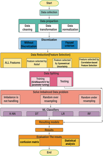
The research study that was conducted is shown in Figure 3. We should note that the features selection was made to the training set, and the results were employed in the testing set. This was an important step in ensuring that the training and testing sets were completely consistent. For example, relevant features were chosen from the training set and superfluous features were also purged from the testing set. Data resampling was the only processing method employed only for training and not for testing cases.

Figure 3. Working diagram of proposed model.

Hyperparameter Tuning

To prevent overfitting and underfitting, we must tune model parameters within stable zones where training and validation scores do not change dramatically. The grid search technique, which is a prominent tuning tool in the insurance area, has been used to optimize the model’s parameters. Where In order to achieve the highest ROC values, GridSearchCV was utilized. Table 4 displays the parameter search ranges and optimum values for the models.

Table 4. The optimal values for several model parameters used in this study

ML	Range	Optimal parameters for Dataset_1	Optimal parameters for Dataset_2	Optimal parameters for Dataset_3
KNN	K [1:50]	K = 21	K = 5	K = 9
DT	cp [0:1]	cp = .0058	cp = .0020	cp = .0002
RF	mtry [1:100]	mtry = 37	mtry = 19	mtry = 40
LR	No tunning parameters

Table 4 shows the hyper-parameter tuning on the models used in this paper. Where K is the Number of Neighbors, C is the Confidence Threshold, M is the Minimum Instances Per Leaf, cp is the Complexity Parameter and Mtry is the number of Randomly Selected Predictors

Results and Discussion

Table 5 shows the results of the accuracy, sensitivity, specificity, and AUC values for all ML methods. Accuracy is one of the most widely used methods for assessing an algorithm’s performance. While accuracy is simple to realize, it overlooks several important criteria that must be addressed when evaluating a classifier’s performance. When a set of samples of the target class is unbalanced in the data set, the accuracy will be useless because the algorithm forecasts the value of the majority classes for all predictions. In such instances, the AUC is a useful option because it considers the class distribution and is thus less likely to suffer from the data set’s imbalance.

Table 5. The performance of the ML models on the different datasets

	Data_1				Data_2				Data_3
KNN	0.7745	0.9515	0.2435	0.598	0.9389	0.9951	0.0985	0.547	0.9619	1	0	0.5
RO+KNN	0.6632	0.6819	0.6569	0.666	0.8142	0.8386	0.4486	0.644	0.8157	0.8416	0.1657	0.504
RU+KNN	0.7129	0.7259	0.6741	0.7	0.8166	0.833	0.5717	0.702	0.6249	0.6311	0.468	0.55
RE+RO+KNN	0.6632	0.6635	0.6623	0.659	0.8124	0.834	0.4924	0.663	0.8103	0.8352	0.1831	0.509
SU+RO+KNN	0.6527	0.6421	0.6846	0.666	0.8095	0.8315	0.4846	0.658	0.8196	0.8439	0.2093	0.527
CFS+RO+KNN	0.636	0.6316	0.6492	0.64	0.8125	0.825	0.624	0.725	0.8162	0.8415	0.18023	0.511
RE+RU+KNN	0.7142	0.7198	0.6976	0.71	0.8158	0.828	0.6343	0.731	0.5681	0.57207	0.46802	0.52
SU+RU+KNN	0.7136	0.7298	0.6649	0.697	0.8237	0.8388	0.5988	0.719	0.5811	0.58261	0.5436	0.563
CFS+RU+KNN	0.6959	0.7001	0.6832	0.692	0.8125	0.825	0.6284	0.727	0.5683	0.57011	0.52326	0.547
FC+RE+RO+KNN	0.6982	0.6914	0.7186	0.705	0.7719	0.784	0.5929	0.688	0.6322	0.6383	0.47965	0.559
FC+SU+RO+KNN	0.7074	0.7036	0.7186	0.665	0.7722	0.7818	0.6297	0.706	0.588	0.591	0.529	0.56
FC+CFS+RO+KNN	0.7159	0.7512	0.6099	0.684	0.8147	0.8297	0.5921	0.688	0.6512	0.656827	0.50968	0.5833
FC+RE+RU+KNN	0.6579	0.6512	0.678	0.711	0.7822	0.786	0.7262	0.756	0.6134	0.6185	0.48547	0.552
FC+SU+RU+KNN	0.7237	0.725	0.7199	0.736	0.7971	0.8037	0.6993	0.752	0.5929	0.59604	0.51453	0.555
FC+CFS+RU+KNN	0.6609	0.636	0.7356	0.7	0.844	0.8619	0.5778	0.7157	0.7274	0.739	0.436	0.588
LR	0.7912	0.9079	0.4411	0.674	0.94	0.9945	0.1253	0.55	0.9617	1	0	0.5
RO+LR	0.7273	0.7193	0.7513	0.735	0.7898	0.7942	0.7238	0.759	0.6321	0.63575	0.5407	0.588
RU+LR	0.727	0.7211	0.7448	0.733	0.7872	0.7912	0.727	0.759	0.5948	0.59685	0.5436	0.57
RE+RO+LR	0.7234	0.7097	0.7644	0.713	0.7908	0.7949	0.7291	0.762	0.6322	0.6354	0.5523	0.594
SU+RO+LR	0.7267	0.718	0.7526	0.715	0.7906	0.7952	0.7216	0.758	0.6332	0.63691	0.5407	0.589
CFS+RO+LR	0.6966	0.6997	0.6872	0.693	0.7921	0.7985	0.697	0.748	0.7094	0.7212	0.41279	0.567
RE+RU+LR	0.7149	0.7067	0.7395	0.723	0.7175	0.7243	0.6156	0.67	0.5768	0.57798	0.54651	0.562
SU+RU+LR	0.7234	0.7176	0.7408	0.729	0.7869	0.7911	0.7238	0.757	0.5674	0.5683	0.5465	0.557
CFS+RU+LR	0.709	0.7163	0.6872	0.702	0.7888	0.7947	0.7013	0.748	0.7357	0.7498	0.38081	0.565
FC+RE+RO+LR	0.708	0.7032	0.7225	0.737	0.79	0.7939	0.7321	0.763	0.6091	0.61074	0.56686	0.589
FC+SU+RO+LR	0.7106	0.7058	0.7251	0.735	0.7927	0.7967	0.7341	0.765	0.6063	0.60692	0.59012	0.599
FC+CFS+RO+LR	0.6923	0.6866	0.7094	0.698	0.8173	0.8298	0.6323	0.731	0.5975	0.59639	0.625	0.616
FC+RE+RU+LR	0.709	0.7084	0.7107	0.71	0.7856	0.7891	0.7328	0.761	0.5582	0.55691	0.59012	0.574
FC+SU+RU+LR	0.7169	0.7128	0.7291	0.721	0.7951	0.7995	0.7301	0.765	0.6101	0.61179	0.56686	0.589
FC+CFS+RU+LR	0.6943	0.6918	0.7016	0.697	0.9367	1	0	0.5	0.6662	0.67188	0.52326	0.592
DT	0.7676	0.9376	0.2579	0.599	0.938	0.9941	0.09957	0.547	0.9619	1	0	0.5
RO+DT	0.6867	0.6853	0.6911	0.68	0.7549	0.7549	0.7505	0.753	0.4848	0.4777	0.6627	0.57
RU+DT	0.601	0.5238	0.8325	0.693	0.7537	0.7541	0.7473	0.751	0.5114	0.50758	0.60756	0.558
RE+RO+DT	0.6124	0.5439	0.8181	0.681	0.7086	0.7034	0.7853	0.747	0.6116	0.61538	0.51744	0.566
SU+RO+DT	0.6124	0.5439	0.8181	0.681	0.7086	0.7034	0.7853	0.744	0.4576	0.44807	0.69767	0.573
CFS+RO+DT	0.6435	0.6176	0.7212	0.669	0.8125	0.825	0.6284	0.727	0.4095	0.3972	0.718	0.558
RE+RU+DT	0.693	0.6918	0.6963	0.685	0.6393	0.6247	0.8549	0.74	0.7677	0.78442	0.34884	0.567
SU+RU+DT	0.7051	0.7254	0.644	0.685	0.6393	0.6247	0.8549	0.74	0.5817	0.58307	0.54651	0.563
CFS+RU+DT	0.6972	0.7014	0.6846	0.693	0.8125	0.825	0.6284	0.727	0.8551	0.8809	0.2093	0.545
FC+RE+RO+DT	0.638	0.5932	0.7723	0.683	0.7079	0.7027	0.7853	0.744	0.5474	0.54371	0.63953	0.598
FC+SU+RO+DT	0.6615	0.6312	0.7526	0.665	0.7079	0.7027	0.7853	0.744	0.4533	0.44263	0.72093	0.582
FC+CFS+RO+DT	0.6697	0.6897	0.6099	0.674	0.8143	0.8246	0.6613	0.736	0.6002	0.60125	0.57267	0.587
FC+RE+RU+DT	0.6576	0.6504	0.6793	0.692	0.5988	0.5808	0.8654	0.723	0.6216	0.62487	0.5407	0.58
FC+SU+RU+DT	0.7061	0.7189	0.6675	0.692	0.5936	0.5742	0.8798	0.727	0.5718	0.57323	0.53488	0.554
FC+CFS+RU+DT	0.6295	0.5897	0.7487	0.691	0.85574	0.87546	0.5625	0.7134	0.7876	0.80688	0.30233	0.555
RF	0.7905	0.9044	0.449	0.656	0.9388	0.9946	0.1049	0.56	0.9619	1	0	0.5
RO+RF	0.781	0.8787	0.4882	0.69	0.9371	0.9908	0.1349	0.563	0.9617	1	0	0.5
RU+RF	0.7214	0.7093	0.7579	0.722	0.7628	0.7625	0.7666	0.763	0.6437	0.64895	0.51163	0.58
RE+RO+RF	0.7849	0.8808	0.4974	0.686	0.9363	0.9883	0.1661	0.577	0.9617	1	0	0.5
SU+RO+RF	0.7823	0.88	0.4895	0.687	0.9333	0.9847	0.1733	0.579	0.9611	0.9993	0.0029	0.501
CFS+RO+RF	0.7103	0.8001	0.4411	0.621	0.8126	0.8256	0.6198	0.723	0.9551	0.99282	0.00872	0.501
RE+RU+RF	0.71	0.6975	0.7474	0.712	0.775	0.7771	0.7439	0.761	0.5901	0.59338	0.50872	0.551
SU+RU+RF	0.7103	0.6945	0.7579	0.716	0.7828	0.7859	0.7374	0.762	0.6358	0.64096	0.50581	0.573
CFS+RU+RF	0.6949	0.6966	0.6898	0.693	0.8125	0.825	0.6284	0.727	0.655	0.66146	0.49419	0.578
FC+RE+RO+RF	0.7453	0.8171	0.5301	0.674	0.8058	0.8278	0.4793	0.654	0.6734	0.6838	0.41279	0.548
FC+SU+RO+RF	0.7047	0.6975	0.7264	0.66	0.8166	0.8438	0.4143	0.629	0.668	0.67801	0.4157	0.547
FC+CFS+RO+RF	0.7489	0.8106	0.5641	0.693	0.8147	0.833	0.5442	0.693	0.6783	0.68635	0.47674	0.61
FC+RE+RU+RF	0.7424	0.8245	0.4961	0.739	0.7704	0.7714	0.7551	0.765	0.6681	0.67558	0.47965	0.578
FC+SU+RU+RF	0.7057	0.6958	0.7356	0.74	0.7822	0.7851	0.738	0.764	0.6652	0.67222	0.48837	0.58
FC+CFS+RU+RF	0.7129	0.7346	0.6479	0.697	0.866	0.886075	0.5671	0.7185	0.6887	0.69665	0.48837	0.63

The most important outcome from Table 5 is the low performance of all algorithms with the initial scenario. Where we should note that algorithms do not get a good AUC-score when using the original data; thus, algorithms do not work well across all classes. The findings show that machine learning algorithms do not produce reliable results and that most classifiers cannot predict all target classes using datasets before utilizing resampling and features selection methods. As a result, resolving the problem of unbalanced data and reducing dimensionality are critical. On the other hand, after applying feature discretization, resampling methods and feature selection methods, The AUC values of all ML models have improved noticeably. For example, in the first dataset, the RF obtained the result of 65.6% with the AUC test using the first scenario, whereas the outcome is improved to the 74% using the FC+SU+RU +RF method in the fourth scenario. And in the second dataset, the LR obtained the result of 56% with the AUC test using the first scenario, whereas the outcome is improved to the 76.5% using the FC+ SU +RU+LR model in the fourth scenario. Furthermore, in the third dataset, the RF achieved the result of 50% with the AUC test with the first scenario, whereas the outcome is improved to the 63% with the FC+ CFS+RU+RF method in the fourth scenario.

Table 5 shows the performance of the ML models on the different datasets. Where KNN is the K-nearest neighbour model, LR is the logistic regression model, DT is the decision tree model, RF is the random forest model, RO is the random over resampling method, RU is the random under resampling method, RE is the Relief method, SU is the symmetrical uncertainty method, and CFS is the correlation-based feature selection method, and FC is referred to the Fayyad criterion method.

Table 5 shows the importance of using feature discretization, resampling methods and feature selection methods to increase the accuracy of the ML model performance, where after utilizing feature discretization, various resampling approaches and feature selection methods, the outcomes indicates that algorithms do not overlook any classes. For example, in the third dataset, all ML models in the first scenario are disregard one of the classes. This model, on the other hand, examines all classes with the other three scenarios.

Table 6 presents the top four classification results for the three datasets based on the AUC scores.

Table 6. Depicts the four top classification results for each dataset

	Dataset_1		Dataset_2		Dataset_3
	Model	AUC	Model	AUC	Model	AUC
1	FC+SU+RU+RF (Fourth scenario)	0.74	FC+SU+RO+LR/ FC+SU+RU+LR/ FC+RE+RU+RF (Fourth scenario)	0.765	FC+CFS+RU+RF (Fourth scenario)	0.63
2	FC+RE+RU+RF (Third scenario)	0.739	FC+SU+RU+RF (Fourth scenario)	0.764	FC+CFS+RO+LR (Fourth scenario)	0.616
3	FC+ RE+RO+LR (Fourth scenario)	0.737	RU+RF (Second scenario) FC+RE+RO+LR (Fourth scenario)	0.763	FC+CFS+RO+RF (Fourth scenario)	0.61
4	FC+SU+RU+KNN (Fourth scenario)	0.736	RE+RO+LR/ SU+RU+RF (Third scenario)	0.762	FC+SU+RO+LR (Fourth scenario)	0.599

Assuming no resampling or feature selection or discretization are applied, the best classification results were achieved as Table 7 shows:

Table 7. Depicts the four top classification results for each dataset in first scenario

Dataset_1		Dataset_2		Dataset_3
Model	AUC	Model	AUC	Model	AUC
LR	0.674	RF	0.56	All models	0.5

Table 7 presents the top classification results for the three datasets based on the ROC-AUC scores for models with the original data.

From Tables 6, 7, we can note that the first scenario achieved the worst results for all datasets compared to the rest of the scenarios. Obviously, dimensionality reduction and solving the imbalanced problem and applying the discretization technique is necessary in the insurance industry due to the lack of ability to explain classification or the need to collect a great amount of information in order to classify new cases; this means that the dimensionality reduction and also solving the unbalanced data problem in the insurance business and the discretization techniques are obviously required in the insurance industry

Statistical Test Results

Different resampling approaches and feature selection methods produce different data; thus, classifiers perform differently with these different datasets. As a result, determining the optimum approach for achieving the best results is quite difficult. Statistical significance tests such as ANOVA and Friedman tests can help with the difficult task of deciding on the optimal approach. After applying the ANOVA and Friedman test, we found the p-value is less than 0.05 based on the AUC values for the different methods in each dataset as Table 8 shows. As a result, the null hypothesis is rejected, and we will accept the alternative hypothesis that refers to there is a difference in the performance between the various methods inside each dataset.

Table 8. The ANOVA and the Friedman tests results

	Dataset_1	Dataset_2	Dataset_3
ANOVA	0.000316 ***	0.000793 ***	0.000985 ***
Friedman test	0.001276	0.01229	0.009876

Table 8 shows the p-value for the ANOVA and Friedman test based of the AUC values for the different methods inside each dataset.

Additional Information from Friedman Test Results

Table 9 shows the results of the Friedman test for the ranks, sum of ranks beside the median of the different methods based on the AUC values for the three datasets. And from Table 9, we can conclude the following results:

• According to dataset_1, the best results are achieved by the FC+ SU+RU method in the fourth scenario.

• According to dataset_2, the best results are achieved by the FC+SU+RU method in the fourth scenario

• According to dataset_3, the best results are achieved by the FC+CFS+RO method in the fourth scenario.

• According to the three datasets, the first scenario achieves the worst results.

Table 9. Additional information from Friedman test results

	Dataset_1			Dataset_2			Dataset_3
	Scenario 1			Scenario 1			Scenario 1
	Median	Sum of ranks	Rank	Median	Sum of ranks	Rank	Median	Sum of ranks	Rank
DATA	0.6275	5	15	0.5485	4	15	0.5	5	15
	Scenario 2			Scenario 2			Scenario 2
RO	0.685	31	9	0.6985	28.5	11	0.537	22	13
RU	0.711	50	2	0.755	43.5	3	0.564	32	7
	Scenario 3			Scenario 3			Scenario 3
RE+RO	0.6835	21.5	13	0.705	32	9	0.5375	26	10
SU+RO	0.684	26	10	0.701	26	12	0.55	31.5	8
CFS+RO	0.6545	8	14	0.726	30.5	10	0.5345	19	14
RE+RU	0.711	43.5	4	0.7355	35.5	6.5	0.5565	25	11
SU+RU	0.7065	41.5	5	0.7485	37.5	5	0.563	31	9
CFS+RU	0.693	36	7	0.727	32.5	8	0.556	23.5	12
	Scenario 4			Scenario 4			Scenario 4
FC+RE+RO	0.694	39	6	0.716	35.5	6.5	0.574	43	4
FC+SU+RO	0.665	22.5	12	0.725	38.5	4	0.571	45	3
FC+CFS+RO	0.6885	23.5	11	0.712	23.5	13	0.5985	57	1
FC+RE+RU	0.7105	46.5	3	0.7585	44	2	0.576	38.5	5
FC+SU+RU	0.7285	51.5	1	0.758	47.5	1	0.5675	35.5	6
FC+CFS+RU	0.697	34.5	8	0.71455	20	14	0.59	46	2

The Contributions to Theory and Its Ramifications

It may be argued that incorporating technology like ML into the insurance industry be able to be quite beneficial. It can assist identify and understanding customers in a much more comprehensive way than the insurance industry’s narrow description of their requirements and investing patterns. Where claim analysis can help improve the insurance policies and calculate more sustainable premiums for clients by understanding the claiming patterns and demography of the insureds. The profit ratio of the insurance policies can also be changed by analyzing the insurance company’s acceptance tendencies. In our study, it has been discovered that utilizing feature discretization, feature selection approaches and resampling methods before categorizing data with classification algorithms is really effective. Since not all features are equally important, and also the unbalanced data leads to a bias in favor of the dominant group. By using feature selection strategies, we can pick the best subset of features for the best outcomes. And by using the resampling procedures, we can help overcome the problem of unbalanced data. Also, Feature selection approaches and resampling procedures help reduce data overfitting, improve the algorithm’s accuracy, and shorten computing time. We believe that our work will help insurance economists choose and execute the best predictive models and related methodologies for modeling insurance data to enhance the area of insurance economics.

Conclusion and the Future Work

Insurance Data mining is a powerful analytical tool for uncovering important and relevant knowledge from insurance data. But it can run into issues like imbalanced data and the Dimensions curse. This research aims to demonstrate the impact of resampling strategies for solving the unbalanced data problem and feature selection methods for reducing data Dimensions. It should be noted that three separate insurance databases are employed. In addition, a number of classifiers are used to help draw more accurate conclusions about the different approaches. The results demonstrate that ML classifiers can’t predict some of the classes in the first scenario: While after applying resampling methods, feature selection methods and feature discretization to various data sets, the findings reveal that the performance of most ML classifiers has greatly improved, and all classes are predicted, indicating that the classifiers’ performance is improved. And also, the results show that classifiers perform differently on different data for the three datasets generated by applying the feature discretization, feature selection approaches and resampling methods, making it difficult to choose the optimum strategy. Thus, besides using evaluation measures such as Accuracy, sensitivity, and the AUC measures, the Friedman test was performed in this paper to determine the optimal approach. The findings of this paper confirm the following:

Based on the Friedman test:

• For the first data set, the most accurate result is achieved by the FC+SU+RU method in the fourth scenario.

• For the second data set, the most accurate result is achieved by the FC+SU+RU method in the fourth scenario.

• For the third data set, the most accurate result is achieved by the FC+CFS+RO method in the fourth scenario.

Moreover, the results show also the RF model is the best classifier because it achieved the most accurate AUC results for each dataset:

• For the first data set, the RF achieves the best performance with an AUC of 74% with the FC+SU+RU method in the fourth scenario.

• For the second data set, FC+SU+RO+LR/ FC+SU+RU+LR/ FC+RE+RU+RF in the fourth scenario achieve the best performance with an AUC of 76.5%.

• For the third data set, the RF achieves the best performance with an AUC of 63%with the FC+CFS+RU method in the fourth scenario.

Of fact, the aforementioned heuristics do not cover all aspects of selecting an effective strategy to the risk scoring problem. Where choosing a classification model will essentially entail balancing the inherent characteristics of classifiers.

This research can be developed in the following directions:

• For a better comparison and improved performance, new ensemble and hybrid classifiers can be developed, and also other techniques can be applied, such as new feature discretization methods besides new and hybrid resampling methods and new feature selection methods.

• Expanding the empirical analysis incorporating XAI (Explainable artificial intelligence) methods. Apply a post-processing technique such as Shapley values or Shapley Lorenz Values as described, for example, in (Giudici and Raffinetti 2021; Bussmann et al. 2021) to make the models more explainable

Data Availability Statement

Dataset_1: https://raw.githubusercontent.com/heathergeiger/Data621_hw4/master/insurance-evaluation-data.csv

Dataset_2: https://www.kaggle.com/prakharrathi25/premium-default-prediction/data

Dataset_3: https://www.kaggle.com/headsortails/steering-wheel-of-fortune-porto-seguro-eda/data

Disclosure Statement

No potential conflict of interest was reported by the author(s).

Correction Statement

This article has been republished with minor changes. These changes do not impact the academic content of the article.

Additional information

Funding

This work was supported by: The characteristic & preponderant discipline of key construction universities in Zhejiang province (Zhejiang Gongshang University- Statistics), Collaborative Innovation Center of Statistical Data Engineering Technology & Application, The National Natural Science Foundation of China (11971433).

References

- Barry, L., and A. Charpentier. 2020. Personalization as a promise: Can big data change the practice of insurance? Big Data & Society 7 (1):2053951720935143. doi:10.1177/2053951720935143.
- Breiman, L., Friedman, J.H., Olshen, R.A., and Stone, C.J. (1984). Classification And Regression Trees (1st ed.). (pp. 368). Routledge. https://doi.org/10.1201/9781315139470
- Briys, E., and F. De Varenne. 2001. Insurance: From Underwriting to Derivatives. In: Jacque L.L., Vaaler P.M. (eds) Financial Innovations and the Welfare of Nations. Springer, Boston, MA, pp 301-314. https://doi.org/10.1007/978-1-4615-1623-1_15, .
- Bussmann, N., P. Giudici, D. Marinelli, and J. Papenbrock. 2021. Explainable machine learning in credit risk management. Computational Economics 57 (1):203–1631. doi:10.1007/s10614-020-10042-0.
- Chawla, N. V., K. W. Bowyer, L. O. Hall, and W. Philip Kegelmeyer. 2002. SMOTE: Synthetic minority over-sampling technique. Journal of Artificial Intelligence Research 16:321–57. doi:10.1613/jair.953.
- Cunningham, P., and S. J. Jane Delany. 2021. k-Nearest neighbour classifiers - A tutorial. ACM Computing Surveys (CSUR) 54 (6):1–25. doi:10.1145/3459665.
- Das, D., C. Chakraborty, and S. Banerjee. 2020. A framework development on big data analytics for terahertz healthcare. In Amit Banerjee, Basabi Chakraborty, Hiroshi Inokawa, Jitendra Nath Roy (eds)Terahertz biomedical and healthcare technologies, 127–43. Elsevier. https://www.sciencedirect.com/science/article/pii/B9780128185568000070
- Das, S., S. Datta, H. Abbas Zubaidi, and I. Ali Obaid. 2021. Applying interpretable machine learning to classify tree and utility pole related crash injury types. IATSS Research.
- De Sá, C. R., C. Soares, A. Knobbe, P. Azevedo, and A. M. Jorge (2013). Multi-interval Discretization of Continuous Attributes for Label Ranking. In: Fürnkranz J., Hüllermeier E., Higuchi T. (eds) Discovery Science. DS 2013. Lecture Notes in Computer Science, vol 8140. Springer, Berlin, Heidelberg. https://doi.org/10.1007/978-3-642-40897-7_11
- Dhieb, N., H. Ghazzai, H. Besbes, and Y. Massoud. 2020. A secure ai-driven architecture for automated insurance systems: Fraud detection and risk measurement. IEEE Access 8:58546–58. doi:10.1109/ACCESS.2020.2983300.
- Faraway, J. J. 2016. Extending the linear model with R. Generalized linear, mixed effects and nonparametric regression models (2nd ed.). New York: Chapman and Hall/CRC. https://doi.org/10.1201/9781315382722
- Fayyad, U., and K. Irani. 1993. Multi-interval discretization of continuous valued attributes for classification learning. Proceedings of the 13th international joint conference on artificial intelligence, San Francisco, CA, USA; pp. 1022–1027.
- Fisher, R. A. 1956. Statistical Methods and Scientific Inference, Edinburgh: Oliver & Boyd. https://scholar.google.com/scholar_lookup?hl=en&publication_year=1956&author=R.+A.+Fisher&title=Statistical+Methods+and+Scientific+Inference
- Friedman, M. 1937. The use of ranks to avoid the assumption of normality implicit in the analysis of variance. Journal of the American Statistical Association 32 (200):675–701. doi:10.1080/01621459.1937.10503522.
- Friedman, M. 1940. A comparison of alternative tests of significance for the problem of m rankings. The Annals of Mathematical Statistics 11 (1):86–92. doi:10.1214/aoms/1177731944.
- Fung, H.-G., G. C. Lai, G. A. Patterson, and R. C. Witt. 1998. Underwriting cycles in property and liability insurance: An empirical analysis of industry and by-line data. The Journal of Risk and Insurance 65 (4):539–61. doi:10.2307/253802.
- Ghorbani, R., and R. Ghousi. 2020. Comparing different resampling methods in predicting students’ performance using machine learning techniques. IEEE Access 8:67899–911. doi:10.1109/ACCESS.2020.2986809.
- Giudici, P., and E. Raffinetti. 2021. Shapley-Lorenz eXplainable artificial intelligence. Expert Systems with Applications 167:114104. doi:10.1016/j.eswa.2020.114104.
- Gramegna, A., and P. Giudici. 2020. Why to buy insurance? An Explainable Artificial Intelligence Approach’, Risks 8:137.
- Grize, Y., W. Fischer, and C. Lützelschwab. 2020. Machine learning applications in nonlife insurance. Applied Stochastic Models in Business and Industry 36 (4):523–37. doi:10.1002/asmb.2543.
- Grömping, U. 2009. Variable importance assessment in regression: Linear regression versus random forest. The American Statistician 63 (4):308–19. doi:10.1198/tast.2009.08199.
- Günther, C.-C., I. Fride Tvete, K. Aas, G. Inge Sandnes, and Ø. Borgan. 2014. Modelling and predicting customer churn from an insurance company. Scandinavian Actuarial Journal 2014 (1):58–71. doi:10.1080/03461238.2011.636502.
- Guo, F., and Y. Fang. 2013. Individual driver risk assessment using naturalistic driving data. Accident Analysis & Prevention 61:3–9. doi:10.1016/j.aap.2012.06.014.
- Haixiang, G., L. Yijing, J. Shang, G. Mingyun, H. Yuanyue, and G. Bing. 2017. Learning from class-imbalanced data: Review of methods and applications. Expert Systems with Applications 73:220–39.
- Hall, M. A., and L. A. Smith (1999). Feature selection for machine learning: Comparing a correlation-based filter approach to the wrapper. FLAIRS conference.
- Hanafy Kotb, M., and R. Ming. 2021.Comparing SMOTE family techniques in predicting insurance premium defaulting using machine learning models. International Journal of Advanced Computer Science and Applications (IJACSA) 12 (9):2021. doi:10.14569/IJACSA.2021.0120970.
- Hanafy, M. O. H. A. M. E. D., and R. U. I. X. I. N. G. Ming. 2021c. USING MACHINE LEARNING MODELS TO COMPARE VARIOUS RESAMPLING METHODS IN PREDICTING INSURANCE FRAUD. Journal of Theoretical and Applied Information Technology 99:2819-2833.
- Hanafy, M., and R. Ming. 2021b. Machine learning approaches for auto insurance big data. Risks 9 (2):42. doi:10.3390/risks9020042.
- Hanafy, M., and R. Ming. 2021a. Improving imbalanced data classification in auto insurance by the data level approaches. International Journal of Advanced Computer Science and Applications (IJACSA) 12 (6). doi:10.14569/IJACSA.2021.0120656.
- Hassan, A. K. I., and A. Abraham. 2016. Modeling Insurance Fraud Detection Using Imbalanced Data Classification. In: Pillay N., Engelbrecht A., Abraham A., du Plessis M., Snášel V., Muda A. (eds) Advances in Nature and Biologically Inspired Computing. Advances in Intelligent Systems and Computing, vol 419. Springer, Cham. Berlin/Heidelberg, Germany, pp. 117–127 https://doi.org/10.1007/978-3-319-27400-3_11
- Huang, Y., and S. Meng. 2019. Automobile insurance classification ratemaking based on telematics driving data. Decision Support Systems 127:113156. doi:10.1016/j.dss.2019.113156.
- Hui, L., L. Jia, P-C. Chang, and J. Sun. 2013. Parametric prediction on default risk of Chinese listed tourism companies by using random oversampling, isomap, and locally linear embeddings on imbalanced samples. International Journal of Hospitality Management 35:141–51. doi:10.1016/j.ijhm.2013.06.006.
- Kowshalya, G., and M. N. 2018. Predicting fraudulent claims in automobile insurance. Paper presented at the 2018 Second International Conference on Inventive Communication and Computational Technologies (ICICCT).
- Krasheninnikova, E., J. García, R. Maestre, and F. Fernández. 2019. Reinforcement learning for pricing strategy optimization in the insurance industry. Engineering Applications of Artificial Intelligence 80:8–19. doi:10.1016/j.engappai.2019.01.010.
- Matloob, I., S. Ahmad Khan, F. Hussain, W. Haider Butt, R. Rukaiya, and F. Khalique. 2021. Need-Based and optimized health insurance package using clustering algorithm. Applied Sciences 11 (18):8478. doi:10.3390/app11188478.
- Noori, B. 2021. Classification of customer reviews using machine learning algorithms. Applied Artificial Intelligence 35 (8):567–88. doi:10.1080/08839514.2021.1922843.
- Paefgen, J., T. Staake, and F. Thiesse. 2013. Evaluation and aggregation of pay-as-you-drive insurance rate factors: A classification analysis approach. Decision Support Systems 56:192–201. doi:10.1016/j.dss.2013.06.001.
- Pesantez-Narvaez, J., M. Guillen, and M. Alcañiz. 2019. Predicting motor insurance claims using telematics data—XGBoost versus logistic regression. Risks 7 (2):70. doi:10.3390/risks7020070.
- Piao, Y., and R. Keun Ho. A Hybrid Feature Selection Method Based on Symmetrical Uncertainty and Support Vector Machine for High-Dimensional Data Classification. In: Nguyen N., Tojo S., Nguyen L., Trawiński B. (eds) Intelligent Information and Database Systems. ACIIDS 2017. Lecture Notes in Computer Science, vol 10191. Springer, Cham. Berlin/Heidelberg, Germany, pp. 721–727. https://doi.org/10.1007/978-3-319-54472-4_67
- Pozzolo, D., O. C. Andrea, R. A. Johnson, and B. Gianluca. 2015. Calibrating Probability with Undersampling for Unbalanced Classification, In 2015 IEEE Symposium Series on Computational Intelligence, pp. 159–166.
- Pronab, G., S. Azam, M. Jonkman, F. M. J. M. S. Asif Karim, E. Ignatious, S. Shultana, A. Reddy Beeravolu, F. De Boer, and F. De Boer. 2021. Efficient prediction of cardiovascular disease using machine learning algorithms with relief and LASSO feature selection techniques. IEEE Access 9:19304–26. doi:10.1109/ACCESS.2021.3053759.
- Rawat, S., A. Rawat, D. Kumar, and A. Sai Sabitha. 2021. Application of machine learning and data visualization techniques for decision support in the insurance sector. International Journal of Information Management Data Insights 1 (2):100012. doi:10.1016/j.jjimei.2021.100012.
- Richter, A. N., and T. M. Khoshgoftaar. 2018. A review of statistical and machine learning methods for modeling cancer risk using structured clinical data. Artificial Intelligence in Medicine 90:1–14. doi:10.1016/j.artmed.2018.06.002.
- Ringshausen, F. C., R. Ewen, J. Multmeier, B. Monga, M. Obradovic, R. van der Laan, and R. Diel. 2021. Predictive modeling of nontuberculous mycobacterial pulmonary disease epidemiology using German health claims data. International Journal of Infectious Diseases 104:398–406. doi:10.1016/j.ijid.2021.01.003.
- Sabbeh, S. F. 2018. Machine-learning techniques for customer retention: A comparative study. International Journal of Advanced Computer Science and Applications 9(2), 273-281. http://dx.doi.org/10.14569/IJACSA.2018.090238
- Saggi, M. K., and S. Jain. 2018. A survey towards an integration of big data analytics to big insights for value-creation. Information Processing & Management 54 (5):758–90. doi:10.1016/j.ipm.2018.01.010.
- Singh, R., M. P. Ayyar, T. Venkata Sri Pavan, S. Gosain, and S. Rajiv Ratn. Year. Automating Car Insurance Claims Using Deep Learning Techniques, 2019 IEEE Fifth International Conference on Multimedia Big Data (BigMM), 2019, pp. 199-207. doi: 10.1109/BigMM.2019.00-25
- Stucki, O. 2019. Predicting the Customer Churn with Machine Learning Methods: Case: Private Insurance Customer Data. Master’s Thesis. LUT University. 2019.
- Sundarkumar, G. G., and V. Ravi. 2015. A novel hybrid undersampling method for mining unbalanced datasets in banking and insurance. Engineering Applications of Artificial Intelligence 37:368–77. doi:10.1016/j.engappai.2014.09.019.
- Weerasinghe, K. P. M. L. P., and M. C. Wijegunasekara. 2016. A comparative study of data mining algorithms in the prediction of auto insurance claims. European International Journal of Science and Technology 5:47–54.
- Ziemba, P., M. Piwowarski, J. Jankowski, and J. Wątróbski (2014). Method of Criteria Selection and Weights Calculation in the Process of Web Projects Evaluation. In: Hwang D., Jung J.J., Nguyen NT. (eds) Computational Collective Intelligence. Technologies and Applications. ICCCI 2014. Lecture Notes in Computer Science, vol 8733. Springer, Cham, Switzerland; pp. 684–693. https://doi.org/10.1007/978-3-319-11289-3_69