Causal Structure Learning Algorithm Based on Partial Rank Correlation under Additive Noise Model

ABSTRACT

Aiming at the structural learning problem of the additive noise model in causal discovery and the challenge of massive data processing in the era of artificial intelligence, this paper combines partial rank correlation coefficients and proposes two new Bayesian network causal structure learning algorithms: PRCB algorithm based on threshold selection and PRCS algorithm based on hypothesis testing. We mainly made three contributions. First, we proved that the partial rank correlation coefficient can be used as the standard of independence test, and explored the distribution of corresponding statistics. Second, the partial rank correlation coefficient is associated with the correlation, and a causal discovery algorithm PRCB based on partial rank correlation and an improved PRCS algorithm based on hypothesis testing are proposed. Finally, comparing with the existing technology on seven classic Bayesian networks, it proves the superiority of the algorithm in low-dimensional networks; the processing of millions of data on three high-dimensional Bayesian networks verifies the high-efficiency performance of the algorithm in high-dimensional large sample data; the application performance of the algorithm is tested by performing fault prediction on the real power plant equipment measurement point data set. Theoretical analysis and experimental results have proved the superiority of the algorithm.

Introduction

In recent years, the problem of causality discovery has been a research hotspot in the field of artificial intelligence and knowledge discovery(Chen et al. 2021; Foraita et al. 2020; Zeng et al. 2021). Researchers have proposed a variety of models for representing causality, which are widely used in statistics, biomedicine, and data mining (Mazlack 2009). With the rise of artificial intelligence and the advent of the era of big data, all fields urgently need to deal with the challenges brought by massive data. As an important tool for analyzing data, the causal relationship model has become more and more important for its corresponding research problems. For example, emotion analysis has always been a hot topic in the field of artificial intelligence. Scholars have proposed a large number of machine learning and deep learning algorithms to carry out emotion recognition in text and other aspects (Aytuğ Onan, Korukoğlu, and Bulut 2016; Aytuğ Onan and Korukoğlu 2017; Aytug Onan and Toçoğlu 2021). However, with the increase of data volume and the continuous improvement of the performance requirements of emotion analysis, the prospects of algorithms that only focus on the classification results of emotion recognition are limited. Therefore, analyzing data from the perspective of causality, providing more abundant auxiliary information and effectively dealing with large amount of data can not only improve the competitiveness of algorithms, but also have certain practical significance.

Pearl of the University of California first proposed a Bayesian model based on probability theory and graph theory in 1988 (Pearl 2014). Typical Bayesian network structure learning algorithms can be roughly divided into three types: (1) Based on the method of dependency analysis, by learning the dependency and independent relationships between data variables, the conditional independent relationship structure between node variables is determined, which is thought as the structure of Bayesian networks. This type of algorithms are suitable for structure learning of sparse Bayesian networks, such as the classic SGS algorithm (Spirtes, Glymour, and Scheines 1989). (2) Based on the scoring search method, the core idea is to search in all structure spaces, by calculating a certain scoring function (measure the degree of fit between the network topology and the sample set), until the network structure that best matches the data set is found, such as K2 algorithm (Cooper and Herskovits 1992). Commonly used scoring methods mainly include Bayesian scoring, minimum description length scoring, Bayesian information criterion) and Akaike information criterion. Commonly used search algorithms mainly include greedy search method, branch and bound method, simulated annealing method and genetic algorithm. (3) Based on the hybrid method of dependency analysis and scoring search, the first two types of methods have their own advantages and disadvantages. The hybrid method combines the ideas of these two types of methods. First, rely on the analysis to obtain the node order or reduce the search space, and then perform the scoring search. To find the best network is the current research hotspot in this field, such as CB algorithm (Singh and Valtorta 1993), SC algorithm (Friedman, Nachman, and Pe’er 2013), MMHC algorithm (Tsamardinos, Brown, and Aliferis 2006), L1MB algorithm (Schmidt, Niculescu-Mizil, and Murphy 2007), PCB (Yang, Li, and Wang 2011) and PCS (Yang et al. 2016) algorithm.

In fact, most of the above algorithms have achieved relatively good results on discrete data or continuous data with multiple linear models. However, due to the assumption that the data distribution obeys a linear relationship, it cannot be applied to the causal structure learning on the multivariate nonlinear model, which limits the application prospects. In order to solve the Bayesian network structure learning problem of nonlinear data, Hoyer extended the Bayesian causality model and proposed an additive noise model that can describe nonlinear data. Subsequently, many corresponding independence test methods and their structure learning algorithms are generated. For example, Fukumizu proposed the HSIC independence test method (Fukumizu et al. 2007), which is based on the normalized cross-covariance operator of regenerative kernel Hilbert space, independent of the selection of kernel parameters, and has simple empirical estimation and good convergence. Tillman further proposed KPC algorithm based on the framework of PC algorithm and HSIC independence test method (Tillman, Gretton, and Spirtes 2009). Huang B made a series of improvements on Tillman’s work and proposed the CS-NOD algorithm (Zhang et al. 2017). In addition, there are LSMI independence test methods proposed by Yamada M (Yamada and Sugiyama 2010) and KCI independence test methods proposed by Zhang K (Zhang et al. 2012).

Data subject to a single linear distribution is not common in the real world, but there are a lot of nonlinear relations. For example, in the field of engineering and technology, the data transmitted by sensors that detect the status of plant equipment generally follows a nonlinear distribution. In the field of financial development, the fluctuation data of stock prices in the stock market can hardly meet the linear distribution. In the field of medical imaging, the image data obtained for the treatment of patients, even if the detection data set aided by image processing method is obtained, usually does not show linear distribution. Therefore, from the perspective of practical application, the study of the causal structure relationship under the nonlinear model has more practical significance and application value.

However, most current non-linear causality discovery algorithms have the following problems: (1) directly calculate the relationship between two variables and ignore the joint interference between the variables in the multivariable system, resulting in low accuracy. (2) Most nonlinear algorithms can also be used in linear models in theory, but many algorithms ignore the accuracy of linear models. Linear models can be regarded as a special form of nonlinear models. If the algorithm performs well on linear data and can handle complex nonlinear data, and it will be more competitive. (3) The algorithm has high time complexity. Many algorithms use theoretically powerful calculation methods in order to deal with complex nonlinear function relationships. However, obtaining results often takes a lot of time, which can only be applied to small sample data and cannot process large sample data in a limited time.

In response to the above problems, this paper starts from the study of partial Spearman correlation coefficient (Conover 1998) (a kind of partial rank correlation coefficient), and proposes two causal structure learning algorithms based on partial rank correlation – PRCB and PRCS. The algorithm we proposed can not only eliminate the joint interference between multiple variables, and thus detect the conditional correlation between system variables, but also has high accuracy in the learning of causal structure under linear and non-linear models. In addition, its efficient data processing capabilities can cope with the massive data problems generated by various industries in the era of big data, and it has broad application prospects. The partial rank correlation in this article is the partial Spearman correlation. Our contributions are mainly reflected in the following three aspects:

1. Under the additive noise model, it is proved that the partial rank correlation coefficient can be used as a measure of independence, and the correlation is redefined from the perspective of partial rank correlation.

2. Applying partial rank correlation coefficients to Bayesian structure learning, two new causal discovery algorithms are proposed: PRCB based on threshold selection and PRCS based on hypothesis testing, and the theoretical basis of the algorithm is explained.

3. The above algorithm has been carried out three parts of experiments: linear and nonlinear experiments with small sample data of low-dimensional networks, linear and nonlinear experiments with large sample data of high-dimensional networks, and application experiments on real data sets. A large number of experimental results show that the algorithm has excellent accuracy and time efficiency in linear and non-linear experiments, can effectively process a large amount of data generated in practical applications, and dig out hidden causal relationships.

The rest of this article is organized as follows. The second part reviews the previous research work and methods related to Bayesian structure learning. The third part introduces the partial rank correlation coefficient and proves that it can be used as a measure of independence. The fourth part proposes a causal structure learning algorithm based on partial rank correlation (PRCB algorithm and PRCS algorithm). The fifth part conducts experiments on the algorithm proposed in this paper and the comparison algorithm, and analyzes the results. The sixth part summarizes current work.

Related Work

The learning of Bayesian networks generally focuses on structure learning and parameter learning. Structural learning of Bayesian networks is the independent or dependent relationship among learning variables, which is represented by graphical (graph adjacency matrix), and is the main research field of Bayesian learning. Compared with the simple and standard parameter learning, structure learning needs to balance the accuracy and complexity of model building: on the one hand, it needs to build a network topology that can represent rich information to obtain reliable learning accuracy, and on the other hand, it needs to simplify the network model as much as possible to reduce the application maintenance cost and algorithm time complexity.

The current Bayesian network structure learning algorithms can be divided into two categories: one is the linear causality discovery algorithm that solves the problem of multivariate linear discrete or continuous data causal structure learning, and the other is a nonlinear causal discovery algorithm that deals with multivariate nonlinear discrete or continuous data causal structure learning problems. First introduce the linear causality discovery algorithm: Schmidt proposed the L1MB algorithm in 2007, and Jean-Philippe in 2008 proposed the TC algorithm (Pellet and Elisseeff 2008). Both algorithms can process continuous data generated by linear structural equation models that obey the linear multivariate Gaussian distribution. But the experiment shows that the accuracy of L1MB algorithm is not very high, and the TC algorithm has poor time performance and space performance. Wang proposed a two-phase (Two-Phase) algorithm (Wang and Chan 2010), which can process the data generated by the linear structural equation model and obey the linear multivariate Gaussian distribution or linear non-multivariate Gaussian distribution, but the algorithm’s time complexity is very high. Yang proposed a PCB algorithm based on partial correlation and an improved PCS algorithm. This algorithm can process the data generated by the linear structural equation model with arbitrary distribution of disturbances. It effectively combines local learning ideas and partial correlation techniques. Firstly, the skeleton of Bayesian network is reconstructed based on partial correlation, and then greedy hill-climbing search is performed to orient the edges to determine the final network graph, which has good structure learning ability and efficient time performance. The simulation results show that when the data set is generated by a linear structural equation model that is disturbed by arbitrary distribution, the algorithm has achieved excellent results in all indicators.

Next, introduce the development process of nonlinear causality discovery algorithm: Hoyer proposed additional noise model, linear Gaussian model and linear non-Gaussian model are special forms of this model, and proposed causal structure learning based on nonlinear regression and HSIC independence test method. Yamada et al. proposed a method based on least squares mutual information-independent regression (Yamada and Sugiyama 2010), and the experiment showed that this method was superior to HSIC regression in inferring causality. Mooij et al. proposed an evaluation method for causal structure based on MAP (Maximum A Posteriori) estimation (Mooij et al. 2009). This method effectively reduced the number of regression, but the computational complexity was still not negligible. In addition to research in the area of independent testing methods, there are other studies dealing with non-linear methods, such as: Gretton A et al. proposed the KMI (kernel mutual information) method (Gretton, Herbrich, and Smola 2003). Yamada M et al. proposed A cross-domain matching (CDM) framework based on square loss mutual information (SMI) (Yamada et al. 2015). Wu P et al. established an integration framework based on nonlinear independent component analysis (ICA) (Wu and Fukumizu 2020). Andrea’s model based on ESN reformulated the classical Granger causality (GC) framework for multivariate signals generated by any complex network, which can well detect nonlinear causality (Duggento, Guerrisi, and Toschi 2019). However, most of the algorithms have poor accuracy and high complexity, and can not be effectively applied to high-dimensional scenarios.

Based on the above problems, this paper starts from the PCB algorithm that achieves the best results in the linear model, and improves the PCB algorithm by combining the partial rank correlation coefficient, and proposes a causal discovery algorithm based on the partial rank correlation. This algorithm not only has the reasonableness of testing variables conditional correlation in the PCB algorithm and the efficient performance in terms of running time, it can also effectively deal with the causal relationship mining problem between the data generated by the nonlinear model, and it is more able to cope with the high-dimensional big data challenges in the era of artificial intelligence. We conducted a large number of comparative experiments with the above algorithm, and achieved excellent results in seven low-dimensional network small sample data and three high-dimensional network large sample data, and successfully applied to real data sets.

Summary of mathematical notations

Table

Notation	Mathematical meanings
G V X, Y, Z $X_i,Y_i$ $x_i$, $y_i$ PN(i) k$K_{\alpha }$	Directed acyclic graph Variable set in G A variable in V i-th N-dimensional feature vextor Value assignments for X and Y The candidate neighbors for the i-th feature Partial rank correlation threshold Threshold of partial rank correlation hypothesis test

Related Theoretical Basis

Introduction to Correlation Coefficient

In statistics, correlation table, correlation graph and correlation coefficient are all commonly used measurement tools to reflect the correlation between random variables. Different from the correlation table and graph, which cannot accurately indicate the degree of correlation between variables, the correlation coefficient is a statistical index, and the calculated statistical value is used to reflect the degree of correlation between two random variables. It usually uses non-parametric hypothesis test to measure the statistical dependence between random variables, and is widely used in many fields such as biomedical science and financial stocks. Common correlation coefficients are: simple correlation coefficient (Kleijnen, Helton, and Safety 1999), partial correlation coefficient (Pellet et al. 2007), Spearman rank correlation coefficient (Fieller, Hartley, and Pearson 1957) and partial rank correlation coefficient.

Partial Rank Correlation Coefficient

Partial rank correlation coefficient is a measure of the degree of linear or non-linear correlation between two variables given other variables. It is a global sensitivity analysis method that uses “level difference” to analyze. The applicable conditions are consistent with the Spearman rank correlation coefficient, the input data is a pair of graded data or graded data converted from continuous variable observations. As can be seen from the above, the Spearman correlation coefficient is obtained by converting the original value into a rank order value and then performing Pearson correlation calculation. The partial correlation coefficient is obtained by regressing the observed variable and the condition variable to obtain the residual error and then performing the Pearson correlation calculation. The definition of partial rank correlation is given below:

Definition 3.1 Partial rank correlation coefficient: For any two variables $X_i$ and $X_j$ in a variable set V, the partial rank correlation coefficient under a given set $\mathbf{Z}\subseteq \mathbf{V}\mathrm{\setminus }\left\{X_i,X_j\right\}$ is the correlation coefficient between $S_{X_i}$ and $S_{X_j}$, denoted as ${\rho }_r\left(X_i,X_j|\mathbf{Z}\right)$, where $S_{X_i}$ and $S_{X_j}$ are convert $X_i$, $X_j$, and Z into rank order values $D_i$, $D_j$ and $D_Z$, and then perform linear regression to obtain the residuals. The calculation formula is as follows:

(1) $\begin{array}{rl}& {\rho }_r\left(X_i,X_j|\mathrm{Z}\right)=\rho \left(D_i,D_j|D_Z\right)=\gamma \left(S_{X_i},S_{X_j}\right)\\ & \begin{array}{cc}\begin{array}{cc}\begin{array}{cc}\begin{array}{cc}\hspace{0.17em}& \hspace{0.17em}\end{array}& \hspace{0.17em}\end{array}& \hspace{0.17em}\end{array}& \hspace{0.17em}\end{array}=\frac{{\gamma }_{D_i{D}_j}-{\gamma }_{D_i{D}_Z}{\gamma }_{D_j{D}_Z}}{\sqrt{1-{\gamma }_{D_i{D}_Z}^2}\sqrt{1-{\gamma }_{D_j{D}_Z}^2}}=\frac{r_{X_i{X}_j}-r_{X_{i}Z}{r}_{X_{j}Z}}{\sqrt{1-r_{X_{i}Z}^2}\sqrt{1-r_{X_{j}Z}^2}}\end{array}$(1)

In Formula 1, $\rho$, $\gamma$, and r represent partial correlation coefficient, Pearson correlation coefficient, and Spearman rank correlation coefficient, respectively. It can be seen from Definition 3.1 that the partial rank correlation is calculated by converting the original value into a rank order value and then performing the partial correlation calculation. Compared with the partial correlation coefficient, a step value conversion is performed. the partial correlation calculation is used to replace the Pearson correlation calculation in the Spearman coefficient, which is one step more regression residual calculation than the rank correlation coefficient. This calculation method enables partial rank correlation to integrate the advantages of partial correlation and rank correlation, and its applicable scope is consistent with the Spearman correlation coefficient, and it also has a theoretical basis for testing the conditional correlation between random variables. The partial rank correlation coefficient is easy to calculate, can effectively process data that obeys any distribution, and has strong anti-interference ability against possible abnormal values.

We already know the definition and calculation method of partial rank correlation coefficient, but can it be applied to the study of causal structure as a measure of independence test?

Proof of Partial Rank Correlation Coefficient as a Measure of Independence Test Standard

Definition 3.2 Additive noise model: The additive noise model is defined as a set of equations, such as $x_i=f_{x_i}\left(\mathbf{p}\mathbf{a}\left(X_i\right)\right)+u_{x_i}$.

V=$\left\{X_1,X_2,\dots \dots ,X_n\right\}$ is a set of n random variables, $X_i\in \mathbf{V}$ is one of the random variables, $\mathbf{P}\mathbf{a}(X_i)$ is represented as the parent node of $X_i$, $x_i$ and $\mathbf{p}\mathbf{a}\left({\mathrm{X}}_{\mathrm{i}}\right)$ are a specific value state of $X_i$ and $\mathbf{P}\mathbf{a}(X_i)$ respectively, and $u_{x_i}$ is random due to unknown factors perturbation, $f_{x_i}$ represents the corresponding functional dependence. The above equation shows that the value $x_i$ of each variable $X_i\in \mathbf{V}$ is a function of the value $\mathbf{p}\mathbf{a}\left(X_i\right)$ of its parent node $\mathbf{P}\mathbf{a}(X_i)$ plus a random disturbance $u_{x_i}$. The additive noise model is a causal model in the form of a function. $f_{x_i}$ is any linear or non-linear function, and the generated data set can be a multivariate normal distribution or not a multivariate normal distribution.

Definition 3.3 Conditional independence: A set of variables V=$\left\{X_1,X_2,\dots \dots ,X_n\right\}$, $X_i$,$X_j\in \mathbf{V}$, $\mathbf{Z}\subseteq \mathbf{V}\mathrm{\setminus }\left\{X_i,X_j\right\}$. If the probability mode P (discrete or continuous) satisfies $P\left(X_i,X_j|\mathbf{Z}\right)=P\left(X_i|\mathbf{Z}\right)P\left(X_j|\mathbf{Z}\right)$ (the joint probability distribution of $X_i$ and $X_j$ relative to Z is equal to the respective marginal probability fractional product), then $X_i$ and $X_j$ are called conditional independent and denoted as $Ind\left(X_i,X_j|\mathbf{Z}\right)$.

Theorem 3.1: For the additive noise model, when the partial rank correlation coefficient ${\rho }_r$=0, the two variables are conditionally independent.

Proof: The value range of the partial rank correlation coefficient is [−1,1]. When ${\rho }_r$>0, it means that the two variables are conditionally positively correlated, and when ${\rho }_r$<0, it means that the two variables are conditionally negatively correlated. For the additive noise model $\mathrm{\forall }{X}_i$, $X_j\in \mathbf{V}$, $X_i$ and $X_j$ are any two variables in the set V, and $\mathbf{Z}\subseteq \mathbf{V}\mathrm{\setminus }\left\{X_i,X_j\right\}$ represents the other variables in V except $X_i$ and $X_j$. It can be seen from definition 3.2 that the distribution of $X_i$ and $X_j$ can be normal or non-normal, and the relationship between $X_i$ and $X_j$ can be a linear function or a nonlinear function. The partial rank correlation coefficient of $X_i$ and $X_j$ relative to Z can be calculated by the formula. Regardless of the overall distribution of random variables and the size of the sample, as long as the observations of random variables are paired graded data, or graded data converted from continuous variable observation data, partial rank correlation coefficients can be used for research. The partial rank correlation coefficient indicates the conditional correlation direction of $X_i$ (independent variable) and $X_j$ (dependent variable) relative to the set Z. Under the conditions of a given set Z, if when $X_i$ increases, $X_j$ tends to increase, the partial rank correlation coefficient is positive; if when $X_i$ increases, $X_j$ tends to decrease, the partial rank correlation coefficient is negative; when the partial rank correlation coefficient 0 indicates that $X_j$ has no tendency when $X_i$ increases, that is, any change in variable $X_i$ does not affect the probability distribution of variable $X_j$. According to the definition 3.3, it indicates that $X_i$ and $X_j$ are conditionally independent relative to Z, that is, there is no correlation between $X_i$ and $X_j$, and the opposite is also true. That is, the necessary and sufficient condition for ${\rho }_r$ to be 0 is that $X_i$ and $X_j$ and are conditionally independent of each other. Therefore, for an additive noise model, we can use the partial rank correlation coefficient as a measure of independence.

Causal Structure Learning Algorithm Based on Partial Rank Correlation

Based on the theoretical basis of Chapter 3, we have the following definitions:

Definition 4.1 Strong correlation: $\mathrm{\forall }{X}_i$, $X_j\in \mathbf{V}$, $\mathbf{Z}\subseteq \mathbf{V}\mathrm{\setminus }\left\{X_i,X_j\right\}$, $X_i$ and $X_j$ have strong correlation if and only if the partial rank correlation coefficient ${\rho }_r\left(X_i,X_j|\mathbf{Z}\right)\ge k$, where k is the threshold.

Definition 4.2 Weak correlation: $\mathrm{\forall }{X}_i$, $X_j\in \mathbf{V}$, $\mathbf{Z}\subseteq \mathbf{V}\mathrm{\setminus }\left\{X_i,X_j\right\}$, $X_i$ and $X_j$ have weak correlation if and only if the partial rank correlation coefficient ${\rho }_r\left(X_i,X_j|\mathbf{Z}\right)<k$, where k is the threshold.

According to the above definition, by setting the threshold value, relevant nodes and redundant nodes can be screened out for the network node variables of causal structure learning, so as to obtain the Bayesian network structure framework and reduce the search space needed for the construction of learning model.

PRCB Algorithm Based on Threshold

In this section, we give the framework of the PRCB (Partial-Rank-Correlation-Based) algorithm as shown in Table 1 . PRCB algorithm is mainly divided into two stages, namely constraint stage and search stage. In phase constraints, PRCB algorithm firstly by partial rank correlation coefficient for each random variable selection of relevant candidate neighbor node set, form without the direction of the Bayesian network framework in order to reduce the searching space of follow-up, and restricted the greed of mountain climbing searching method is used to search in the network frame orientation, end up with Bayesian network structure.

Table 1. PRCB algorithm framework

Algorithm:
Input: Data set D =$\left\{D_1,D_2,\dots ,D_i,\dots ,D_n\right\}$; a given threshold k
Output: Bayesian Network Graph between Nodes G
1./* In the constraint phase, obtain the skeleton of the primary Bayesian network*/
Select a set of candidate neighbor node sets $\mathrm{P}\mathrm{N}(X_j)$ for each variable $X_i\in X$
2./* In the search stage, the final Bayesian network graph is obtained*/
In the first step, get the skeleton of the Bayesian network by performing a greedy hill climbing search to find the network (G) with the best score
3./* Return the Bayesian network graph*/
Output: G

PRCB algorithm requires the input data variables to be observable complete data sets (that is, there are no hidden variables), and the research object can be continuous linear or nonlinear data. Obtain data set D=$\left\{D_1,D_2,\dots ,D_i,\dots ,D_n\right\}$ of n nodes X=$\left\{X_1,X_2,\dots ,X_i,\dots ,X_n\right\}$, where $X_i$ and $D_i$ represent the i-th node and the data of the node respectively.

Constraint Phase

The main objective of the algorithm constraint stage is to select the relevant nodes for each node in the input data set so as to obtain the Bayesian network skeleton. We can get the following properties: the mutual relationship between any two adjacent nodes in the causal network is “strongly correlated,” and vice versa. Therefore, the value based on partial rank correlation coefficient defined in this paper can be used as the measurement standard of strong correlation and weak correlation. The node set strongly correlated with the target node can be selected according to the strength of correlation, and the candidate neighbor node set can be selected for each variable node.

In addition, the execution process of constraint phase is similar to that of MMHC algorithm, L1MB algorithm, SC algorithm and PCB algorithm. However, the input data of MMHC algorithm and SC algorithm are required to be distributed discretely, so they cannot be directly applied to continuous data sets. Both PCB algorithm and L1MB algorithm are based on data sets that obey linear distribution, so they are not suitable for data sets that meet nonlinear distribution. However, both KPC algorithm and CD-NOD algorithm, which are suitable for nonlinear data sets, use kernel function to test conditional independence. With the expansion of network size and the increase of data samples, their time cost will increase exponentially. Therefore, the current constraint algorithms all have some limitations.

From the algorithm framework shown in Table 2, the input of the constraint stage is the data set D=$\left\{D_1,D_2,\dots ,D_i,\dots ,D_n\right\}$ and a threshold k, each column of the data set corresponds to a variable, each row is a sample instance, and the output is the set of candidate neighbors $\mathrm{P}\mathrm{N}(X_j)$ for each variable and its candidate neighbor matrix PNM. The first step of the algorithm is to initialize $\mathrm{P}\mathrm{N}(X_j)$ to be empty, and all elements of PNM are 0. Then we select its candidate neighbor set for each variable and obtain the final candidate neighbor matrix. Specifically, first we calculate the partial rank correlation coefficient ${\rho }_r\left(X_i,X_j|\mathbf{Z}\right)$ of each pair of variables $X_i$ and $X_j$ under a given set Z. If the absolute value of ${\rho }_r\left(X_i,X_j|\mathbf{Z}\right)$ is greater than or equal to the threshold k, according to definition 4.1, $X_i$ and $X_j$ have a strong correlation, and $X_i$ is added to the set of candidate neighbors of $X_j$ and set PNM(i,j) = 1; otherwise, the absolute value of ${\rho }_r\left(X_i,X_j|\mathbf{Z}\right)$ is less than the threshold k. According to definition 4.2, $X_i$ and $X_j$ are weakly correlated, and $X_i$ is not added to the candidate neighbors of $X_j$ and set PNM(i,j) = 0. For example, if k = 0.1, for variables ${\mathrm{X}}_5$, if ${\rho }_r\left(X_1,X_5|\mathbf{Z}\right)$=0.06, ${\rho }_r\left(X_2,X_5|\mathbf{Z}\right)$=0.16, ${\rho }_r\left(X_3,X_5|\mathbf{Z}\right)$=0.26, because the partial rank correlation coefficients of the variables $X_2$ and $X_3$ and $X_5$ are greater than the threshold 0.1, and the partial rank correlation coefficients of the variables $X_1$ and $X_5$ are less than the threshold 0.1, $X_2$ and $X_2$ are selected as candidate neighbor nodes of $X_5$, and $X_1$ is not selected as $X_5$‘s candidate neighbor nodes, that is, PN(${\mathrm{X}}_5$) =$\left\{{\mathrm{X}}_2,{\mathrm{X}}_3\right\}$. PNM(1,5) = 0, PNM(2,5) = 1, PNM(3,5) = 1. Since the partial rank correlation coefficient has symmetry, that is, ${\rho }_r\left(X_i,X_j|\mathbf{Z}\right)={\rho }_r\left(X_j,X_i|\mathbf{Z}\right)$ (i < j), if ${\mathrm{X}}_{\mathrm{i}}$ and ${\mathrm{X}}_{\mathrm{j}}$ have a strong correlation, then ${\mathrm{X}}_{\mathrm{j}}$ and ${\mathrm{X}}_{\mathrm{i}}$ also have a strong correlation. The selection of candidate neighbors itself has no directionality. In the search phase, it includes the operation of inverting the edge. After greedy search, the direction of the edge can be finally determined. Therefore, PNM (i, j) is set to 1, PNM is the upper triangular matrix and the diagonal elements are all 0. Through this operation, the efficiency can be improved in the search phase.

Table 2. PRCB constraint phase algorithm framework

Algorithm:
Input: Data set D =$\left\{D_1,D_2,\dots ,D_i,\dots ,D_n\right\}$; a given threshold k
Output: Set of candidate neighbor nodes $\mathrm{P}\mathrm{N}(X_j)$ for each variable $X_j$; Candidate neighbor matrix PNM
1. $PN(X_j)=\varphi$, ($X_j\in \mathbf{V}$, j = 1 to n) PNM(i, j) = 0 (i = 1 to n, j = 1 to n)
2. For $X_j\in \mathbf{V}$, j = 1 to n do
3. For $X_i\in \mathbf{V}$, i = 1 to n, $i\ne j$, $\mathbf{Z}\subseteq \mathbf{V}\mathrm{\setminus }\left\{X_i,X_j\right\}$ do
4. Calculation ${\rho }_r\left(X_i,X_j|\mathbf{Z}\right)$
5. If abs(${\rho }_r\left(X_i,X_j|\mathbf{Z}\right)$) $\ge k$
6. $\mathrm{P}\mathrm{N}(X_j)=\mathrm{P}\mathrm{N}(X_j){\cup }^{X_i},\mathrm{P}\mathrm{N}\mathrm{M}\left(\mathrm{i},\mathrm{j}\right)=1$
7. else
8. $\mathrm{P}\mathrm{N}\mathrm{M}\left(\mathrm{i},\mathrm{j}\right)=0$
9. Output $\mathrm{P}\mathrm{N}(X_j)$ and PNM

Search Phase

In the search stage of the algorithm, the restricted greedy search method based on the scoring function is used to complete the search orientation of the network, and the final task is to obtain the determinate Bayesian network structure diagram. After the execution of the constraint phase of the algorithm, a limited Bayesian network skeleton can be obtained, on which the whole searching phase of the algorithm is carried out. As a result, the search scope that can be executed is limited, and the time performance of the algorithm can be greatly improved by reducing the search space of greedy search. Greedy mountain-climbing search method is described as follows: based on the input data set and the existing network structure, some scoring function is performed to obtain the initial score, and the network structure is changed by adding edges, deleting edges and transforming edges in the network skeleton, so as to adjust the score until the network structure with the best score is found. It can be seen that the scoring function of evaluating the network structure and the search method of adjusting the network structure have great influence on the algorithm.

PRCB algorithm uses the scoring function based on information theory. Its main principle is to use the Minimum Description Length (MDL) in coding theory and information theory. The MDL principle is briefly described as follows: select the model with the minimum total description length for the data set, where the total description length (that is, the length of data to be saved) is equal to the compressed data length plus the description length of the model. Thus, the structure learning of Bayesian networks can be regarded as seeking a graph model that satisfies the MDL principle (that is, the sum of the description length of the network and the encoding length of the data is minimum). By means of MDL scoring function, the searching stage of the algorithm tends to search for a causal network with a relatively simple structure among the network structures that can describe rich data information, so that the accuracy and complexity of the network are well balanced.

PRCB algorithm uses the mountain climbing search method to simulate the process of mountain climbing to adjust network structure. The specific description is as follows: first select a position randomly for search (similar to mountain climbing), then select an optimal solution in the adjacent search space and move it to this position (similar to mountain climbing in a higher direction), and then conduct the next search in this position, and repeatedly execute the above process until the “highest point” is reached. In order to solve the problem that the mountain climbing search method using local search strategy is easy to fall into local optimal, this paper changes the network structure randomly to search again when it falls into local optimal.

In summary, the PRCB algorithm obtains a network skeleton PNM (candidate neighbor matrix) of the final graph in the constraint stage, and then adopts the greedy mountain-climbing search method based on MDL scoring function in the search stage to conduct search orientation in the network skeleton, thus finally determining the Bayesian network structure graph. Different from the general search algorithms, the limited greedy search method adopted in this paper has to perform operations such as adding edges, deleting edges and inverting edges within the scope of network skeleton. The score of the network structure is adjusted continuously through testing the operations of the network edge mentioned above, and the operation that maximizes the decrease degree of the MDL score of the network structure is adopted until the optimal causal Bayesian network graph is obtained.

Time Complexity Analysis

The PRCB algorithm includes two phases: the constraint phase and the search phase. Therefore, the time complexity of the PRCB algorithm mainly includes the time complexity of the constraint phase and the time complexity of the search phase. The time complexity of the search phase has long been known, and we will not repeat it. The main calculation is the time complexity of the constraint phase. The calculation mainly focuses on the calculation of the rank correlation coefficient matrix R and its inverse matrix. Multiplying two n × n matrices requires n² times of vector (length n) inner product. The complexity of the inner product operation for a vector of length n is O(n), so the time complexity of matrix multiplication is up to O(N³). According to the definition of rank correlation coefficient, the calculation of the rank correlation coefficient between any two variables mainly focuses on ranking the samples of all variables, and performing heap sort on one of the variables. The time complexity is O(mlogm), so the time complexity of sorting n nodes is O(mnlogm), and finally the Spearman correlation coefficient between all nodes is calculated according to the formula, and the time complexity is O(mn). Therefore, the time complexity of calculating the matrix R is O(mnlogm+mn). The calculation of the inverse matrix and the calculation of matrix multiplication have the same time complexity, so the time complexity of calculating the inverse matrix of the matrix R is at most O(n³). In summary, the total time complexity of the constraint phase is O(mnlogm+mn+n³).

PRCS Algorithm Based on Hypothesis Testing

This section further discusses the partial rank correlation coefficient, combines the statistical hypothesis testing method to expand the PRCB algorithm, and proposes an improved PRCS (Partial-Rank-Correlation-Statistics) algorithm based on the hypothesis testing, which solves the above PRCB algorithm threshold selection problem. This section will prove the effectiveness of the algorithm in theory, and in the fifth chapter, through a large number of experiments to prove the effectiveness and efficiency of the algorithm on linear and non-linear data.

The algorithm framework is shown in Table 3 below:

Table 3. PRCS algorithm framework

Algorithm:
Input: Data set D =$\left\{D_1,D_2,\dots ,D_i,\dots ,D_n\right\}$; Hypothesis testing threshold $K_{\alpha }$
Output: Bayesian Network G
1.Initialization $\mathrm{P}\mathrm{N}(X_j)=\mathrm{\varnothing }$, ($X_j\in \mathbf{V}$, j = 1 to n)
PNM(i,j) = 0 (i = 1 to n, j = 1 to n)
2./* In the constraint phase, obtain the skeleton of the primary Bayesian network*/
For $X_j\in \mathbf{V}$, j = 1 to n do
For $X_i\in \mathbf{V}$, i = 1 to n, $i\ne j$, $\mathbf{Z}\subseteq \mathbf{V}\mathrm{\setminus }\left\{X_i,X_j\right\}$ do
Calculation ${\rho }_r\left(X_i,X_j|\mathbf{Z}\right)$
Calculation p-value $\left(X_i,X_j\right)$
If p-value $\left(X_i,X_j\right)<K_{\alpha }$
$PN(X_j)=PN(X_j){\cup }^{X_i},\mathrm{P}\mathrm{N}\mathrm{M}\left(\mathrm{i},\mathrm{j}\right)=1$
else
$\mathrm{P}\mathrm{N}\mathrm{M}\left(\mathrm{i},\mathrm{j}\right)=0$
3./* In the search stage, the final Bayesian network graph is obtained*/
G = DAGsearch(D,PNM)
Output G

The improved algorithm is consistent with the previous algorithm framework except that the original threshold comparison is transformed into a p-value test. The following only introduces the p-value calculation in the constraint phase of the algorithm.

Alternative Hypothesis Testing for Partial Rank Correlation Coefficient

First, by proposing Theorem 4.1, the statistical distribution properties of partial rank correlation coefficients are introduced. For the detailed proof process, please refer to the appendix at the end of the article.

Theorem 4.1: For the data generated by the additive noise model, the disturbances conform to an arbitrary distribution and are not correlated with each other. V is the variable set, m is the number of samples, n is the number of variables, and m is large enough. $\mathrm{\forall }{X}_i$, $X_j\in \mathbf{V}$, $\mathbf{Z}\subseteq \mathbf{V}\mathrm{\setminus }\left\{X_i,X_j\right\}$, partial rank coefficient ${\rho }_r\left(X_i,X_j|\mathbf{Z}\right)$, abbreviated as ${\rho }_{ij}$, regardless of whether the data conforms to the multivariate normal distribution, the distribution of the statistic t₁ approximately obeys the student t distribution with m-n degrees of freedom.

$t_1=\frac{{\rho }_{ij}}{\sqrt{\left(1-{\rho }_{ij}^2\right)/\left(m-n\right)}}$

For two variables $X_i$ and $X_j$, ${\rho }_{ij}$ represents the partial rank correlation coefficient between the two variables $X_i$ and $X_j$. The true value of ${\rho }_{ij}$ can be tested by hypothesis testing. The null hypothesis and the two-sided alternative hypothesis are as follows:

$H_0:E\left({\rho }_{ij}\right)={\rho }_{ij}$ vs $H_1:E\left({\rho }_{ij}\right)\ne {\rho }_{ij}$

Construct the T statistic as follows:

$T=\frac{{\hat{\rho }}_{ij}-\rho {\hspace{0.17em}}_{ij}}{SE({\hat{\rho }}_{ij})}$

${\rho }_{ij}$ is a hypothetical value, usually taken as 0, ${\hat{\rho }}_{ij}$ is an estimated value, which represents the expected value of ${\rho }_{ij}$, and $SE\left({\hat{\rho }}_{ij}\right)$ is an estimate of the standard deviation of ${\hat{\rho }}_{ij}$. According to theorem 4.1, no matter whether the data set conforms to the multivariate normal distribution, the T statistic approximately obeys the student t distribution with m-n degrees of freedom, so it can be judged to accept and reject the hypothesis through the p-value.

Under the condition of the null hypothesis, the p-value is the significance probability, and its statistic represents the probability in the actual sample. So when the p-value is less than the significance level, the null hypothesis is rejected. The significance level is the confidence level, and usually takes the value 0.10, 0.05, 0.01, 0.005, etc. Let ${\hat{\rho }}_{ij}^{act}$ denote the partial rank correlation coefficient, $\mathrm{P}{\mathrm{r}}_{H_0}$ denote the calculated probability, and ${\rho }_{ij}^{act}=\left({\hat{\rho }}_{ij}^{act}-{\rho }_{ij}\right)/SE\left({\hat{\rho }}_{ij}\right)$ denote the value of the T statistic, then the p value can be written as:

$p-value(X_i,X_j)=\underset{H_0}{Pr}\left(\left|\frac{{\hat{\rho }}_{ij}-\rho {\hspace{0.17em}}_{ij}}{SE({\hat{\rho }}_{ij})}\right|>\left|\frac{{\hat{\rho }}_{ij}^{act}-\rho {\hspace{0.17em}}_{ij}}{SE({\hat{\rho }}_{ij})}\right|\right)=2\mathrm{\Phi }\left(-\left|{\rho }^{act}\right|\right)$

Where $\hspace{0.17em}$ is the cumulative distribution function of the standard normal distribution, and the p value is the probability that the ${\hat{\rho }}_{ij}$ value deviates from ${\rho }_{ij}$. If the p-value $p-value\left(X_i,X_j\right)$ is less than the significance level, the null hypothesis is rejected, which means that the correlation between $X_i$ and $X_j$ is strong. Conversely, if the p-value is greater than the significance level, the null hypothesis is accepted, which means that $X_i$ and $X_j$ are independent of each other. So we can use p-value to define strong correlation and weak correlation.

Definition 4.3 Strong correlation: $\mathrm{\forall }{\mathrm{X}}_{\mathrm{i}}$, ${\mathrm{X}}_{\mathrm{j}}\in \mathrm{V}$, ${\mathrm{X}}_{\mathrm{i}}$ and ${\mathrm{X}}_{\mathrm{j}}$ have strong correlation if and only if $\mathrm{p}-\mathrm{v}\mathrm{a}\mathrm{l}\mathrm{u}\mathrm{e}\left({\mathrm{X}}_{\mathrm{i}},{\mathrm{X}}_{\mathrm{j}}\right)<{\mathrm{K}}_{\alpha }$.

Definition 4.4 Weak correlation: $\mathrm{\forall }{\mathrm{X}}_{\mathrm{i}}$, ${\mathrm{X}}_{\mathrm{j}}\in \mathrm{V}$, ${\mathrm{X}}_{\mathrm{i}}$ and ${\mathrm{X}}_{\mathrm{j}}$ have weak correlation if and only if $\mathrm{p}-\mathrm{v}\mathrm{a}\mathrm{l}\mathrm{u}\mathrm{e}\left({\mathrm{X}}_{\mathrm{i}},{\mathrm{X}}_{\mathrm{j}}\right)\ge {\mathrm{K}}_{\alpha }$.

Therefore, by defining 4.3 and 4.4 to compare the p-value and the significance level $K_{\alpha }$, if the p-value is greater than $K_{\alpha }$, the null hypothesis is established, and the correlation between $X_i$ and $X_j$ is weak, otherwise $X_i$ and $X_j$ are strongly correlated. The above threshold $K_{\alpha }$ is the significance level in probability statistics, that is, the degree of confidence.

In this section, through the application of statistical hypothesis testing methods, the problem of threshold selection is successfully solved, and an improved PRCS algorithm is proposed. The input data set of the algorithm is D=$\left\{D_1,D_2,\dots ,D_i,\dots ,D_n\right\}$ and the significance level $K_{\alpha }$. By calculating the p-value and comparing it with $K_{\alpha }$ instead of the original threshold comparison, the candidate neighbor node set of each node is obtained, and the Bayesian structure skeleton is constructed for the subsequent search stage, and the causal Bayesian network diagram is finally obtained. Since the specific algorithm details are similar to the PRCB algorithm above, I will not elaborate on it here.

Time Complexity Analysis

The PRCS algorithm also includes two phases: the constraint phase and the search phase. Similar to the PRCB algorithm, the PRCS algorithm also needs to calculate the correlation coefficient matrix R and the calculation of its inverse matrix. The time complexity of this part is O(mnlogm+mn+n³). In addition, the PRCS algorithm calculates the p-value and then determines the correlation through hypothesis testing. Compared with the PRCB algorithm directly compares the absolute value, it takes a little time. However, the quantitative calculation is not very good, and the amount of calculation is not very large, so it is ignored here. In summary, the total time complexity of the constraint phase is O(mnlogm+mn+n³).

Experimental Results and Analysis

In this section, we conducted three parts of the experiment. The first part of the experiment tests the effectiveness of the causal structure learning algorithm based on partial rank correlation proposed in this article on low-dimensional networks: generate simulation data sets through 7 classic Bayesian networks and 6 common linear and non-linear functional relationships, test the PRCB and PRCS algorithms, and compare them with some classic Bayesian network structure learning algorithms (KPC, PCB, LIMB, TC, BESM, Two-phase and CD-NOD algorithms) to compare the quality of structure learning. In addition, in order to prove the superiority of conditional correlation in complex multivariable systems, we added the rank correlation coefficient-based causal structure learning algorithm (RCS algorithm published by Fan in 2021 (Yang et al. 2021)) into the comparison experiment. The second part of the experiment further proves the superior performance of the PRCS algorithm based on hypothesis testing on the high-dimensional network large sample data set: through 3 classic high-dimensional Bayesian networks and 6 functional relationships to generate a million simulation data sets, using RCS Algorithm for reference comparison. The third part of the experiment tests the reliability of our proposed algorithm on real data sets: by collecting a data set of power plant equipment measurement points, combining the algorithm in this paper with the feature selection method, designing a fault prediction system, and detect the predictive performance of the system to the fault point. All our experiments are performed on a computer running Windows 10 operating system Intel® Core(TM) CPU @ 2.90 GHz and 16 GB RAM.

Experiment 1: Test Algorithm Performance under Low-dimensional Network

Performance Evaluation Index

The experimental performance of the algorithm was evaluated using the ten-fold cross-validation method, that is, each comparison algorithm was executed on each data set for ten times and the average value of the ten results was obtained. The performance of the algorithm is measured by the total number of structural errors in Bayesian causal network (including the number of missing edges, the number of redundant edges and the number of directional inverse edges, that is the total number of incorrect edges in the learning network model compared with the real network model) and the total execution time of the algorithm. This index is often used as a key measure to verify the accuracy of the learned Bayesian causal network structure.

Network and Data Set

The network models used in this paper are all from real decision support systems, including agriculture, insurance, financial stocks and biomedicine and many other fields. Because it presents the real network structure, it is very classic, and is often used in the experiment of Bayesian structure learning and other fields.

Table 4 lists the relevant information of 7 classical low-dimensional Bayesian network structures, where the number of nodes represents the total number of variable nodes in the network, while the number of edges represents the total number of edges existing in the network.

Table 4. Network information

Network	Number of nodes	Number of sides
1 alarm	37	46
2 carpo	61	74
3 factors	27	68
4 insurance	27	52
5 mildew	35	46
6 water	32	66
7 chain	7	6

Experiments using simulated data sets are made by the following six kinds of additive noise model of ANM, including ANM <1> the data set is to obey the linear distribution of father-child node mapping relation and satisfy the gaussian noise disturbance, ANM <2-6> the data set is to obey the nonlinear distribution of father-child node mapping relation and satisfy the gaussian noise disturbance. The specific generation method is as follows:

$ANM<1>:x_i=W_{X_i}^T\mathbf{p}\mathbf{a}\left(X_i\right)+N\left(0,1\right);$

$ANM<2>:x_i=W_{X_i}^{T}sin\left(\mathbf{p}\mathbf{a}\left(X_i\right)\right)+rand\left(0,1\right);$

$ANM<3>:x_i=W_{X_i}^{T}exp\left(-{\left(\mathbf{p}\mathbf{a}\left(X_i\right)\right)}^2\right)+rand\left(0,1\right);$

$ANM<4>:x_i=W_{X_i}^{T}cos\left(\mathbf{p}\mathbf{a}\left(X_i\right)\right)+rand\left(0,1\right);$

$ANM<5>:x_i=W_{X_i}^T{\left(\mathbf{p}\mathbf{a}\left(X_i\right)\right)}^2+rand\left(0,1\right);$

$ANM<6>:x_i=W_{X_i}^T\mathrm{\forall }\left(\begin{array}{c}pa\left(X_i\right)+sin\left(\mathbf{p}\mathbf{a}\left(X_i\right)\right)+exp\left(-{\left(\mathbf{p}\mathbf{a}\left(X_i\right)\right)}^2\right)+\\ cos\left(\mathbf{p}\mathbf{a}\left(X_i\right)\right)+{\left(\mathbf{p}\mathbf{a}\left(X_i\right)\right)}^2\end{array}\right)+rand\left(0,1\right)$

.

The weight $W_{X_i}^T$ is usually generated randomly, that is, $W_{X_i}^T=\pm 1+N\left(0,1\right)/4$, where ±1 means randomly generated data of −1 or +1, and N(0, 1) means generating data conforming to a standard normal distribution with a mean of 0 and a variance of 1. $\mathbf{p}\mathbf{a}\left(X_i\right)$ represents the parent node of $X_i$. According to the formula, each $X_i$ can be regarded as multiple parent nodes through the superposition of functional dependencies.

Based on the network structure of the 7 classical Bayesian networks and the data generation method of the additive noise model ANM described above, network simulation data sets with samples ranging from 100 to 20000 were generated respectively. The algorithm execution results were cross-verified by ten folds. The first seven algorithms mentioned above were executed on each data set for the linear model, and the five algorithms, KPC, CD-NOD, RCS, PRCB and PRCS, were executed on each data set for the nonlinear model.

Experimental Results and Analysis

This paper proposes that the performance of PRCB algorithm is affected by the threshold, so the appropriate threshold should be determined in advance before the empirical study of the effectiveness of the algorithm. We tested the structural error number of PRCB algorithm with different thresholds (0,0.01,0.05 and 0.1) on the linear data sets with different network structures and different sample sizes (100,500,1000,500,10000 and 20000). The results are shown in Figure 1.

Figure 1. For ANM<1>, in different networks and data sets, the structural error of the PRCB algorithm at different thresholds.

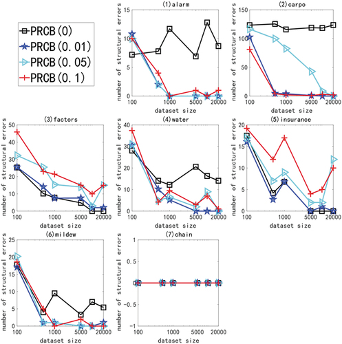
We adopted the above experiment and got a good threshold of 0.01. In the following experiments, the PRCB algorithm is based on this threshold value. For the PRCS algorithm based on significance test, the significance level is selected as 0.005. Then it is compared with KPC, PCB (0.1), Limb, TC (0.005), BESM(0.005), TWO_PHASE and RCS in linear experiment.

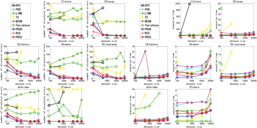
Figure 2 is the result of continuous data of linear multivariate Gaussian distribution generated by ANM<1 > . In two of these figures, the X-axis represents the sample size (100, 500, 1000, 5000, 10000, and 20000), and the Y-axis represents the number of structural errors or the running time. In the experiment, due to the lack of some statistical information and the performance limitation of the algorithm itself, some algorithms can not perform ten-fold cross validation on a specific data set or fail to complete the calculation within 12 hours.

Figure 2. For ANM<1>, the structural errors and running time of the nine algorithms in different networks and data sets.

The following will compare and analyze the PRCB and PRCS algorithms with other algorithms in linear experiments:

The PRCB and PRCS Algorithms and L1MB Algorithm, TC Algorithm, Two-Phase Algorithm and KPC Algorithm in the Linear Experiment

The PRCB and PRCS algorithms have better accuracy and time performance. The L1MB algorithm selects the Markov blanket for each node through the LARS algorithm. This method can describe the correlation between a set of variables and a variable, rather than the correlation between two variables, so this method has certain limitations. The TC algorithm and the Two-Phase algorithm are oriented by identifying the V structure and the orientation algorithm of constraint propagation. There are edges that cannot be oriented. They are treated as structural errors in the experiment, so their accuracy is not very high. The KPC algorithm uses a kernel-based conditional dependency standard for conditional independence test, so the time complexity of the algorithm is particularly high. From the experimental results, the algorithm is only suitable for small samples. On all networks, when the number of samples in the data set is greater than 1000, the running time of the KPC algorithm is greater than 12 hours. In contrast, the algorithm proposed in this article determines the Bayesian network skeleton by directly measuring the conditional correlation between the two variables, and then obtains the final network diagram by the hill-climbing search method. Not only does it not need to spend a lot of time to obtain the Markov blanket for each node, but the resulting network will not have undirected edges, so that its accuracy and time performance are significantly improved compared to the four algorithms.

The PRCB and PRCS Algorithms and the BESM Algorithm, PCB Algorithm and RCS Algorithm in the Linear Experiment

The PRCB algorithm has better accuracy and time performance, while the PRCS algorithm is slightly worse than the three algorithms. PCB algorithm, BESM algorithm and RCS algorithm, respectively, use partial correlation coefficient, linear regression analysis and rank correlation coefficient to measure the independence of variables, and have good structural learning performance, and the three algorithm frameworks are the same as the algorithm framework proposed in this paper. Therefore, the key to determining the performance of the algorithm is the standard used to measure the independence of the variables: partial correlation coefficient and linear regression analysis are both used to test the degree of linear correlation between variables. Partial rank correlation and rank correlation are more inclined to calculate the degree of nonlinear correlation. However, as the number of samples increases, the effects of the methods in the measurement of the degree of linear correlation tend to be the same, and the PCB and BESM algorithms only slightly outperform the PRCS and RCS algorithms when the sample is small. The PRCB algorithm can achieve the best results because the partial rank correlation is calculated based on the converted rank order value, which is more stable than the partial correlation and regression analysis calculated by using the original data, and is not interfered by outliers; second, because it is based on threshold selection, the optimal threshold determined by a large number of experiments makes it more effective in processing small samples than algorithms based on hypothesis testing.

In short, in the linear Gaussian experiment, the partial rank correlation-based causal discovery algorithm PRCB has fewer structural errors than other algorithms, and has achieved better results. The PRCS algorithm based on hypothesis testing shows a moderately upper level in linear experiments, and has a slight disadvantage compared with the optimal algorithm.

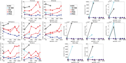
In the nonlinear experiment, we use the multivariate nonlinear non-Gaussian data generated by ANM<2-5> to carry out the experiment. Due to space constraints and consistency of experimental results, only experimental results with ANM<2,3> are presented here. Figures 3 and 4 show the structure error and time performance of the five algorithms, KPC, CD-NOD, RCS, PRCB and PRCS, under different networks and different data sets.

Figure 3. For ANM<2>, the structural error and running time of the five algorithms in different networks and data sets.

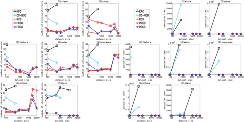
Figure 4. For ANM<3>, the structural error and running time of the five algorithms in different networks and data sets.

The following non-linear result analysis discusses the pros and cons of the PRCB and PRCS algorithms and other algorithms.

PRCB and PRCS Algorithm, KPC Algorithm and CD-NOD Algorithm in Nonlinear Experiments

The PRCB and PRCS algorithm have better accuracy and time performance. The experimental results show that the proposed algorithm has less structural errors and faster computational efficiency on multivariate nonlinear non-Gaussian data. Especially, compared with CD-NOD and KPC algorithms, it has great advantages in processing large sample data sets. Due to the exponential growth of the time required for conditional independence test of these two algorithms, the time efficiency is low for high-dimensional and complex networks and the results cannot be obtained within a limited time. The PRCB and PRCS algorithms only calculate the partial rank correlation coefficient between two variables under the condition of all the remaining variables, which can be quickly obtained by calculating the inverse matrix of the rank correlation coefficient matrix. This simple calculation method not only achieves higher accuracy in all networks, but also handles high-dimensional and complex networks and cases where the number of samples is relatively large.

PRCB and PRCS Algorithm and RCS Algorithm in Nonlinear Experiments

The PRCS algorithm has a slightly higher accuracy, and the PRCB algorithm has a slightly lower performance level. The RCS algorithm uses the rank correlation coefficient to directly test the independence of random variables. Compared with the PRCS algorithm, it only does not consider the joint interference between the variables existing in the multi-complex system. However, due to the small number of nodes in the low-dimensional network and the simple function relationship mentioned above, the joint interference between variables is not obvious. The PRCS algorithm using partial rank correlation has only a slight advantage compared with the RCS algorithm based on rank correlation.

Since the above experiments cannot effectively distinguish the performance of the PRCS algorithm and the RCS algorithm on low-dimensional networks, we hereby conduct mixed function experiments. The result is shown in Figure 5, compared with other algorithms, the PRCS algorithm has better accuracy and time performance. Based on the data generation method of ANM<6>, there are both linear relationships and a large number of non-linear relationships between nodes in the network, and the joint interference between variables in a multivariate system becomes more complicated. In this case, the RCS algorithm, which directly measures the degree of rank correlation between two variables, cannot effectively eliminate interference, and its accuracy is greatly affected. However, the KPC algorithm and the CD-NOD algorithm that perform a large number of conditional independence tests based on the kernel function are not only time-consuming but also not accurate. From the experimental results, the PRCS algorithm that uses the conditional correlation has obvious advantages, and has the least number of structural errors and running time in each network, which confirms the superiority of using partial rank correlation in the multivariate system.

Figure 5. For ANM<6>, the structural error and running time of the five algorithms in different networks and data sets.

In summary, regardless of whether the data is linear or conforms to the Gaussian distribution, the PRCB and PRCS algorithms have high accuracy and time performance. This feature shows that the algorithm has good adaptability. With the advent of the era of big data, algorithms that can process large sample data of high-dimensional networks have more application prospects. For this reason, in addition to conducting experiments on a small sample data set of low-dimensional networks, we conducted the second part of the experiment to explore the performance of algorithms on high-dimensional networks.

Experiment 2: Testing the Performance of the Algorithm on a Large Sample Data Set of High-dimensional Networks

Network and Data Set

To simulate the scenario of high-dimensional features, we created 3 complex networks, as shown in the following table:

Table 5 shows information about three classic high-dimensional networks. The number of nodes is the total number of nodes in the network, and the number of edges is the total number of edges in the network. In the experiment, the data set was generated by the additive noise model. We used the additive noise model ANM with the same six functions as in Experiment 1, and the specific generation method was described above. Based on six data generation modes of ANM and three high-dimensional network structures, network simulation data with sample sizes ranging from 1000 to 1000000 were generated, respectively.

Table 5. Network information

Network	Number of nodes	Number of sides
1 alarm10	370	570
2 hailfinder10	560	1017
3 gene	801	972

Since most of the algorithms tested in the first experiment are dwarfed when dealing with small sample data of low-dimensional networks, their performance will no longer be tested in the second experiment. Although the PRCB algorithm has achieved the best results in the linear experiment of the small network, its performance in the nonlinear experiment is not good. The selection of the significance test threshold of the PRCS algorithm is consistent with the conventional statistical theory, and does not require prior information and expert knowledge. Theoretically, the PRCS algorithm can be applied to different fields and is more universal, and it not only performs well in the nonlinear experiment of small networks, but also shows only a slight disadvantage in the linear experiment. Therefore, we used the PRCS algorithm to carry out the experiments in this part, and the RCS algorithm based on the rank correlation coefficient was used as a reference for comparison experiments. The experimental results adopt the cross-validation method to take the average value after ten times of verification.

Experimental Results and Analysis

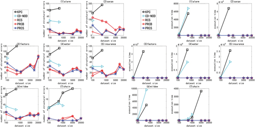
In the experiment of large sample data set of high-dimensional network, we use multivariate linear Gaussian data or nonlinear non-Gaussian data generated by ANM<1-6> to carry out the experiment. Due to space constraints and consistency of experimental results, only experimental results with ANM<1,2,6> are shown here, as shown in Figures 6–8. The X-axis in the figure represents the sample size (1000, 5000, 10000, 100000, and 1000000), and the Y-axis represents the number of structural errors or running time.

Figure 6. For ANM<1>, the structural error and running time of the two algorithms on the high-dimensional network large sample data set.

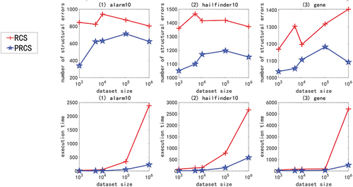
Figure 7. For ANM<2>, the structural error and running time of the two algorithms on the high-dimensional network large sample data set.

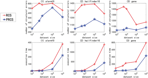
Figure 8. For ANM<6>, the structural error and running time of the two algorithms on the high-dimensional network large sample data set.

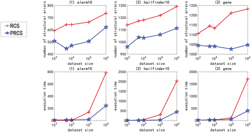
From the above chart data (Table 6), in the experiment of high-dimensional network large sample data set, no matter how the function relationship changes, regardless of the sample size, the PRCS algorithm has extremely significant advantages in terms of structural error and time performance compared to the RCS algorithm. The PRCS algorithm framework is the same as the RCS algorithm framework. PRCS uses conditional correlation and RCS directly measures correlation when measuring the independence of variables. From this we can see that there is a large amount of joint interference between variables in a multi-complex system. It is unreasonable to directly measure the correlation between variables without considering such interference problems, and defects will appear in specific tests. In terms of time performance, the PRCS algorithm for calculating partial rank correlation coefficients should theoretically be higher than the RCS algorithm for calculating rank correlation coefficients, but in reality, as the number of samples increases, the RCS algorithm becomes slower and slower. After repeated reasoning and verification, we came to the conclusion: although in the constraint stage of the algorithm, the RCS algorithm has less time complexity and faster speed, but it does not have obvious advantages. In the search phase of the algorithm, because the RCS algorithm constructs a bad network skeleton, the search is stuck in the local optimum, and it takes a lot of time to get the final network diagram. In contrast to the PRCS algorithm, due to the use of conditionally related partial rank correlation coefficients, the joint interference of multivariate variables can be effectively eliminated, and a good network skeleton can be obtained, so that the causal network diagram can be obtained quickly in the search stage. With this, we once again proved the superiority of the causal structure learning algorithm based on partial rank correlation.

Table 6. Performance comparison of PRCS and RCS on high-dimensional large sample data

Algorithm	Functional relationship	Structural error (Win)	Time performance (Win)
PRCS/RCS	Linear function	3/0	3/0
	Sin function	3/0	3/0
	Power function	3/0	3/0
	Cos function	3/0	3/0
	Exponential function	3/0	3/0
	Mixed function	3/0	3/0

Next, we specifically analyze the structural error and execution time of the PRCS algorithm on the high-dimensional network. In terms of time, even if the data dimension increases, the time of the PRCS algorithm still increases linearly. In the above experiment, even if it processes one million data sets generated by the largest gene network, it takes only 400s to 500s. Compared with the huge data stream and high-dimensional features, the time performance is very impressive. In terms of the number of network structure errors, by calculating the total number of network structure edges of each network, we can get: 136900 (alarm10), 313600 (hailfinder10) and 641601 (gene), corresponding to the average number of errors for each network on a million data sets: 593.05 (alarm10), 1099.58 (hailfinder10) and 1067.37 (gene). We can find that relative to the huge data stream and high-dimensional features, the network structure error rate is less than 1%, indicating that the PRCS algorithm maintains a good accuracy rate and can effectively solve the problem of causal discovery on high-dimensional large sample data sets.

In summary, we can think that the PRCS algorithm is suitable for scenarios with arbitrary data distribution, arbitrary network structure, and high-dimensional large samples, and can achieve good results. The two-part experiment proves that the PRCS algorithm can better dig out the hidden causal relationship in the data set and restore the causal network diagram. It lays the experimental and theoretical basis for the application of the following causal structure learning algorithm based on partial rank correlation in the power plant measuring point fault prediction system.

Experiment 3: Application of the Algorithm on Real Data Sets

Power Plant Measuring Point Data Set

The data used in the experiment are collected from the sensor data of the measuring points recorded in a power plant in 2020. The data recorded 520 points between 1–1 and 2020-3-24. The equipment was collected every 30 seconds, generating an average of 60,480 pieces of data per week. The physical significance of some measuring points is shown in Table 7.

Table 7. Some sensor measuring point information of a power plant

Measuring point number	Measuring point	Unit
1	Unit load	MW
2	A side steam turbine inlet steam temperature	°C
3	Inlet steam temperature of A side medium pressure main valve	°C
4	A side cold re-steam temperature	°C
5	First extraction steam temperature	°C
6	Second extraction steam temperature	°C
7	Six extraction steam temperature	°C
8	Low pressure exhaust steam temperature (motor end)	°C
9	Low pressure exhaust steam temperature (valve end)	°C
10	1# bearing metal temperature (right side)	°C
11	2# bearing metal temperature (left side)	°C
12	Speed 1#	r/min
13	Rotor eccentric	%
14	Axial displacement 1	um
15	Differential expansion	um
16	2#Bearing vibration	um
17	Six-stage extraction steam pressure	MPa
18	Main steam flow	t/h

Obviously, derived from the real production environment of power plant data with high dimension, the data quantity is large and frequent fluctuations of continuous characteristics of conventional methods to prevent equipment failure from the data, also can’t when the equipment failure by detecting data changes quickly determine the fault point, and after the failure is difficult to obtain effective mechanism of information to put an end to the same kind of the cause of the problem. Therefore, we will use the PRCS algorithm to build the causal network structure of the data, to find out the potential causality between the test points, so as to effectively predict the operation status of the test points, and provide a strong basis for fault detection and fault prevention in power plants.

Causal Fault Detection System Based on Partial Rank Correlation

Based on the above, we propose a fault detection system as shown in Figure 9. The system is divided into three stages. The first stage: It is used to realize the network structure learning based on the input power plant measuring point data set, and obtain possible candidate neighbor measuring points (TCN) for each measuring point data. At this stage, for each input measuring point data $X_j$, $\mathrm{T}\mathrm{C}\mathrm{N}\left(X_j\right)$ are initialized to empty. For each other measuring point $X_j$, $\mathrm{T}\mathrm{C}\mathrm{N}\left(X_j\right)$ is obtained by calculating $DEP\left(X_i,X_j\right)$ ($DEP\left(X_i,X_j\right)=p-value\left(X_i,X_j\right)$, the calculation method of p-value is described in section 4.2). If $DEP\left(X_i,X_j\right)$ is less than a certain significance detection threshold, $X_i$ is added to $\mathrm{T}\mathrm{C}\mathrm{N}\left(X_j\right)$, and based on symmetry, $X_j$ is also added to $\mathrm{T}\mathrm{C}\mathrm{N}\left(X_i\right)$.

Figure 9. Flow chart of causal fault detection system based on partial rank correlation.

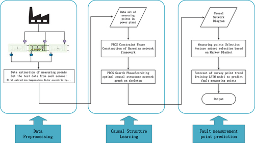
The second stage: Perform a score search on the Bayesian network structure skeleton obtained in the first stage, and use a restricted greedy search method to obtain the final causal structure network diagram.

The third stage: feature selection based on the causal structure network diagram, and a reduced subset is obtained by selecting the measurement points directly related to the current measurement point prediction (the selection conditions of the measurement points are based on prior knowledge such as Markov blanket). The subset of measurement points is input into the deep learning model for training to obtain a model that meets the requirements, and the model is used to predict the trend of the current measurement point.

Experimental Results and Analysis

In the experiment, we can obtain the causal network structure diagram of each measuring point in the power plant. Due to the large number of measuring points, only part of the causal network structure diagram is shown here.

As shown in Figure 10, some measuring points have inter-causality or indirect causality, while isolated nodes in the figure (without arrows pointing or pointing out) indicate that data changes of the measuring points themselves are not affected by other measuring points, that is, there is no causal relationship. From the data, these isolated measuring points are constant values and do not change with time. Therefore, the causal network diagram is very consistent with the actual measuring point state according to the combined data.

Figure 10. Part of the causality diagram of a measuring point in a power plant.

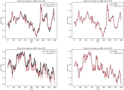
After obtaining the network diagram reflecting the causality relationship between the measured points, we trained the prediction model of the target measured points to verify the accuracy and effectiveness of the causality analysis. The experiment uses the long – short – term memory network LSTM as a prediction model. The data from January 7 to 13 of 20 years were selected as the training data, and the data from January 14 was selected as the test data. In order to better illustrate the reliability of the causality diagram constructed by the PRCS algorithm and the superior performance of the fault detection system based on this design, we use all the measuring points to predict the trend of the current measuring points, and make a contrast experiment with the prediction of the current measuring points based on the relevant measuring points selected by the PRCS algorithm. The results are shown in the following figure

As can be seen from Figure 11, the original data of each measuring point in the power plant has a complex nonlinear mapping relationship, and the mechanism relationship is also particularly complex. If all measuring points are used to predict the current trend of measuring points, the results will be somewhat different from the actual data. However, the fault detection system we designed is based on the causal network diagram constructed by the PRCS algorithm. After feature selection, we find the directly related measurement points of each measurement point from the original data of the non-linear and irregular state. Then predict based on the selected subset of measurement points, and the obtained predicted trend basically fits the real trend data of the current measurement point. The model prediction results of the above five measuring points (2,42,106,210,325) show that our PRCS algorithm can effectively remove the influence of irrelevant measuring points on observation measuring points. This proves that the causal fault detection system based on partial rank correlation has good detection performance.

Figure 11. Experimental results of power plant fault measurement points prediction.

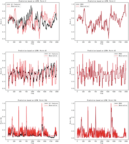
Figure 11. Continued.

By referring to the data and conducting common mechanism analysis, it can be concluded that the causality diagram of measuring points in Figure 10 is relatively consistent with the mechanism analysis. The causality relationship obtained based on the algorithm will help us to better predict and diagnose the fault model. Therefore, we can draw the conclusion that the causal discovery algorithm model based on partial rank correlation can effectively identify the nonlinear causal relationship of multivariate systems, remove the influence of redundant variables well, and have excellent learning ability of causal network structure, which is more competitive than similar algorithms. The fault detection system designed by this algorithm can not only monitor each measuring point in real time before the power plant failure, but also help the maintenance personnel to quickly determine the cause of the failure and repair the measuring point when the power plant failure occurs. And through the study of the corresponding causal network structure, we can reveal some hidden mechanisms that have not been discovered so far, so that the products with better performance are expected to achieve a wide range of application prospects.

Conclusion

The problem of causal discovery in the era of big data is a topic worthy of in-depth exploration. In this article, by studying the partial rank correlation coefficient and its application in additive noise models, we propose two novel causal structure learning algorithms based on partial rank correlation – PRCB and PRCS algorithms. First, we prove that the partial rank correlation coefficient can be used as a measure of independence, and redefine the correlation between variables in a multivariate system from the perspective of partial rank correlation. Second, by applying partial rank correlation to Bayesian network structure learning, a PRCB algorithm based on threshold selection is proposed. However, the optimal threshold of the PRCB algorithm requires prior knowledge and a large number of experiments to obtain. We further introduced statistical hypothesis testing methods to solve such defects, and proposed a PRCS algorithm based on hypothesis testing. Finally, with the help of theoretical analysis and a large number of experiments, it is verified that the proposed algorithm can not only effectively deal with the causal structure learning problem of linear Gaussian or nonlinear non-Gaussian data on low-dimensional networks, but also can efficiently deal with the analysis of large sample data sets on high-dimensional networks. The results show that the causal structure learning algorithm based on partial rank correlation not only has a reliable theoretical basis, but also has extremely high accuracy and efficient time performance, and it has a good algorithmic competitiveness. And the causal fault detection system designed based on this algorithm has proved its superior performance in experiments. It can build a Bayesian network diagram by mining data causality, thereby predicting the trend of fault measurement points, and assisting the fault prevention and fault maintenance of power plant equipment, and has a good application prospect.

In future research, we will further explore the application research of the algorithm in additive noise models, and the proposed algorithm is used to detect and isolate faults in sensor systems (Darvishi et al. 2020). Theoretically, the algorithm framework proposed in this paper has strong transferability, and can also be applied to financial stock trend prediction and medical image processing tasks.

Disclosure Statement

No potential conflict of interest was reported by the author(s).

Additional information

Funding

This work was supported by the Anhui Province Key Research and Development Plan (No. 201904a05020073), the National Key Research and Development Program of China (No. 2020AAA0106100), the National Natural Science Foundation of China (No. 61876206, 71771203, 61872327 and 61902068), Guangdong Basic and Applied Basic Research Foundation (No. 2020A1515011499);the Anhui Province Key Research and Development Plan;

Appendices

Acronym

Table

BESM	Based on simultaneous equations model
CB	CI test based methods and Bayesian methods
CS-NOD	Constraint-based causal Discovery from Nonstationary/heterogeneous Data
HSIC	Hilbert-Schmidt-Independence-Criterion
KCI	Kernel-based-Conditional-Independence
KPC	Kernel-PC
L1MB	L1-regularized-Markov-Blanket
LSMI	Least-Squares-Mutual-Information
MMHC	Max-Min-Hill-Climbing
PCB/PCS	Partial-Correlation-Based/Partial-Correlation-Statistic
PRCB/PRCS	Partial-Rank-Correlation-Based/Partial-Rank-Correlation-Statistics
RCS	Rank-Correlation-Based

Appendix

Related work comparison table

Table

Multiple Linear Causal Discovery Algorithm	Multivariate Nonlinear Causal Discovery Algorithm
L1MB Algorithm	HSIC conditional independence test
TC Algorithm	MAP (Maximum A Posteriori)
Two-Phase Algorithm	KPC Algorithm
PCB/PCS Algorithm	CS-NOD Algorithm
PRCB/PRCS Algorithm

Appendix

Statistical Distribution Properties of Partial Rank Correlation Coefficients

Theorem 4.1: For the data generated by the additive noise model, the disturbances conform to an arbitrary distribution and are not correlated with each other. V is the variable set, m is the number of samples, n is the number of variables, and m is large enough. $\mathrm{\forall }{X}_i$, $X_j\in \mathbf{V}$,, $\mathrm{P}\mathrm{N}(X_j)=\mathrm{\varnothing }$ partial rank coefficient ${\rho }_r\left(X_i,X_j|\mathbf{Z}\right)$, abbreviated as ${\rho }_{ij}$, regardless of whether the data conforms to the multivariate normal distribution, the distribution of the statistic T approximately obeys the student t distribution with m-n degrees of freedom.

$T=\frac{{\rho }_{ij}}{\sqrt{\left(1-{\rho }_{ij}^2\right)/\left(m-n\right)}}$

Proof: First of all, the following theorems 1, 2, 3 can be obtained by looking up the information. For the data generated by the additive noise model, if the disturbance conforms to the normal distribution, the data set obeys the multivariate normal distribution. $\mathrm{\forall }{X}_i$, $X_j\in \mathbf{V}$, $\mathbf{Z}\subseteq \mathbf{V}\mathrm{\setminus }\left\{X_i,X_j\right\}$, the order of the partial rank correlation coefficient ${\rho }_{ij}$ is n-2, then applying theorem 1 and theorem 3, we can get that T obeys the student t distribution with m-n degrees of freedom. For the data generated by the additive noise model, if the disturbance does not conform to the normal distribution, the data set does not obey the multivariate normal distribution. According to theorem 2, even if the data is non-normal, as long as the sample is not very small, the statistic t₁ approximately obeys the student t distribution with m-2 degrees of freedom. According to theorem 3, the sampling distribution of partial rank correlation coefficient is the same as that of rank correlation coefficient, so it can be obtained that T obeys the student t distribution with m-n degrees of freedom, and the theorem is proved.

Theorem 1: If the variable has a bivariate normal distribution, and ${\mathrm{r}}_{ij}$ represents the Spearman rank correlation coefficient between the variables $X_i$ and $X_j$, then the t₁ distribution of the rank correlation coefficient statistics obeys the student t distribution with m-2 degrees of freedom, m is the sample size, which is

$t_1=\frac{r_{ij}}{\sqrt{\left(1-r_{ij}^2\right)/\left(m-2\right)}}$

Theorem 2: Even if the data is non-normal, theorem 1 is approximately true when the number of samples is not very small.

Theorem 3: Let ${\rho }_{ij.k}$ denote the partial rank correlation coefficient of order k. Under the non-zero hypothesis, the sampling distribution of ${\rho }_{ij.k}$ is the same as the distribution of ${\mathrm{r}}_{ij}$, and the statistic t₂ obeys the student t distribution with m-2-k degrees of freedom.

$t_2=\frac{{\rho }_{ij.k}}{\sqrt{\left(1-{\rho }_{ij.k}^2\right)/\left(m-k-2\right)}}$

References

- Chen, W., R. Cai, K. Zhang, Z. J. I. T. O. N. N. Hao, and L. Systems. 2021. Causal discovery in linear non-Gaussian acyclic model with multiple latent confounders. IEEE Transactions on Neural Networks and Learning Systems 1–1695. doi:10.1109/TNNLS.2020.3045812.
- Conover, W. J. 1998. Practical nonparametric statistics, vol. 350. John Wiley & Sons.
- Cooper, G. F., and E. J. M. L. Herskovits. 1992. A Bayesian method for the induction of probabilistic networks from data. Machine learning . 9 (4):309–47.
- Darvishi, H., D. Ciuonzo, E. R. Eide, and P. S. J. I. S. J. Rossi. 2020. Sensor-fault detection, isolation and accommodation for digital twins via modular data-driven architecture. IEEE Sensors Journal . 21 (4):4827–38.
- Duggento, A., M. Guerrisi, and N. Toschi. 2019. Recurrent neural networks for reconstructing complex directed brain connectivity. Paper presented at the 2019 41st Annual International Conference of the IEEE Engineering in Medicine and Biology Society (EMBC). Berlin, Germany.
- Fieller, E. C., H. O. Hartley, and E. S. J. B. Pearson. 1957. Tests for rank correlation coefficients. I. Biometrika . 44 (3/4):470–81.
- Foraita, R., J. Friemel, K. Günther, T. Behrens, J. Bullerdiek, R. Nimzyk, … V. J. J. O. T. R. S. S. S. A. Didelez. 2020. Causal discovery of gene regulation with incomplete data. Journal of the Royal Statistical Society: Series A (Statistics in Society). 183 (4):1747–75.
- Friedman, N., I. Nachman, and D. J. Pe’er. 2013. Learning Bayesian network structure from massive datasets: The” sparse candidate” algorithm. arXiv preprint arXiv: 1301.6696 .
- Fukumizu, K., A. Gretton, X. Sun, and B. Schölkopf. 2007. Kernel measures of conditional dependence. Paper presented at the NIPS. Vancouver, British Columbia, Canada.
- Gretton, A., R. Herbrich, and A. J. Smola. 2003. The kernel mutual information. Paper presented at the 2003 IEEE International Conference on Acoustics, Speech, and Signal Processing, 2003. Proceedings.(ICASSP’03), Hong Kong, China.
- Kleijnen, J. P., J. C. J. R. E. Helton, and S. Safety. 1999. Statistical analyses of scatterplots to identify important factors in large-scale simulations, 1. Review and Comparison of Techniques 65 (2):147–85.
- Mazlack, L. J. 2009. General causal representations in the medical domain. Paper presented at the 2009 2nd International Conference on Biomedical Engineering and Informatics. Tianjin, China.
- Mooij, J., D. Janzing, J. Peters, and B. Schölkopf. 2009. Regression by dependence minimization and its application to causal inference in additive noise models. Paper presented at the Proceedings of the 26th annual international conference on machine learning. Montreal, Quebec, Canada.
- Onan, A., and M. A. J. I. A. Toçoğlu. 2021. A term weighted neural language model and stacked bidirectional LSTM based framework for sarcasm identification. IEEE Access. 9:7701–22.
- Onan, A., and S. J. J. O. I. S. Korukoğlu. 2017. A feature selection model based on genetic rank aggregation for text sentiment classification. Journal of Information Science. 43 (1):25–38.
- Onan, A., S. Korukoğlu, and H. J. E. S. W. A. Bulut. 2016. A multiobjective weighted voting ensemble classifier based on differential evolution algorithm for text sentiment classification. Expert Systems with Applications. 62:1–16.
- Pearl, J. 2014. Probabilistic reasoning in intelligent systems: Networks of plausible inference. Morgan kaufmann, Elsevier.
- Pellet, J.-P., A. J. I. Elisseeff, N. Y. North Castle, and U. S. A. Research. 2007. Partial correlation and regression-based approaches to causal structure learning. IBM, North Castle, NY, USA, Research.
- Pellet, J.-P., and A. J. J. O. M. L. R. Elisseeff. 2008. Using Markov blankets for causal structure learning. Journal of Machine Learning Research. 9 (7).
- Schmidt, M., A. Niculescu-Mizil, and K. Murphy. 2007. Learning graphical model structure using L1-regularization paths. Paper presented at the AAAI. Vancouver, British Columbia, Canada.
- Singh, M., and M. Valtorta. 1993. An algorithm for the construction of Bayesian network structures from data. Paper presented at the Uncertainty in Artificial Intelligence. Washington, DC.
- Spirtes, P., C. Glymour, and R. Scheines. 1989. Causality from probability.
- Tillman, R. E., A. Gretton, and P. Spirtes. 2009. Nonlinear directed acyclic structure learning with weakly additive noise models. Paper presented at the NIPS. Vancouver, BC, Canada.
- Tsamardinos, I., L. E. Brown, and C. F. J. M. L. Aliferis. 2006. The max-min hill-climbing Bayesian network structure learning algorithm. Hormone Research 65 (1):31–78. doi:10.1159/000090377.
- Wang, Z., and L. Chan. 2010. An efficient causal discovery algorithm for linear models. Paper presented at the Proceedings of the 16th ACM SIGKDD international conference on Knowledge discovery and data mining. Washington, DC, USA.
- Wu, P., and K. Fukumizu. 2020. Causal mosaic: Cause-effect inference via nonlinear ica and ensemble method. Paper presented at the International Conference on Artificial Intelligence and Statistics. Palermo, Sicily, Italy.
- Yamada, M., L. Sigal, M. Raptis, M. Toyoda, Y. Chang, M. J. I. T. O. P. A. Sugiyama, and M. Intelligence. 2015. Cross-domain matching with squared-loss mutual information. IEEE Transactions on Pattern Analysis and Machine Intelligence 37 (9):1764–76. doi:10.1109/TPAMI.2014.2388235.
- Yamada, M., and M. Sugiyama. 2010. Dependence minimizing regression with model selection for non-linear causal inference under non-Gaussian noise. Paper presented at the Twenty-Fourth AAAI Conference on Artificial Intelligence. Westin Peachtree Plaza in Atlanta, Georgia, USA.
- Yang, J., G. Fan, K. Xie, Q. Chen, and A. J. I. S. Wang. 2021. Additive noise model structure learning based on rank correlation. Information Sciences, 571:499–526.
- Yang, J., L. Li, and A. J. K.-B. S. Wang. 2011. A partial correlation-based Bayesian network structure learning algorithm under linear SEM. Knowledge-Based Systems. 24 (7):963–76.
- Yang, J., N. An, G. J. I. T. O. K. Alterovitz, and D. Engineering. 2016. A partial correlation statistic structure learning algorithm under linear structural equation models. IEEE Transactions on Knowledge and Data Engineering. 28 (10):2552–65.
- Zeng, Y., Z. Hao, R. Cai, F. Xie, L. Huang, S. J. I. T. O. N. N. Shimizu, and L. Systems. 2021. Nonlinear causal discovery for high-dimensional deterministic data.
- Zhang, K., B. Huang, J. Zhang, C. Glymour, and B. Schölkopf. 2017. Causal discovery from nonstationary/heterogeneous data: Skeleton estimation and orientation determination. Paper presented at the IJCAI: Proceedings of the Conference. Melbourne, Australia.
- Zhang, K., J. Peters, D. Janzing, and B. J. A. P. A. Schölkopf. 2012. Kernel-based conditional Independence test and application in causal discovery. arXiv preprint arXiv: 1202.3775.