Artificial Intelligence Aided Agricultural Sensors for Plant Frostbite Protection

ABSTRACT

Frostbite and frost is one of the problems that endanger the health of crops and can ruin plants and fruits. Soil temperature is the most significant factor that influences the freezing depth. Therefore, monitoring and predicting this characteristic is crucial for frostbite protection. This study aims to predict soil temperature on cold days to prevent frostbite injury in crops. For this matter, we used the registered and logged hourly data by the HOBO U30 data logging device and predicted the soil temperature from air temperature, soil water content, and relative humidity. We used 80% of the data set for the training data and assigned the other 20% to the test data. RMSE and MSE were two of the evaluation criteria of the neural network in this study. Also, we calculated P-value and T-value for statistical hypothesis testing. In another approach for weighting the neural network, we used evolutionary algorithms such as Genetic Algorithm and Particle Swarm Optimization instead of the gradient-based methods. According to the results, Multi-layer perceptron neural network with the respective values 0.082 and 0.0068 for RMSE and MSE in training data and 0.085 and 0.0073 for RMSE and MSE in testing data proved to have a better performance in the soil temperature prediction compared to the ANN-GA and ANN-PSO models. Farmers, botanical researchers, and policymakers in food security can use these results.

Introduction

Frostbite is one of the most critical agricultural problems globally, affecting plant growth and crop yield, causing substantial crops losses (Taheri, Tarighi, and Taheri 2014). Cold weather may occur in more than 93% of the world, and 81% of these areas are prone to frost (Nilsen and Orcutt 1996; Steponkus, Uemura, and Webb 1993). In many countries with dry climate, frost causes food deficiencies and financial losses. Due to agricultural damages caused by frost in Australia, financial losses have been predicted to be hundreds of millions of dollars. Besides the straightforward injuries from frost in the grains group, the same or higher costs are incurred by farmers utilizing conservative methods like planting later than ideal for eschewing frost (Gobbett et al. 2021). Wheat is the third-biggest crop globally, with an annual production of more than 600 million tons. Severe weather conditions, like frost (less than 0◦C) and heat shock (greater than 33◦C), affect crops yields and represent a substantial danger that requires to be administered. When Frost occurs during reproductive and vegetative growth, it can affect seedling survival rate from medium to extreme (Barlow et al. 2015). Reports in December 2018 represented rising frost injury to many trees in vast areas of Central Europe due to global warming (Ding, Noborio, and Shibuya 2019). Fresh Plaza is a website that shares many news and articles on a global scale in agriculture. Also, on this website, information about economic losses due to frost injuries and the anxiety of people in southern Europe about frost injury to stone fruit can be accessible (https://www.freshplaza.com). Agriculture has a critical role in the economic activities of the world. To control the quality of agricultural products, it is essential to understand the various factors that impact the well-being of these products. Frost event is impacted by climatic conditions, topography, land orientation, soil condition, and etc (Cadenas et al. 2020). Soil acts as energy storage during the day and a heat source overnight. The energy stored on warm days of the year is released when the weather is cold (Atkinson 2003). The soil temperature is an essential parameter in agricultural meteorology (Araghi et al. 2017) and has a crucial function in the climate system due to changing soil hydrological and thermic characteristics; for instance, frozen soil affects the snowmelt and diminishes the soil coefficient of permeability (Mohammadi, Moghbel, and Ranjbar 2016) Moreover, the researchers have reported that soil temperature changes influence plant growth in essential steps (like germination and seedling emergence) and plant root growth. In fact, increments in soil temperature improve the root growth of plants due to the increment in metabolic action at root cells and the expansion of plant tissue nutrients. Also, soil temperature directly affects physiological, chemical, and biological soil activity and causes decomposition of soil organic matter and release of Carbon dioxide (CO2) (Paul et al. 2004). In soil heat physics, the soil temperature depends on several properties, consisting meteorological conditions (like air temperature and air temperature), soil physical variables (like texture and water content), topographical parameters (like slope and elevation), and surface characteristics (like ground litter stores and leaf area index). Evidence shows that forecasting spatial and temporal models of soil temperature enhances our knowledge about the dynamics of soil vegetation (Kang et al. 2000). In addition to these, the temperature of soil influences soil water maintenance, transportation, and plant access to it. Therefore, if the soil temperature is outside a proper range, agricultural losses occur. Consequently, soil temperature influences crop growth and function more significantly than the air temperature and plants leaf temperature (Araghi et al. 2017) and it can help predict the cold and estimate the severity of frostbite damages to agricultural products. Precision agriculture, with related technologies, has appeared as a field that uses data collection methods and machine learning models to control agriculture productivity. Different types of environmental sensors are utilized in this technology to gather information on crop products, climatic and soil conditions. These are as follows: pH sensor, humidity sensor, temperature sensor, location sensors, optical sensors, electrochemical sensors, mechanical sensors, dielectric soil moisture sensors, and airflow sensors. This information allows an excellent knowledge of the environment and will provide quicker, more effective and robust decision-making systems (Liakos et al. 2018).

The goal of this study is to predict the degree of soil temperature in the cold days of the year based on sensor readings in previous days. The rest of this paper is structured as follows. Section II reviews previous related work. Section III describes the environment and methods used for this study. Section IV briefly explains neural networks. Section V elaborates on the proposed algorithm. Finally, Sections VI, VII, and VIII are results, discussion, and conclusion, respectively.

Previous Work

Soil organic carbon increases the potential and actual soil power for producing rich products and is a key index for sustainable agriculture. This feature of the soil caught the attention of Kennedy Were in 2015 and laid the foundation for a study for the purpose of predicting soil organic carbon in the soil (Were et al. 2015). These researchers evaluated random forest (RF), artificial neural network (ANN), and support vector machine (SVM) methods for regression in their study. Among the nutritional elements, phosphorous is the most important factor for plant growth and soil fertility after nitrogen. This element is involved in all biochemical processes and in energy transfer mechanisms. In (Keshavarzi et al. 2015), a team lead by Ali Keshavarzi was formed for predicting the amount of phosphorous using a neural network. The saturated hydraulic conductivity of the soil (K_s) is one of the most important physical characteristics of the soil and has a significant effect on the infiltration of water in the soil and controlling the surface pollution with groundwater. Kourosh Ghaderi et al. have proposed group method of data handling and harmony search (GMDH-HS) for estimating the value of K_s in (Qaderi et al. 2018). Ali Asghar Vahedi has conducted research with the goal of monitoring the available carbon in forest soil (Vahedi 2017). Forest soil has more carbon compared to the soil of other regions and has an important role in the carbon production cycle. The proposed method in this study was the multi-layer perceptron neural network. Organic agriculture or sustainable agriculture can be defined in its simplest form as “Agriculture without adding chemical and industrial material.” Soil water content is one the most important factors that affect the implementation of sustainable agriculture. Chatterjee et al (Chatterjee, Dey, and Sen 2018) proposed a scheme for predicting the amount of soil water content using a neural network. They used the modified flower pollination algorithm (MFPA) optimization method for training the weights of the neural network instead of the conventional standard gradient-based methods. The goal of research in (Nosratabadi et al. 2020) was to present a machine learning approach with high predictive accuracy for crop yield prediction. For this purpose, artificial neural networks-gray wolf optimizer (ANN-GWO) and artificial neural networks-imperialist competitive algorithm (ANN-ICA) were selected and evaluated. The result concludes that ANN-GWO has a better performance in the crop yield prediction than the ANN-ICA model. In (Ardabili et al. 2019) the authors introduced a predictive model for temperature variation of the mushroom growing hall. For this purpose, Multi-layered perceptron (MLP) and radial basis function (RBF) networks as candidate methods were selected. Water temperature, ambient temperature, circulation air dampers, fresh air, and water tap were taken as independent variables. This study was performed with three steps. The first step was data processing. The second and third steps were implementing MLP and RBF and obtaining results, respectively. Results showed that RBF offers better efficiency and performance than MLP. Researchers in (Nosratabadi et al. 2021) used two machine learning models for the prediction of food production. These models were multilayer perceptron (MLP) and adaptive network-based fuzzy inference system (ANFIS). The performance of MLP and ANFIS methods was evaluated utilizing time-series data of agricultural and livestock products. Two variables of livestock and agricultural production for the source of food production was used. According to the results, ANFIS has high predictive precision in the crop yield prediction than MLP.

Materials and Methods

Describing the Test Site

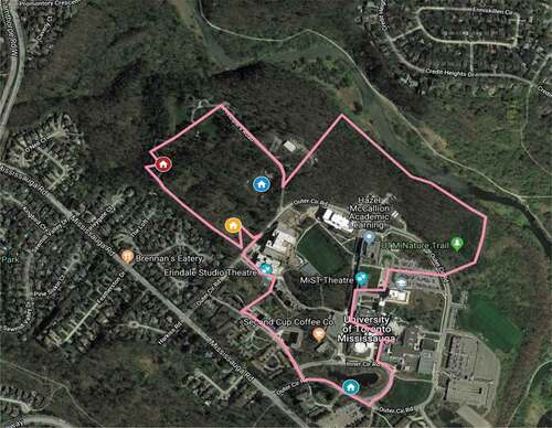
Toronto is the provincial capital of Ontario and is the largest city of Canada. This city is positioned in southern Ontario region and in the northwest of Ontario Lake. Toronto has a semi-continental climate and cold winters and warm and humid summers. Although, Toronto’s weather in winter is warmer than the rest of the cities, it still has rough winters and the ground is covered with snow from mid-December until mid-March. Figure 1 shows the geographical location of our test site in this study. This location is placed near the University of Toronto.

Figure 1. The geographical location of this study.

Gathering Field Information

The input information in this study is air temperature, soil water content, and relative humidity and our goal is to predict the soil temperature from these input characteristics. The dataset used in this study is accessible in (https://www.utm.utoronto.ca/geography/resources/environmental-datasets). The information within this dataset is gathered hourly from a farm in the University of Toronto by an electronic device named HOBO U30 data logger. HOBO U30 data logging device has environmental sensors for gathering information and internal storage to save them (Figure 2). The information gathered by these devices is sent to the base station every 24 hours and can be received at the end of the month via the website address mentioned earlier. We used the information from the first quarter of 2018 in our study.

Figure 2. The installation of the HOBO U30 data logger device (https://www.utm.utoronto.ca/geography/resources/environmental-datasets).

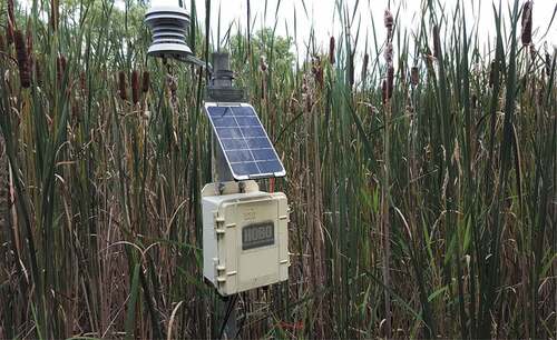
Figure 3. HOBO U30 components (https://www.onsetcomp.com).

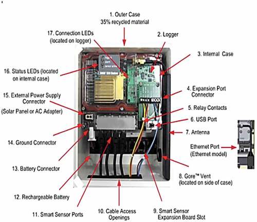
Smart sensors connect into the logger and gather data about different parameters. HOBO-U30 can connect up to 10 smart sensors of any model or combination. Components of HOBO U30 shown in Figure 3 are (https://www.onsetcomp.com):

• Outer Case

• Logger

• Internal Case

• Development Port Connector

• Relay Contacts

• USB Port

• Antenna or Ethernet Port

• Vent

• Smart Sensor Development Slot

• Cable access openings

• Smart Sensor Ports

• Rechargeable Battery

• Battery Connector

• Ground Connector

• External Power Supply Connector

• Status LEDs

• Connection LEDs

The Features of Input Characteristics

According to the researchers in (Wu and Nofziger 1999), air temperature is among the effective factors of daily and annual changes in soil temperature. Humidity is also counted as one of the reasons of temperature loss in the soil profile. The amount of heat loss increases with soil water content. The heat flow in humid soil is more than that of dry soil whose pores are filled with air. Humid loss occurs when an increase in soil temperature causes the water to lose its viscosity. The loss of shadow along with the increase in soil temperature leads to more evaporation which limits the movement of water in soil. The existing water in soil is evaporated by the sunlight radiation and the soil temperature will be colder as the evaporation speed increases (Atkinson 2003; Ochsner, Horton, and Ren 2001).

Neural Network

Inspired by the units of the neural systems the artificial neural network has become a handy tool in artificial intelligence (Maren and Harston 2014; Liu, Zhu, and Cao 2017; Varol, Canakci, and Ozsahin 2015). Figure 4 shows the structure of a neural network.

Figure 4. The structure of the artificial neural network (Heidari and Shamsi 2019).

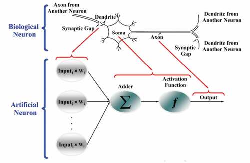
Various topologies exist for modeling the artificial neural network among which multi-layer perceptron (MLP) neural network, single-layer perceptron (SLP) neural network, and feed-forward based on back-propagation (FF-BP) neural network can be mentioned. Among these topologies, MLP is one of the neural network models that has been variously for solving different problems. MLP neural network is composed of three layers named input layer, hidden layer, and output later in which neurons are grouped. Figures 5 and 6 show the feed-forward neural structure and the structure of a neuron in a feed-forward neural network.

Figure 5. Feed-forward neural network (Fath, Madanifar, and Abbasi 2020).

Figure 6. The structure of a neuron in a feed-forward neural network (Messikh, Bousba, and Bougdah 2017).

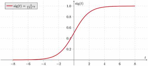
Figure 7. The sigmoid activation function (https://www.onsetcomp.com).

Equation 1 mathematically shows how the neural network is trained:

(1) $Y=f\left(\sum _{i=1}^n{w}_i{X}_i+b\right)$(1)

In the formula above, $X_i$ is the set of inputs with n components. b and $w_i$ represent the bias and weight of the neurons, respectively. The function, f, which is referred to as activation function. In this paper, we chose it to be the sigmoid function shown in Figure 7.

The Proposed Model for the Neural Network

We have used the two-layer perceptron neural network to predict the soil temperature from the characteristics of air temperature, relative humidity, and soil water content. The number of neurons selected for each layer depends on the type of problem. But if the number is too high, the network will be overfitted. We have chosen 5 neurons for the hidden layers of the neural network. In order to design an artificial neural network, a huge dataset is required for the input and output layers. In the dataset used for this study, 2216 entries were reported for each characteristic. In total, 8864 samples exist in this dataset and we have used 80% of the input data for the training section and other 20% was assigned to the test section. The network can learn the training pattern by changing the weights. We have used the Levenberg-Marquardt learning algorithm for updating the weights and the bias value in the proposed model for MLP. The activation function is the sigmoid function.

We have obtained statistical descriptive indices for the input characteristics in this study i.e. soil water content, relative humidity, and air temperature whose values are shown in Table 1. These indices are classified into three groups named central tendency indices, variation indices, and distribution symmetry indices. The median and mean show how much the data is centered and are called central tendency parameters. The coefficient of variation and variance show the changes and variation of data. Equation (2)(2) $Cv\left(\mathrm{\%}\right)=\frac{\sigma }{\mu }$(2) shows the mathematical relation for the coefficient of variation

(2) $Cv\left(\mathrm{\%}\right)=\frac{\sigma }{\mu }$(2)

Table 1. The statistical characteristics of air temperature, soil water content, and relative humidity

Variable	Air_temp	Soil_wc	rh
Min	−25.38	0.08	26.3
Max	16.2	0.22	100
Mean	−2.09	0.13	75.12
Median	−1.69	0.12	77.3
Skewness	−0.43	0.719	−0.6268
Kurtosis	3.7	2.35	2.85
Variance	43.05	0.001	268.09
CV%	−314.29	24.32	21.79

In the formula above, $\sigma$ and $\mu$ represent the variance and mean, respectively.

Skewness and kurtosis are the distribution symmetry indices and show the amount of horizontal and vertical asymmetry with respect to the standard normal distribution curve respectively. We have used root mean square error (RMSE) and mean square error (MSE) to evaluate the prediction accuracy of soil temperature and their relations are shown in (3) and (4):

(3) $MSE=\frac{1}{n}\sum _{i=1}^n{\left(y_P\left(i\right)-y_o\left(i\right)\right)}^2$(3)

(4) $RMSE=\sqrt{\frac{1}{n}\sum _{i=1}^n{\left(y_P\left(i\right)-y_o\left(i\right)\right)}^2}$(4)

In Equations (3) and (4), $y_P\left(i\right)$ is the output value predicted by artificial intelligence and $y_o\left(i\right)$ is the real output value.

In inferential statistics, statistical hypothesis testing is one of the most important and conventional methods. This test has been used in this study to guarantee the quality of the experiment results. Tor this purpose, the values for p-value and T-value are calculated. Null-hypothesis is usually an opinion about the parameter or the statistical population which had already existed and our goal is to reject the null hypothesis. Rejecting null-hypothesis means that our findings were statistically meaningful. The accuracy or error rate of voting for the rejection of null-hypothesis is called significance level which was assigned to 95% in this study. The significance level shows how much the maximum error was while rejecting the null-hypothesis. In addition to the parameters above, confidence interval, degree of freedom, and the mean are also obtained for the target variable. The confidence interval is a kind of interval estimation and shows the amount of confidence in the existence of a parameter in an interval or boundary of the studied population. The degree of freedom shows how much power of choice exists.

Results

Table 1. shows information about the statistical descriptive indices of air temperature, relative humidity, and soil water content.

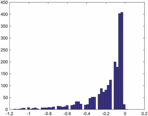
Figures 8 and 9 show the amount of soil temperature in each experiment and the soil temperature histogram.

Figure 8. The amount of soil temperature in each hour for 4 months.

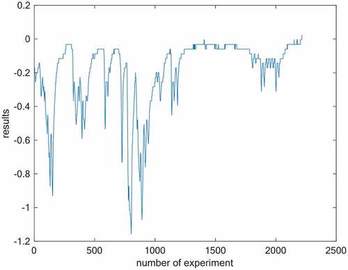
Figure 9. Soil temperature histogram.

Neural networks lead to an optimization problem after designing the structure for the training process. At first, we have used the gradient-based method of the neural network itself to train the weights of the neural network. But in a different approach, we have used Particle Swarm Optimization (PSO) and Genetic Algorithm (GA) methods for the training section of the weights of the neural network. The purpose of doing so was to compare the training methods for the weights of the neural network in this problem.

Predicting Soil Temperature Using MLP

The results of MSE and RMSE errors for training and test data for the MLP method are reported in Table 2.

Table 2. The results for errors in MLP method

Model	ANN
$MS{E}_{tr}$	0.0068
$MS{E}_{ts}$	0.0073
$RMS{E}_{tr}$	0.082
$RMS{E}_{ts}$	0.085

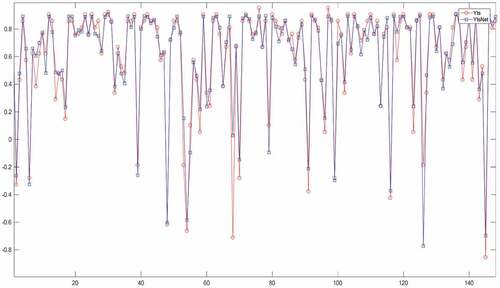
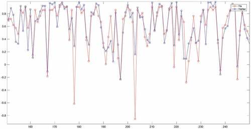
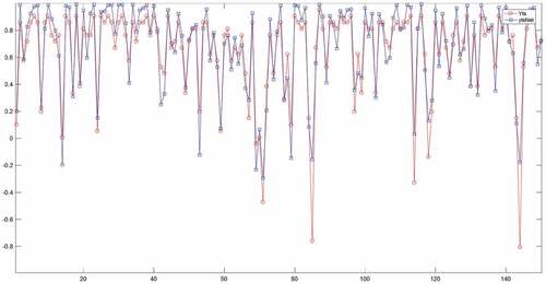
MSE_tr and MSE_ts show the mean square error for training and test data respectively and also RMSE_tr and RMSE_ts show the root mean square error of the training and test data. Figure 10 shows the comparison between training data and the output of the neural network for training data and Figure 11 displays shows the comparison between test data and the output of the neural network for test data.

Figure 10. Output error and the output of the network for training data.

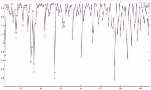
Figure 11. Output error and the output of the network for test data.

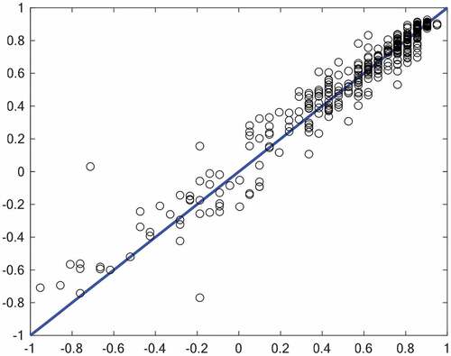
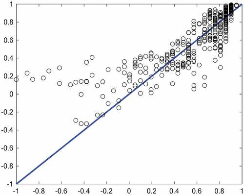
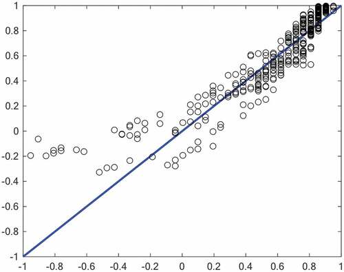
The regression plots for training and test data in the MLP method are shown in Figures 12 and 13.

Figure 12. Regression plot of the training data in the MLP method.

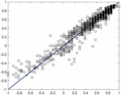
Figure 13. Regression plot of the test data in the MLP method.

Predicting Soil Temperature Using NN-GA

In this section, we have used the genetic algorithm optimization method for training the weights of the neural network. The results for the MSE and RMSE errors of the training and test data in the Neural Network-Genetic Algorithm (NN-GA) method are shown in Table 3.

Table 3. The results for errors in NN-GA method

Model	ANN
$MS{E}_{tr}$	0.038
$MS{E}_{ts}$	0.041
$RMS{E}_{tr}$	0.19
$RMS{E}_{ts}$	0.2

Figure 14 shows the comparison between training data and the output of the neural network for training data in the NN-GA method and Figure 15 displays shows the comparison between test data and the output of the neural network for test data in NN-GA method.

Figure 14. Output error and the output of the network for training data in NN-GA method.

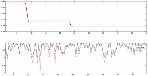
Figure 15. Output error and the output of the network for test data in NN-GA method.

The regression plots for training and test data in the NN-GA method are shown in Figures 16 and 17.

Figure 16. Regression plot of the training data in NN-GA method.

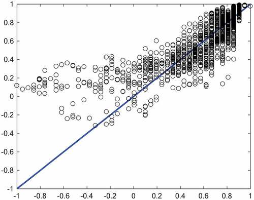
Figure 17. Regression plot of the test data in NN-GA method.

Predicting Soil Temperature Using NN-PSO

In this section, we have used the PSO algorithm optimization method for training the weights of the neural network. The results for the MSE and RMSE errors of the training and test data in the Neural Network- Particle Swarm Optimization (NN-PSO) method are shown in Table 4.

Table 4. The results for errors in NN-PSO method

Model	ANN
$MS{E}_{tr}$	0.018
$MS{E}_{ts}$	0.02
$RMS{E}_{tr}$	0.13
$RMS{E}_{ts}$	0.14

Figure 18 shows the comparison between training data and the output of the neural network for training data in the NN-PSO method and Figure 19 displays shows the comparison between test data and the output of the neural network for test data in NN-PSO method.

Figure 18. Output error and the output of the network for training data in NN-PSO method.

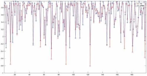
Figure 19. Output error and the output of the network for test data in NN-PSO method.

The regression plots for training and test data in the NN-PSO method are shown in Figures 20 and 21.

Figure 20. Regression plot of the training data in NN-PSO method.

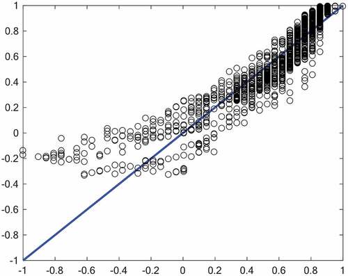
Figure 21. Regression plot of the test data in NN-PSO method.

As observed, according to the obtained values for root mean square error and mean error of the training and test data, training the neural network with the neural network gradient-based algorithm is done quite successfully. Therefore, among three MLP, NN-GA, and NN-PSO methods that we implemented, we propose MLP method as the superior method for predicting soil temperature from air temperature, relative humidity, and soil water content characteristics. The results for statistical hypothesis tests for soil temperature are reported in Table 5.

Table 5. The results for statistical hypothesis tests

Test	Value
P-Value	< 2.2e-16
T-Value	−44.044
df	2214
CI	[−0.2060935 − 0.1885232] ]
Mean	−0.1973084

As T-Value increases toward the positive or negative values, a higher possibility will exist for rejecting the null-hypothesis. The values of T-Value and P-Value are related in an inseparable way. Higher absolute values of T-Value will lead to lower Values for P-Value which decreases the probability of accepting the null-hypothesis and increasing its rejection.

Discussion

Frostbite is one of the biggest problems in the agricultural industry. Controlling and predicting daily soil temperature during winter is paramount for estimating frostbite. Some current methods predict the temperature of soil based on energy balance and soil heat flow. But these methods need a large amount of meteorological data, which is sometimes hard to obtain or unavailable. For example in (Kang et al. 2000), a hybrid soil temperature model was presented to estimate daily spatial and temporal patterns of soil temperature. This model was designed based upon heat transfer physics and the empirical relationship between air temperature and soil temperature. The data used in this study was obtained from satellite imagery, digital elevation, and standard weather records. Another study (Feng et al. 2019) was proposed four types of machine learning techniques to predict soil temperature as follows; the generalized regression neural networks (GRNN), extreme learning machine (ELM), random forests (RF), and backpropagation neural networks (BPNN). Based on these methods, half-hourly soil temperature was modeled at four different depths of 2 cm, 5 cm, 10 cm, and 20 cm. Meteorological data used for this study are solar radiation, vapor pressure, wind speed, relative humidity, and air temperature. Soil temperature is affected by several important properties such as air temperature, soil water content, topography, etc. Nevertheless, researchers in (Araghi et al. 2017) used only surface air temperatures to predict soil temperatures. In this study, the estimated soil temperature at 0300, 0900, and 1500 GMT utilizing artificial neural network (ANN) and wavelet transform artificial neural network (WANN) models. In (Ozturk, Salman, and Koc 2011) used geographical and meteorological data used to estimate soil temperature at 5-, 10-, 20-, 50-, and 100-cm depths. These variables are altitude, latitude, longitude, month, year, monthly solar radiation, monthly sunshine duration, and monthly mean air temperature. In this study, first of all, we focused on the relationship between soil temperature and other environmental variables. Our main goal was to predict soil temperature based upon minimum input variables without loss of prediction accuracy. For this reason, air temperature, soil water content, and relative humidity were selected for the training phase to estimate soil temperature. Next step, we were focused on the data set that was needed for estimating soil temperature. Precise temperature predictions of soil temperature need precise environmental data. For this purpose, environmental parameters can be acquired by environmental sensors. In most prior research, the soil temperature is estimated monthly, while daily or hourly recorded soil temperatures are more helpful for agricultural goals because of affecting chemical and biological processes. In contrast to many theoretical researches, the dataset used in this study is acquired by a HOBO U30 data logger. This device has an internal memory for storing environmental data such as soil humidity, soil temperature, air temperature, and relative humidity and also has sensors to measure these features. Environmental information is gathered hourly using these sensors. Finally, a predictive model was designed for soil temperature. Machine learning models are commonly used for estimation application. Artificial Neural Network (ANN) is one type of machine learning that has been used for designing prediction systems because of learning and modeling non-linear and complicated relationships. Decision Tree, Random Forest (RF), and XGBoost are other machine learning models. These models are tree-based and, for this reason, not very strong in extrapolating target values beyond training data limits. This is an important limitation for regression goals. In this study ANN had been successfully implemented for modeling soil temperature prediction from environmental data. Figure (9) shows the distribution of soil temperature. The regression lines depict the relationship between the actual output and network output in the graph. Figures 12, 16, and 20, the X-axis (horizontal axis) represents the Ytr while the Y-axis (vertical axis) represents the YtrNET in the MLP, NN-GA, and NN-PSO method, respectively. Similarly, Figures 13, 17, and 21 the X-axis (horizontal axis) represents the Yts and the Y-axis (vertical axis) represents the YtsNET in the MLP, NN-GA, and NN-PSO method, respectively. Regression plots show that MLP has better performance than ANN-GA and ANN-PSO networks. According to obtained results, MLP has high accuracy due to the lowest RMSE and MSE in both training and testing phase, compared to ANN-GA and ANN-PSO networks to prediction of soil temperature. The results for statistical hypothesis tests for soil temperature are reported in Table 5. In this research, we use a significance level of 0.05. As can be seen, the P-value is less than 0.05. Therefore, we can reject the null hypothesis. Rejecting the null hypothesis means that our findings were statistically significant. Farmers, botanical researchers, and policymakers in food security can use these results

Conclusion

In this paper, soil temperature was predicted based on air temperature, soil water content, and relative humidity using MLP neural network and compared with GA-ANN and PSO-ANN modals. Like any research project, data gathering is necessary, and numerous aspects play a role in this process. Nevertheless, three aspects have a more critical role that includes: the cost of the chosen data gathering approach, the accuracy and the performance of the data set. Neural networks, similar to many machine learning methods, are data-eating algorithms and need a large number of training data to provide actual and acceptable results. The above are the limitations of this study and any similar research that should be considered. Unlike many theoretical studies about soil temperature, this study was based on data provided by the HOBO U30 data logger device. This device is equipped with environmental sensors and gathers information hourly. The data used in this research is provided by the University of Toronto in Canada. The result showed that using the MLP model due to smaller MSE and RMSE had high accuracy and better predictive performance than ANN-GA and ANN-PSO models. Consequently, MLP was selected to predict soil temperature on cold days to prevent frostbite damage in crops.

Disclosure statement

No potential conflict of interest was reported by the author(s).

Additional information

Funding

This work was supported by the Babol Noshirvani University of Technology [BNUT/1399/393049].

References

- Araghi, A., M. Mousavi‐Baygi, J. Adamowski, C. Martinez, and M. van der Ploeg. 2017. Forecasting soil temperature based on surface air temperature using a wavelet artificial neural network. Meteorological Applications 24 (4):603–611. doi:10.1002/met.1661.
- Ardabili, S., A. Mosavi, A. Mahmoudi, T. M. Gundoshmian, S. Nosratabadi, and A. R. Várkonyi-Kóczy (2019, September). Modelling temperature variation of mushroom growing hall using artificial neural networks. In International Conference on Global Research and Education (pp. 33–1719). Springer, Cham. 10.1007/978-3-030-36841-8_3
- Atkinson, B. W. 2003. The climate near the ground, R. Geiger, RH Aron and P. Todhunter, xviii+ 584. Lanham, MD, USA: Rowman and Littlefield Publishers. doi:10.1002/joc.967.
- Barlow, K. M., B. P. Christy, G. J. O’leary, P. A. Riffkin, and J. G. Nuttall. 2015. Simulating the impact of extreme heat and frost events on wheat crop production: A review. Field Crops Research 171:109–19.
- Cadenas, J. M., M. C. Garrido, R. Martínez-España, and M. A. Guillén-Navarro. 2020. Making decisions for frost prediction in agricultural crops in a soft computing framework. Computers and Electronics in Agriculture 175:105587. doi:10.1016/j.compag.2020.105587.
- Chatterjee, S., N. Dey, and S. Sen. 2018. Soil moisture quantity prediction using optimized neural supported model for sustainable agricultural applications. Sustainable Computing: Informatics and Systems. doi:10.1016/j.suscom.2018.09.002.
- Ding, L., K. Noborio, and K. Shibuya. 2019. Frost forecast using machine learning-from association to causality. Procedia Computer Science 159:1001–10. doi:10.1016/j.procs.2019.09.267.
- Fath, A. H., F. Madanifar, and M. Abbasi. 2020. Implementation of multilayer perceptron (MLP) and radial basis function (RBF) neural networks to predict solution gas-oil ratio of crude oil systems. Petroleum 6 (1):80–91. doi:10.1016/j.petlm.2018.12.002.
- Feng, Y., N. Cui, W. Hao, L. Gao, and D. Gong. 2019. Estimation of soil temperature from meteorological data using different machine learning models. Geoderma 338:67–77. doi:10.1016/j.geoderma.2018.11.044.
- Gobbett, D. L., U. Nidumolu, H. Jin, P. Hayman, and J. Gallant. 2021. Minimum temperature mapping augments Australian grain farmers’ knowledge of frost. Agricultural and Forest Meteorology 304-305:108422. doi:10.1016/j.agrformet.2021.108422.
- Heidari, M., and H. Shamsi. 2019. Analog programmable neuron and case study on VLSI implementation of Multi-Layer Perceptron (MLP). Microelectronics Journal 84:36–47. doi:10.1016/j.mejo.2018.12.007.
- Kang, S., S. Kim, S. Oh, and D. Lee. 2000. Predicting spatial and temporal patterns of soil temperature based on topography, surface cover and air temperature. Forest Ecology and Management 136 (1–3):173–184. doi:10.1016/S0378-1127(99)00290-X.
- Keshavarzi, A., F. Sarmadian, E. S. E. Omran, and M. Iqbal. 2015. A neural network model for estimating soil phosphorus using terrain analysis. The Egyptian Journal of Remote Sensing and Space Science 18 (2):127–35. doi:10.1016/j.ejrs.2015.06.004.
- Liakos, K. G., P. Busato, D. Moshou, S. Pearson, and D. Bochtis. 2018. Machine learning in agriculture: A review. Sensors 18 (8):2674. doi:10.3390/s18082674.
- Liu, Y., J. C. Zhu, and Y. Cao. 2017. Modeling effects of alloying elements and heat treatment parameters on mechanical properties of hot die steel with back-propagation artificial neural network. Journal of Iron and Steel Research International 24 (12):1254–60. doi:10.1016/S1006-706X(18)30025-6.
- Maren, A. J., C. T. Harston, and R. M. Pap. 2014. Handbook of neural computing applications. Elsevier Academic Press.
- Messikh, N., S. Bousba, and N. Bougdah. 2017. The use of a multilayer perceptron (MLP) for modelling the phenol removal by emulsion liquid membrane. Journal of Environmental Chemical Engineering 5 (4):3483–89. doi:10.1016/j.jece.2017.06.053.
- Mohammadi, H., M. Moghbel, and F. Ranjbar. 2016. Prediction of soil frost penetration depth in northwest of Iran using air freezing indices. Theoretical and Applied Climatology 126 (3–4):533–41. doi:10.1007/s00704-015-1564-1.
- Nilsen, E. T., and D. M. Orcutt. 1996. Physiology of plants under stress. Abiotic factors. Physiology of Plants under Stress. Abiotic Factors 72:4.
- Nosratabadi, S., K. Szell, B. Beszedes, F. Imre, S. Ardabili, and A. Mosavi. (2020, October). Comparative analysis of ANN-ICA and ANN-GWO for crop yield prediction. In 2020 RIVF International Conference on Computing and Communication Technologies (RIVF) (pp. 1–5). Ho Chi Minh City, Vietnam: IEEE. doi: 10.1109/RIVF48685.2020.9140786
- Nosratabadi, S., S. Ardabili, Z. Lakner, C. Mako, and A. Mosavi. 2021. Prediction of food production using machine learning algorithms of multilayer perceptron and ANFIS. Agriculture 11 (5):408. doi:10.3390/agriculture11050408.
- Ochsner, T. E., R. Horton, and T. Ren. 2001. A new perspective on soil thermal properties. Soil Science Society of America Journal 65 (6):1641–47. doi:10.2136/sssaj2001.1641.
- Ozturk, M., O. Salman, and M. Koc. 2011. Artificial neural network model for estimating the soil temperature. Canadian Journal of Soil Science 91 (4):551–562. doi:10.4141/cjss10073.
- Paul, K. I., P. J. Polglase, P. J. Smethurst, A. M. O’Connell, C. J. Carlyle, and P. K. Khanna. 2004. Soil temperature under forests: A simple model for predicting soil temperature under a range of forest types. Agricultural and Forest Meteorology 121 (3–4):167–182. doi:10.1016/j.agrformet.2003.08.030.
- Qaderi, K., V. Jalali, S. Etminan, M. M. Shahr-babak, and M. Homaee. 2018. Estimating soil hydraulic conductivity using different data-driven models of ANN, GMDH and GMDH-HS. Paddy and Water Environment 16 (4):823–33. doi:10.1007/s10333-018-0672-9.
- Steponkus, P. L., M. Uemura, and M. S. Webb. 1993. Redesigning crops for increased tolerance to freezing stress. In Interacting stresses on plants in a changing climate, ed. Colin R. Black and Michael B. Jackson, 697–714. Berlin, Heidelberg: Springer. doi:10.1007/978-3-642-78533-7_45.
- Taheri, E., S. Tarighi, and P. Taheri. 2014. Identification and population estimation of epiphytic ice nucleation active bacteria isolated from stone fruit trees in Khorasan-Razavi Province. Journal of Plant Protection 29 (3):449–58. doi:10.22067/jpp.v29i3.44334.
- Vahedi, A. A. 2017. Monitoring soil carbon pool in the Hyrcanian coastal plain forest of Iran: Artificial neural network application in comparison with developing traditional models. Catena 152:182–89. doi:10.1016/j.catena.2017.01.022.
- Varol, T., A. Canakci, and S. Ozsahin. 2015. Modeling of the Prediction of densification behavior of powder metallurgy Al–Cu–Mg/B 4 C composites using artificial neural networks. Acta Metallurgica Sinica (English Letters) 28 (2):182–95. doi:10.1007/s40195-014-0184-6.
- Were, K., D. T. Bui, Ø. B. Dick, and B. R. Singh. 2015. A comparative assessment of support vector regression, artificial neural networks, and random forests for predicting and mapping soil organic carbon stocks across an Afromontane landscape. Ecological Indicators 52:394–403. doi:10.1016/j.ecolind.2014.12.028.
- Wu, J., and D. L. Nofziger. 1999. Incorporating temperature effects on pesticide degradation into a management model. Journal of Environmental Quality 28 (1):92–100. doi:10.2134/jeq1999.00472425002800010010x.