A Reinforcement Learning Based Decision Support Tool for Epidemic Control: Validation Study for COVID-19

ABSTRACT

Epidemics such as COVID-19 present a substantial menace to public health and global economies. While the problem of epidemic forecasting has been thoroughly investigated in the literature, there is limited work studying the problem of optimal epidemic control. In the present paper, we introduce a novel epidemiological model (EM) that is inherently suitable for analyzing different control policies. We validated the potential of the developed EM in modeling the evolution of COVID-19 infections with a mean Pearson correlation of 0.609 CI 0.525–0.690 and P-value < 0.001. To automate the process of analyzing control policies and finding the optimal one, we adapted the developed EM to the reinforcement learning (RL) setting and ran several experiments. The results of this work show that the problem of optimal epidemic control can be significantly difficult for governments and policymakers, especially if faced with several constraints at once, hence, the need for such machine learning-based decision support tools. Moreover, it demonstrated the potential of deep RL in addressing such real-world problems.

Introduction

Epidemics present a substantial menace to public health and global economies. In one year, from December 2019 to December 2020, the number of COVID-19 infections and deaths around the world reached 80 million and 2 million, respectively (WHO 2020). The exceptional public health interventions that have been undertaken show the degree of threat epidemics can present to governments, public health, health-care systems as well as global economies (Ferguson et al. 2020; WHO 2020). Measures such as lockdown and travel restriction are essential given the high infection rate of COVID-19 and the limited resources of hospitals. These non-pharmaceutical measures become even more important when the epidemic is caused by a new virus and no medication or vaccine is available. However, implementing such measures in a naïve way for a long time can cause serious damage to other important sectors, such as the economy. Researchers have developed epidemiological models (EMs) such as the susceptible-infected-recovered (SIR) and susceptible-exposed-infected-recovered (SEIR) models, as well as their variants (Giordano et al. 2020; Ian, Mondal, and Antonopoulos 2020; Prague et al. 2020; Santos, Almeida, and de Moura 2021; Sun et al. 2020) to anticipate the evolution of the disease, and accordingly design public health policies. However, recent studies such as (Eker 2020; Moein et al. 2021) has shown that most EMs developed for forecasting the evolution of COVID-19 are inefficient, either because of their inability to model the dynamics of the disease in the case of simple EMs, their reliance on the availability of big datasets in the case of machine learning-based EMs, or their overcomplexity which makes the optimization of their parameters difficult in the case of larger EMs. Only a few EMs showed significant efficiency, among these is the SIDARTHE model by (Giordano et al. 2020). SIDARTHE stands for susceptible (S), infected (I), diagnosed (D), ailing (A), recognized (R), threatened (T), healed (H), and extinct (E) cases. Because the SIDARTHE model was able to fit the real data accurately, it was used to inform global public health policies. However, since in most cases policies are manually designed, their optimality cannot be guaranteed. Moreover, most policies are designed without consideration for other important constraints besides mitigating the damage to public health.

While the epidemic forecasting problem is thoroughly investigated in the literature. The problem of optimal epidemic control is limitedly addressed. In this respect, approaches such as age-based lockdown (Daron et al. 2020) and n-work-m-lockdown (Karin et al. 2020) were proposed. However, due to the large space of possible policies (each with certain intensity), the number of dependent variables (behavioral, epidemic, demographic, etc.), the non-trivial trade-off impact both on public health and on the economy, the task becomes very demanding in terms of computational performance and efficiency especially because these traditional methods require the exploration of all possible options to ensure optimality.

In the last decade, an emerging field of the area of machine learning has demonstrated tremendous success in decision-making problems, that is, Reinforcement learning (RL). RL (Richard, Sutton, and Barto Andrew 2017) is a subclass of machine learning that deals mainly with learning optimal sequential decision-making. In RL, an agent is trained by interacting with an environment to maximize a reward. The success of RL is due to three main distinguishing reasons: firstly, the RL agent inherently accounts for, not only immediate costs/rewards but also, for future ones, resulting in learning the optimal sequence of actions for the tested environment (instead of each action independently). Secondly, RL is not bounded by human supervision data as in supervised learning, therefore, the performance of an RL agent might exceed human levels as demonstrated in many occasions such as (Mnih et al. 2013). Finally, RL combined with deep learning (i.e., Deep RL) can handle problems presented with large spaces, such as the game Go (Silver et al. 2017), which was considered an impossible task given the theoretical complexity of more than 10¹⁴⁰ possible solutions (Herik, H. Jaap, Jos, and Van Rijswijck 2002).

Regarding the use of RL for epidemic control, recent investigations were elaborated. For instance, in (Probert et al. 2019), RL was investigated for foot-and-mouth disease control, and similarly for the influenza pandemic (Libin et al. 2021). Recently, for the ongoing pandemic of COVID-19, RL-based approaches were proposed for optimal control and containment of the spread of the disease (Arango and Pelov 2020; Harshad, Ganu, and Seetharam 2020; Ohi et al. 2020; Padmanabhan et al. 2021). However, in the explored literature, the provided EMs-based environments are either restricted to a specific disease other than COVID-19 as in (Libin et al. 2021; Probert et al. 2019) or allow limited policy space, such as cyclic lockdown only, or on/off control as in (Arango and Pelov 2020; Harshad, Ganu, and Seetharam 2020; Ohi et al. 2020; Padmanabhan et al. 2021).

In the present paper, we investigate an RL-based approach for automating the process of analyzing and recommending control policies given different constraints in the context of epidemics. At first, we wanted to use an existing EM to adapt it to the RL setting and use it as an environment for training RL agents. For this, the SIDARTHE model discussed previously seemed a better candidate. However, as mentioned by the authors of the model, finding a solution for SIDARTHE is computationally complex. It is worth mentioning that the computational complexity of the SIDARTHE model was addressed in recent work by (Khalilpourazari and Hashemi Doulabi 2021b, 2021a; Khalilpourazari et al. 2021; Khalilpourazari, Soheyl, and Hossein Hashemi 2021). Indeed, in (Khalilpourazari and Hashemi Doulabi 2021b), the authors proposed a stochastic fractal search algorithm that can find a high-quality solution for the SIDARTHE model and efficiently determines many epidemiological parameters, thus, solving the EM in a relatively short time with high accuracy. In (Khalilpourazari et al. 2021), they introduced another approach for the same purpose as previously, accelerating the convergence of the search for optimal solutions for the SIDARTHE model. The proposed algorithm was named Gradient-based Grey Wolf Optimizer (GGWO), which according to the authors, it has demonstrated superior performance to most existing algorithms. In (Khalilpourazari and Hashemi Doulabi 2021a; Khalilpourazari, Soheyl, and Hossein Hashemi 2021), the authors designed a hybrid reinforcement learning (RL) based algorithm to efficiently solve the SIDARTHE model. The algorithm uses Q-learning (Richard, Sutton, and Barto Andrew 2017) to learn to switch between six optimization algorithms to maximize a defined reward that is proportional to the quality of the resulting solution.

Although the computational complexity of the SIDARTHE model was mitigated in the explored work, incorporating public health interventions in the dynamics of the model for policy optimization as well will most likely increase the complexity anew, especially when adding more constraints to the policy optimization process, which might diverge us from the focus of this paper. For this reason, in the present paper, we aim to develop a novel EM designed specifically for this task (i.e., RL-based analysis and recommendation of epidemic control policies). Despite being specifically developed for policy optimization; the developed EM must demonstrate at least acceptable efficiency in modeling the evolution of the disease as well to be of practical use. Therefore, we will validate the developed EM using real data of the evolution of COVID-19 in 10 Moroccan cities before using it for policy optimization.

The remainder of this paper is set as follows: In section 2, we present the EM we developed, its mathematical dynamics, and its validation result. In section 3, we adapt the developed EM to the RL setting, test the performance of selected deep RL algorithms, and conduct experiments inspired by real scenarios of epidemic control. Finally, in section 4, we summarize and discuss the main contributions of this research and provide future directions.

The Epidemiological Model

Dynamics of the Epidemiological Model

We aim to develop an EM that incorporates the impact of most public health measures in its dynamics to be inherently suitable for optimal control policies analysis and recommendation. To base our EM on solid theoretical foundations, we exploited the results of several state-of-the-art studies from the literature of epidemiology that can be summarized into the following points:

The reproduction rate (R0) of COVID-19 varies between a value of 1.4 and 2.4. additionally, demographic density and population size contribute proportionally to the increase of the infection rate of COVID-19 (Achaiah, Subbarajasetty, and Shetty 2020; Bhadra, Mukherjee, and Sarkar 2021; Kadi and Khelfaoui 2020).

Travel restriction, lockdown, social distancing, mask-wearing, and vaccination can considerably decrease the infection rate as explained in (Bergwerk et al. 2021; Chinazzi et al. 2020; Jarvis et al. 2020; Leech et al. 2021; Murano et al. 2021; Oraby et al. 2021).

High testing rate and isolation have an important role in lowering the number of infections per day as it helps identify asymptomatic carriers (Cohen and Leshem 2021; Mercer and Salit 2021).

An increase in the healthcare capacity (especially in intensive care units) can moderately help to reduce the mortality rate (Deschepper et al. 2021; Sen-Crowe et al. 2021).

Besides the healthcare capacity, the rate of fatality as well affects the mortality rate. The rate of fatality is inherent to the disease and varies from one to another (e.g., the fatality rate varies between 0.3% and 4.3% (Rajgor et al. 2020) for Coronavirus and around 85% for Ebola (Kadanali and Karagoz 2016)).

The probability of reinfection is around 16% only because the previous infection induces an effective immunity to future infections in most individuals (Hall et al. 2021; Okhuese 2020).

Studies such as (Bergwerk et al. 2021) suggest that vaccinated individuals may still get infected. The rate of effectiveness of the vaccine discussed in the mentioned study is around 61%. That is, only 61% of vaccinated individuals are guaranteed to have effective immunity against COVID-19.

Given the points above, and the RL setting. In the following, we define actions (A1-A7) that represent public health interventions, and states (S1-S4) describing current measurements of the evolution of the epidemic as well as the mathematical relationships between them:

• A1: Travel restriction

• A2: Lockdown

• A3: Distance work and education

• A4: Provide masks and impose their wearing

• A5: Increase the testing rate (test and isolate if positive)

• A6: Increase the health-care capacity (e.g., hospital beds)

• A7: Increase the vaccination rate

• S1: The transmission rate

• S2: The identification rate

• S3: The death rate

• S4: The probability of reinfection

The transmission rate (s1) represents the proportion of individuals that will be infected among a normal population. Formulated as:

(1) $s1=\left\{\begin{array}{c}\left[\left(1-\frac{A1+A2+A3+A4}{4}\right)\ast Density\ast \left(R0+\frac{CurInf}{N}\right)\right]-\left(A7\ast 0.61\right),ifV=1\\ \left[\left(1-\frac{A1+A2+A3+A4}{4}\right)\ast Density\ast R0\ast \frac{CurInf}{N}\right],ifV=0\end{array}\right.$(1)

where V is the availability of vaccines. That is, as explored previously (in points (1) and (2)), the transmission rate gets reduced if more travel restriction, lockdown, social distancing, mask-wearing were imposed. However, it is increased if the density of the studied region is high. The reproduction rate (R0) contributes proportionally to the transmission rate. Additionally, we consider that the more infections exist currently compared to the normal population, the higher the R0 should be. For this, we set the R0 to its minimum value (1.4) mentioned previously and add to it the value of the ratio $\frac{CurInf}{N}$, where N is the population size and Cur Inf is the number of current infections. This ratio will always be a small value given the huge values of N of regions (cities, countries, etc.) compared to the number of infected individuals. The last term in the equation is to model the impact of vaccination. Given point (7), if vaccination is implemented (V = 1), the transmission rate is reduced by 61% that represents the effectiveness of the vaccine investigated in the mentioned study.

Note that the value of the density is mapped from the real scale to a scale of values between 0 and 1. Please, see appendix A for more details.

The identification rate (s2): Here, we hypothesize that besides the role of the testing rate as explored in point (3), the incubation period and the severity of the symptoms also affect the identification of carriers. The longer the incubation period and the less severe are the symptoms, the less identifiable a disease becomes. COVID-19, for instance, has an incubation period that varies between 6.5 and 12.5 days (Quesada et al. 2021), often followed by moderate to no symptoms, as opposed to Ebola, for example, whose incubation period is around 12.7 days (Martin, Dowell, and Firese 2011) followed by the severe manifestation of symptoms. This is among the main reasons COVID-19 has spread much more than other epidemics (the lack of symptoms for a longer period). Therefore, the equation for S2 is:

(2) $\mathrm{s}2=A5\ast \left(1-incubationperiod\right)$(2)

Note that the value of the incubation period is mapped from the real scale to a scale of values between 0 and 1. Please, see appendix A for more details.

The death rate (s3): based on points (4) and (5), the death rate is proportional to the fatality rate inherent to the disease, and the more we invest in the healthcare capacity, the more we can mitigate the death rate. Thus, it is formalized as:

(3) $\mathrm{s}3=\left(1-A6\right)\ast fatalityrate$(3)

The reinfection rate (s4): based on points (6) and (7), the reinfection rate is formalized as the portion of individuals that are the non-effectively vaccinated times a probability of reinfection of around 16%:

(4) $\mathrm{s}4=\left(1-\left(A7\ast 0.61\right)\right)\ast Probabilityofreinfection$(4)

Population Class Model Based on the Elaborated Dynamics

To clarify even further, we developed a population-class model illustrated in Figure 1 that is driven by the above-explained epidemiological dynamics, where: Cur Inf: current infections, N: normal population, First Inf: individuals infected for the first time, Re Inf: individuals reinfected after recovery from a previous infection, Nxt Inf: next (predicted) infections, U: unknown carriers, K: known carriers, R: recovered, D: deaths, s1: the transmission rate, s2: the identification rate, s3: the death rate, s4: the reinfection rate.

Figure 1. Population class model for the developed EM.

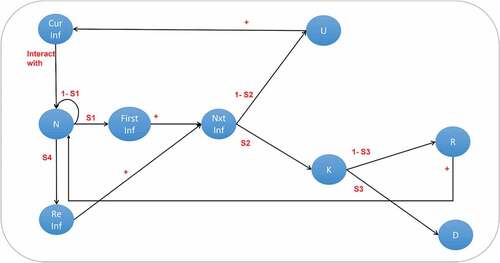
We consider that a region with a normal (i.e., not infected) population size “N,” will be in contact with an initial number of current infected individuals “Cur Inf” (e.g., came from another infected region) and will generate an s1*N number of new primary infections “First Inf” (i.e., with no COVID-19 history), and s4*R reinfected individuals, where R represents the number of recovered individuals. Both primary infected and reinfected will be added to the next infected “Nxt Inf” class where they will be divided into two other classes, either known carriers “K” or unknown carriers “U” depending on the identification rate s2. The unknown carriers “U” (e.g., those that did not show symptoms nor have been tested) will be added to the current infections “Cur Inf” for the next iteration since they contribute to the number of infections because they are not aware of their infection. The known carriers (e.g., those that were tested positive and hospitalized) will either die according to the death rate s3 and get subtracted from the global population “N” or recover and get added to the global population.

In equations (5(5) $\mathrm{C}\mathrm{u}\mathrm{r}\mathrm{I}\mathrm{n}\mathrm{f}=CurInf+U$(5) –13(13) $\mathrm{D}=s3\ast K$(13) ) and Table 1, we present a summary of all variables and parameters used in the developed EM.

(5) $\mathrm{C}\mathrm{u}\mathrm{r}\mathrm{I}\mathrm{n}\mathrm{f}=CurInf+U$(5)

(6) $\mathrm{N}=N-D$(6)

(7) $\mathrm{F}\mathrm{i}\mathrm{r}\mathrm{s}\mathrm{t}\mathrm{I}\mathrm{n}\mathrm{f}=s1\ast N$(7)

(8) $\mathrm{R}\mathrm{I}=s4\ast R$(8)

(9) $\mathrm{N}\mathrm{x}\mathrm{t}\mathrm{I}\mathrm{n}\mathrm{f}=FirstInf+ReInf$(9)

(10) $\mathrm{K}=s2\ast NxtInf$(10)

(11) $\mathrm{U}=\left(1-s2\right)\ast NxtInf$(11)

(12) $\mathrm{R}=\left(1-s3\right)\ast K$(12)

(13) $\mathrm{D}=s3\ast K$(13)

Table 1. Summary of the variables and parameters of the developed EM

Variables	Description
Cur Inf	Current infections in the studied region, initialized by the user at the first step, then changed automatically according to the dynamics of the simulation.
N	The population size of the studied region, initialized by the user at the first step, then changed automatically according to the dynamics of the simulation.
First Inf	The number of infected individuals for the first time, computed during the simulation.
Re Inf	The number of infected individuals after recovery (for the second time), computed during the simulation.
Nxt Inf	The number of next infection cases, (which is the sum of First Inf and Re Inf), computed during the simulation.
K	The number of known carriers, (those that were tested positive and hospitalized), computed during the simulation.
U	The number of unknown carriers, (those that neither showed symptoms nor have been tested), computed during the simulation.
R	The number of recovered cases, computed during the simulation.
D	The number of death cases, computed during the simulation.
Parameters	Description
R0	The reproduction rate of the studied epidemic. Varies between 1.4 and 2.4.
Incubation	The incubation period of the studied epidemic. Varies between 5.6 and 12.5 days.
Fatality	The fatality rate of the studied epidemic when no healthcare treatment is taken. Varies between 0.3% and 4.3%.
Reinfection	The reinfection probability of the studied epidemic, fixed at 0.16.
Density	The density of the studied region (in people/km^2), defined by the user.
S1	The transmission rate, defined in equation (1)(1) $s1=\left\{\begin{array}{c}\left[\left(1-\frac{A1+A2+A3+A4}{4}\right)\ast Density\ast \left(R0+\frac{CurInf}{N}\right)\right]-\left(A7\ast 0.61\right),ifV=1\\ \left[\left(1-\frac{A1+A2+A3+A4}{4}\right)\ast Density\ast R0\ast \frac{CurInf}{N}\right],ifV=0\end{array}\right.$(1) .
S2	The identification rate, defined in equation (2)(2) $\mathrm{s}2=A5\ast \left(1-incubationperiod\right)$(2) .
S3	The death rate, defined in equation (3)(3) $\mathrm{s}3=\left(1-A6\right)\ast fatalityrate$(3) .
S4	The reinfection rate, defined in equation (4)(4) $\mathrm{s}4=\left(1-\left(A7\ast 0.61\right)\right)\ast Probabilityofreinfection$(4) .

Validation of the Developed EM

Although the developed EM is designed for policy optimization, it cannot be of practical use unless it demonstrates at least an acceptable efficiency in terms of modeling the evolution of the disease using real data. For this, we measured the Pearson correlation between the real epidemic evolution and the one given by the developed EM for 10 Moroccan cities. The needed data was as follows:

• The density and population size of the studied regions, available on the official website of the high planning commission of Morocco (HCP 2021).

• The real number of infected and dead individuals per day is available on the official website of the Ministry of Health of Morocco (Moroccan Minstry of Health 2020).

• The implemented public health interventions by the Moroccan government during each period. For this information, we exploited the results of studies such as (Masbah and Aourraz 2020; OECD 2020; PERC 2021a, 2021b) that tracked the public health interventions in Morocco as well as citizens’ respect for the implemented measures. Given that the reported results were relatively dissimilar, we decided to generate random values between 0 and 1 sampled from a uniform distribution to estimate the numerical values of each public health intervention in the following methodology:

  • For periods where the government imposed highly strict measures, a random number between 75% and 100% is generated for this measure for each day of that period.

  • For periods where the government imposed moderately strict measures, a random number between 50% and 75% is generated for this measure for each day of that period.

  • For periods where the government imposed leniently strict measures, a random number between 20% and 50% is generated for this measure for each day of that period.

  • For periods where the government imposed no measure, a random number between 0% and 20% is generated for this measure for each day of that period.

In appendix A, we provide more details about this step.

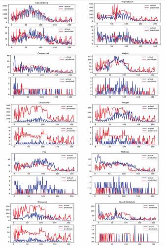
We gathered all the necessary data for a period of seven months, from September 3rd, 2020, to March 31st, 2021. In Figure 2, we present the results of evaluating the developed EM in modeling the course of COVID-19 in 10 Moroccan cities. As listed in Table 2, the mean Pearson correlation between the actual number of infections and the predicted ones is 0.609 CI 0.525–0.690 and P< .001. However, concerning the prediction of the number of deaths per day, the mean value of the correlation was 0.272 CI 0.201–0.342 with a mean P-value of P = .073 CI 0.010–0.13, opening the door for more improvement in this regard. Another observation is regarding the efficiency of the model according to the density of the studied region, the developed EM was most efficient for cities with a higher density such as Casablanca and Marrakech than cities with a lower density such as Ouad-Eddahab and Laayoune. This was a rather expected result because the authorities divided Moroccan cities into two zones, low-risk zones and high-risk zones (PERC 2021a), and implemented more strict measures and testing in high-risk zones. Given those dense regions such as Casablanca and Marrakech presented the biggest numbers of infections, therefore classified as high-risk zones, a high testing rate was conducted in those cities which strengthened the accuracy of the model. Whereas for regions with low testing rates, most of which have low density, the model showed an over-estimation of the infection rate.

Table 2. Summary of the result of the validation according to the population size and density for the 10 Moroccan cities

City	Population size	Density ppl/km2	Corr Inf/day	P-value Inf/day	Corr Death/day	P-value Death/day
Casablanca	3,535,127	11,380	0.758	1.68e-40	0.462	1.51e-12
Marrakech	1,393,206	6521	0.708	4.54e-32	0.422	1.63e-10
Ouarzazat	297,502	24	0.540	1.17e-10	0.203	0.072
Rabat	544,422	4853	0.750	2.43e-39	0.205	0.002
Tetouane	550,374	216.6	0.609	8.66e-23	0.261	0.001
O.Eddahab	126,765	1.82	0.372	6.34e-05	0.244	0.040
Fes	1,232,798	657.3	0.578	3.80e-20	0.175	0.190
Meknes	891,155	457.3	0.555	2.13e-18	0.220	0.201
Laayoune	256,482	5.3	0.559	1.08e-18	0.207	0.195
Tanger	1,188,815	7026	0.651	3.66e-14	0.324	0.033

Figure 2. The actual number of infections versus the predicted number of infections per day on top of each subfigure. The actual number of deaths versus the predicted number of deaths per day on the bottom of each subfigure, in the ten Moroccan cities.

Note that, in this experiment, we set V to 0 in equation (1)(1) $s1=\left\{\begin{array}{c}\left[\left(1-\frac{A1+A2+A3+A4}{4}\right)\ast Density\ast \left(R0+\frac{CurInf}{N}\right)\right]-\left(A7\ast 0.61\right),ifV=1\\ \left[\left(1-\frac{A1+A2+A3+A4}{4}\right)\ast Density\ast R0\ast \frac{CurInf}{N}\right],ifV=0\end{array}\right.$(1) since vaccines were not available at this time.

Deep RL for Epidemic Control

Adapting the Developed EM to the RL Setting

Besides the actions (A1-A7) and states (S1-S4) described in the previous section, in RL, a reward signal is defined to measure the performance of the agent. In our setting, we consider defining a sequence of actions that minimizes the infection rate with minimum investment in the seven actions to preserve the economy as the optimal policy the agent should seek. For this, we define the reward function as:

(14) $reward=\left\{\begin{array}{c}healthscore+economicscore,ifhealthscoreandeconomicscore>0\\ 0,otherwise\end{array}\right.$(14)

Where

(15) $healthscore=\left\{\begin{array}{c}\left(TI-NewInf\right)/TI,ifNewInf<TIandD<TD\\ 0,otherwise\end{array}\right.$(15)

TI and TD are thresholds for the infections (Nxt Inf) and the deaths (D) not to surpass.

(16) $\mathrm{e}\mathrm{c}\mathrm{o}\mathrm{n}\mathrm{o}\mathrm{m}\mathrm{i}\mathrm{c}\mathrm{s}\mathrm{c}\mathrm{o}\mathrm{r}\mathrm{e}=1-\frac{\sum \mathrm{w}\mathrm{i}\ast \mathrm{A}\mathrm{i}}{\sum \mathrm{w}\mathrm{i}}$(16)

On the one hand, the health score reflects the agent’s performance with respect to public health: the lesser is the number of infections compared to the set threshold TI, the higher will be the term “$\left(TI-NewInf\right)/TI$”. On the other hand, the economic score reflects obstacles (mainly budgetary) for investing too much in these actions for the sake of reducing the public health damage. As confirmed in (Jasper, Koks, and Hall 2021), measures such as long lockdown have serious consequences on the global economy. The weights w1-w7 applied on actions (A1-A7) in the economic score are used to enforce some preferred priorities in guiding the agent’s learning. That is, if in the studied region, the impact of a certain intervention is higher than other interventions, its weight should be much higher, this way, small changes in the action with high weight will induce greater impact. Furthermore, the two defined scores are inversely proportional, that is, to increase the economic score, the agent should not (or should rarely) apply actions, however, to increase the health score, the agent should apply high intensities of public health interventions (actions) to reduce the number of infections.

Implementing a Deep RL Agent for Policy Optimization

The environment based on the developed EM belongs to the category of continuous environments, meaning that, the state and action spaces are continuous, as opposed to discrete. Therefore, the agent that would be trained in this environment should support continuous control.

In RL, Q-learning is considered one of the basic, yet classic algorithms as it was founded in 1989. Q-learning learns by updating a Q-table that stores the values of each state-action pair using the Bellman equation (Richard, Sutton, and Barto Andrew 2017). The main drawback of Q-learning is its inability to (directly) learn in environments with continuous states and actions since it uses a Q-table that has a finite size. In 2013, deep Q-Network (DQN) by (Mnih et al. 2013) came up with a solution. DQN uses a function approximator (a neural network (NN)) instead of the Q-table to learn the Q-values for each state-action pair. The use of NN enabled supporting environments with continuous states because each state is mapped to its Q-value given via the NN which itself is a continuous function. Moreover, using NNs, the update rule became based on the gradient of the loss instead of the dynamic programming approach and the Bellman equation in Q-learning.

However, DQN is still faced with other challenges, mainly, handling environments with continuous actions as well (not continuous states only). Consequently, scientists have investigated other techniques. The main techniques used for continuous control nowadays are the policy gradient algorithms (Sutton et al. 1996). Policy gradient algorithms learn to directly map states to actions or a probability distribution over actions instead of their Q-values. Along with an architecture commonly known as the actor-critic (Konda and Tsitsiklis 2000) and deep neural networks as function approximators, where the actor (π) outputs actions and the critic (Q) evaluate these actions by assigning values to them, policy gradient emerged as a family of algorithms used in most state-of-the-art achievements, such as mastering the game of Go (Silver et al. 2017) and the game of StarCraft II (Sun et al. 2018).

Among the state-of-the-art models that use this approach is the deep deterministic policy gradient (DDPG) (Lillicrap et al. 2016). DDPG was designed to operate on potentially large continuous state and action spaces with a deterministic policy, meaning that the policy function (π) directly outputs an action as opposed to a stochastic policy, where the output is a probability distribution over actions. However, it is often reported that DDPG suffers from instability in the form of sensitivity to hyper-parameters and propensity to converge to very poor solutions or even diverge (Matheron, Perrin, and Sigaud 2019). For this, many algorithms were proposed as a solution for the problems faced by DDPG such as the twin delayed deep deterministic (TD3) policy gradient (Fujimoto, Van Hoof, and Meger 2018). TD3 solves the instability issue by (i) minimizing the overestimation bias through maintaining a pair of critics Q1 and Q2 (hence the name “twin”) along with a single actor. For each time step, TD3 uses the smaller of the two Q-values, and (ii) updates the policy less frequently than the critic networks. Another category of the policy gradient algorithms uses a stochastic policy, instead of a deterministic one. This makes the exploration phase automatically executed, in contrast to deterministic policy, where the exploration is handled manually. One of the main state-of-the-art models that uses this approach is the proximal policy optimization (PPO) (Schulman et al. 2017) algorithm. PPO involves collecting a mini batch of experiences while interacting with the environment and using it to update its policy. Once the policy is updated, a newer batch is collected with the newly updated policy, thus, it is an on-policy algorithm, as opposed to off-policy algorithms, where the function used to collect experiences is different from the one updated for learning. The key contribution of PPO is ensuring that a new update of the policy does not change it too much from the previous policy. This leads to less variance and smoother training and makes sure the agent does not go down an unrecoverable path.

Given the above introductory clarifications, in the following subsections, we run several experiments to validate the usefulness of deep RL in the context of epidemic control.

Experiment 1: DDPG, TD3, and PPO Performance

In this experiment, we tested and compared the performance of the three deep RL models discussed previously (DDPG, TD3, and PPO) to solve the environment given health score thresholds of different degrees of difficulty (TI and TD in equation (15)). We go from high thresholds (i.e., easy constraint) to low thresholds (i.e., difficult constraints). For the implementation phase, we used the DDPG described in the original paper (Lillicrap et al. 2016) but with the gaussian action noise instead of the Ornstein Uhlenbeck noise as it showed better performance (please see appendix B). The implemented TD3 is exactly the one described in the original paper (Fujimoto, Van Hoof, and Meger 2018). Finally, for PPO, we chose the clipped version instead of the Kullback–Leibler penalty implementation (Schulman et al. 2017). All three models have two hidden layers with 64 units each.

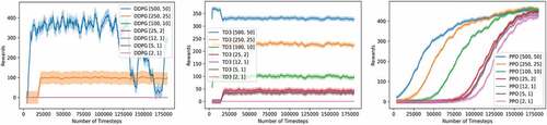
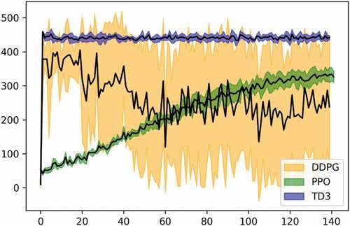
For the other hyperparameters, after testing and tuning, we used the ones yielding the best performance for each model, (please see Appendix B for more details on this step). As illustrated in Figure 3, the DDPG model suffered from a high variance for the first two easiest threshold sets, while yielding zero rewards for harder ones. TD3 on the other hand showed a better performance both in terms of the variance and the episodic reward. This was rather expected since TD3 came as a successor to DDPG, thus, solving its main theoretical issues. However, the best-performing model was PPO which showed excellent consistency even in the most difficult threshold set ([2, 1]) where TD3 failed. Moreover, PPO’s variance was around 4.8 which is close to TD3ʹs of around 3.6, but much better than DDPG’s of around 22.1. For PPO, the more the task is difficult, the more timesteps it needs to start converging to an optimal policy and yielding similar episodic reward as easier tasks, thus sacrificing only the training time, while DDPG and TD3 abdicate the episodic reward as well. Furthermore, it is worth mentioning that even so, PPO was still the fastest among the three in terms of the training speed with an important difference. Indeed, DDPG and TD3 lasted about 57 minutes for the 180,000steps of training, while PPO needed only a 6 min for the same number of steps on a CPU, i7, 10 generation, with IRIS plus accelerator. Given these comparison results, we excluded DDPG and TD3 for the remainder of the experiments and use PPO only.

Figure 3. Episodic reward and variance monitoring for the three models for different health score thresholds.

Experiment 2: PPO Performance against Different Economic Thresholds

In this part, we change in equation (14)(14) $reward=\left\{\begin{array}{c}healthscore+economicscore,ifhealthscoreandeconomicscore>0\\ 0,otherwise\end{array}\right.$(14) of the reward function to test more constrained versions of the task at hand, particularly, it will be changed to the following:

(17) $reward=\left\{\begin{array}{c}healthscore+economicscore,ifhealthscore>0andeconomicscore>Te\\ 0,otherwise\end{array}\right.$(17)

where Te is a threshold for the economic score. This means that the agent will not receive a positive reward unless the health score is positive (as previously) and the economic score is greater than the defined Te. This new reward function can be considered as a generalized version, wherein the previous reward function Te was always set to 0.

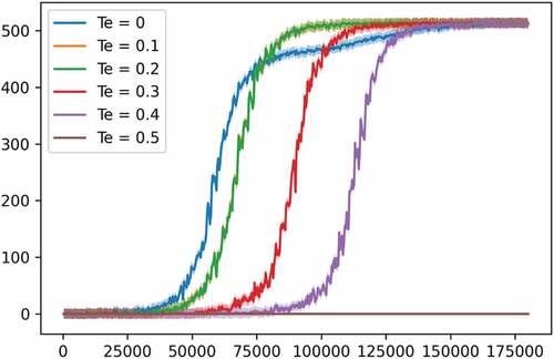
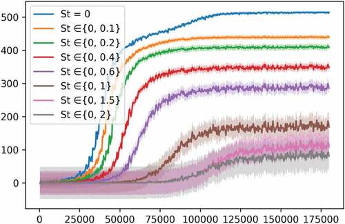
In Figure 4, we tested the capacity of the PPO model against different values for the economic score threshold Te and recorded its performance. The health score thresholds were set to 25 and 2 for TI and TD respectively. We can see that the higher is Te, the more steps are needed for the PPO model to start converging to a good policy. We kept increasing Te until a value of around 0.5, where the agent stopped getting any reward.

Figure 4. PPO performance against different economic thresholds (Te).

Experiment 3: PPO Policy Analysis regarding Custom Priorities

In experiment 1, we tested the deep RL models against different health score thresholds. In experiment 2, we constrained the reward function more by adding a threshold criterion on the economic score as well. In this experiment, the goal is to visualize the effect of having different priorities in guiding the agent’s policy: as explained earlier in equation (16)(16) $\mathrm{e}\mathrm{c}\mathrm{o}\mathrm{n}\mathrm{o}\mathrm{m}\mathrm{i}\mathrm{c}\mathrm{s}\mathrm{c}\mathrm{o}\mathrm{r}\mathrm{e}=1-\frac{\sum \mathrm{w}\mathrm{i}\ast \mathrm{A}\mathrm{i}}{\sum \mathrm{w}\mathrm{i}}$(16) of the economic score, the weights w1-w7 applied on actions (A1-A7) in the economic score are used to enforce some preferred priorities in guiding the agent’s learning. For instance, if the studied region relies heavily on the tourism sector, applying measures such as travel restriction and lockdown will have an important cost on the global economy of the region. Thus, the policymakers should define a control policy in an optimized way, investing more in low-cost measures within the context of that region without sacrificing the public health goals.

In Figure 5, we show the episodic reward (in the left subfigures) and the policy given by the agent for 12 months (in the right subfigures). We tested the effect of the weights used in the economic score on the performance of the agent using two sets of weights, one set has the same values and another set biased toward a preferred priority. In both experiments, the health score thresholds used are 25 for TI and 2 for TD, while Te is set to 0.

Figure 5. The effect of the economic score weights on the performance and policy.

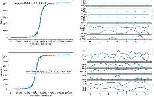
In the top two subfigures, the weights have the same values. The PPO model showed a good performance with a high episodic reward. Nevertheless, because the number of predicted infections “Nxt Inf” is related to the normal population (N) through the transmission rate (s1), where s1 includes only A1, A2, A3, and A4 (see equation (1)(1) $s1=\left\{\begin{array}{c}\left[\left(1-\frac{A1+A2+A3+A4}{4}\right)\ast Density\ast \left(R0+\frac{CurInf}{N}\right)\right]-\left(A7\ast 0.61\right),ifV=1\\ \left[\left(1-\frac{A1+A2+A3+A4}{4}\right)\ast Density\ast R0\ast \frac{CurInf}{N}\right],ifV=0\end{array}\right.$(1) ), the agent learned to reduce the infections by maximizing these four actions while keeping the other ones as low as possible. However, in the below subfigure, the weights are biased in such a way that investing in A1 and A2 will reduce the economic score greatly, thus reducing the reward. This way, the agent learned a more complex policy balancing the intensities of the applied actions. The agent learned that increasing the healthcare capacity reduces the number of deaths plus a relatively high vaccination rate compared to previous policy to reduce the reinfection rate that contributes to the infections as well. However, the performance (episodic reward) of the agent dropped from 500s to 350s, this again demonstrates the difficulty of the epidemic control problem, especially for hand designing optimal policies.

Note: the policy given by the agent is interpreted following the same guide used during the validation of the EM described in appendix A. That is because actions in our case are continuous, each one is quantized into four divisions: 0.75 to 1 for highly strict measures, 0.5 to 0.75 for moderately strict measures, 0.2 to 0.5 for leniently strict measures, and 0 to 0.2 for no measure. As an example, the first action, which is travel restriction, is interpreted as follows:

• 0.75–1: no travel is allowed between countries and cities.

• 0.5–0.75: only some types of travel (air travel, sea travel, within-country/within the city, etc.) are allowed with the condition to have permission papers, such as negative test for COVID-19.

• 0.2–0.5: most types of travel are allowed with the condition to have permission papers, such as negative test for COVID-19.

• 0–0.2: all travels are allowed.

For the interpretation of other actions, please refer to appendix A.

Experiment 4: Adding Stochasticity to the Environment

In the present experiment, we alter the equation of the transmission rate (s1) by adding a stochasticity parameter (St) that reduces the impact of actions (A1-A4) in a randomized way. The parameter St is randomly sampled from a uniform distribution between a defined range of {0, max St}, where max St is the maximum of this range. The new equation of s1 becomes:

(18) $s1=\left\{\begin{array}{c}\left[\left(1-\frac{A1+A2+A3+A4-St}{4}\right)\ast Density\ast \left(R0+\frac{CurInf}{N}\right)\right]-\left(A7\ast 0.61\right),ifV=1\\ \left[\left(1-\frac{A1+A2+A3+A4-St}{4}\right)\ast Density\ast R0\ast \frac{CurInf}{N}\right],ifV=0\end{array}\right.$(18)

This is useful because, in real scenarios, the same implemented measures by policymakers might have a different impact on the evolution of the disease because of the unpredictable rate of respect of these measures by citizens in each period or region.

In Figure 6, we show the result of training the PPO model when St is sampled from ranges of different sizes. We can see that when St varies in a bigger range, that is, the higher is the stochasticity of the environment, the more difficult it becomes for the agent to find an optimal policy, with higher variance displayed each time the size of the range is increased. This experiment demonstrates another aspect of the difficulties facing policymakers. The success of the implemented policies is proportional to the rate of respect for these policies by citizens. For instance, when St is sampled from the range {0, 0.2}, the agent learns a policy for a transmission rate that does not vary a lot, and the impact of its actions are not reduced significantly, meaning that only a minority of citizens did not respect the implemented measures. However, when St is sampled from a bigger range as {0, 2}, the agent’s actions will have a different impact each time. On some occasions, the sampled St is a relatively low (close to 0), meaning that the impact of the agent’s actions is not (or negligibly) reduced, while on other occasions, the sampled St is high (close to 2), meaning that the impact of the agent’s actions is significantly reduced, representing, a non-respect of the applied measures by a significant portion of citizens. Thus, encountering a successful state-action pair will have an uncertain degree of usefulness.

Figure 6. The effect of stochasticity on the performance of the PPO model.

Discussion

Main Contributions

Optimal epidemic control is a complex task for humans, and as demonstrated in the previous section, it can be difficult for state-of-the-art machine learning algorithms as well. The degree of difficulty is increased when more constraints must be fulfilled, and realistic aspects of the simulation dynamics are added. For this, having an EM that balances between efficiency and computational complexity is necessary.

In this paper, we introduced a novel EM that demonstrated a decent performance in modeling the course of COVID-19 to ensure the practicality of the results and conclusions deduced. The EM demonstrated a mean Pearson correlation of 0.609 CI 0.525–0.690 and P< .001. Despite being relatively simple, the developed EM was able to adapt to each region’s characteristics because it accounts for the impact of the implemented public health measures in those regions in addition to some demographic and epidemic characteristics. Once the EM was validated, we adapted it to the RL setting allowing it to be used not only for forecasting the evolution of the disease but also, training learning-based agents for policy optimization as well. Then, we ran several experiments where each one permitted us to deepen our insights into the problem at hand.

In experiment 1, we trained three state-of-the-art deep RL models (DDPG, TD3, and PPO) in the developed EM-based environment with eight different threshold sets of the health score (TI and TD) described in equation (15)(15) $healthscore=\left\{\begin{array}{c}\left(TI-NewInf\right)/TI,ifNewInf<TIandD<TD\\ 0,otherwise\end{array}\right.$(15) . Each threshold set increases the difficulty compared to the previous one. the PPO model showed a relatively good and consistent performance throughout all threshold sets, whereas DDPG, and besides its high variance, failed as soon as the third threshold set (100,10). TD3 on the other hand was better than DDPG, and its performance did not drop to zero until the last threshold set (2,1). Nevertheless, PPO outperformed TD3 in terms of the episodic reward in all threshold sets. For this, we excluded DDPG and TD3 and continued the rest of our experiments with PPO only. This experiment shows that stochastic policy-based models, such as PPO can be advantageous over deterministic policy-based models in this context.

In experiment 2, we modified the reward function to set custom thresholds on the economic score as well, named Te, adding more constraints to the agent’s policy. After fixing the health score thresholds to 25 and 2 for TI and TD, respectively, we kept changing Te from easy to more difficult allowing us to test the limits of our PPO model. In addition to experiment 1, this experiment as well demonstrates the difficulty facing policymakers in defining an optimal control policy, that is, the sequence of public health measures, each with a certain intensity, capable of optimizing the public health state while causing minimum harm to the economy while possessing limited budget represented here by Te. As a benchmarking result, our PPO model was successful in all tested thresholds until Te of 0.5 where it failed, and the performance dropped to zero.

Besides, this experiment emphasizes the importance of reward engineering. The reward functions described in equation (14)(14) $reward=\left\{\begin{array}{c}healthscore+economicscore,ifhealthscoreandeconomicscore>0\\ 0,otherwise\end{array}\right.$(14) or equation (17)(17) $reward=\left\{\begin{array}{c}healthscore+economicscore,ifhealthscore>0andeconomicscore>Te\\ 0,otherwise\end{array}\right.$(17) do not tell the agent much information. This was done on purpose to benefit from the model-free RL creativity because trivial reward functions often yield trivial policies, which in most cases are not helpful. In the following, we illustrate this statement by changing the reward function to a much easier one:

(19) $reward=\left\{\begin{array}{c}healthscore+economicscore,ifs1<Ts1\\ 0,otherwise\end{array}\right.$(19)

Where Ts1 is a threshold for s1 (the transmission rate).

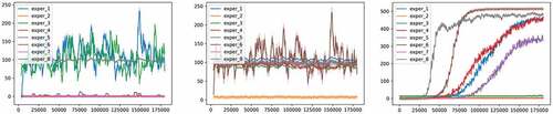
Here, the reward function is computed from the state s1, which is a direct input of the agent, thus, the exploration needed is reduced since the agent will learn to invest in measures that directly affect the state s1 only. Figure 7 shows that the needed number of training steps for the same deep RL models used previously is significantly reduced, and the performance is improved for DDPG and TD3 especially. However, having such a trivial reward function will yield a policy that is not flexible and may not be interesting or helpful for policymakers. Moreover, this way, even if s1 is set at a low value, it does not guarantee that the number of infections is minimized, this will depend on the population size: low value for s1 multiplied by a huge population size might still yield high values for the number of infections. Whereas in the previous reward functions, (i) the agent will encounter multiple choices that affect the reward function positively in different ways that may not be directly related to s1 yielding a flexible policy function and always guaranteeing that (ii) the number of infections is reduced.

Figure 7. The performance of the DDPG, TD3, and PPO on the easier reward function.

In experiment 3, we examined the output policy regarding another component in the reward function: the action weights in the economic score. This experiment justifies the use of the action weights in equation (16)(16) $\mathrm{e}\mathrm{c}\mathrm{o}\mathrm{n}\mathrm{o}\mathrm{m}\mathrm{i}\mathrm{c}\mathrm{s}\mathrm{c}\mathrm{o}\mathrm{r}\mathrm{e}=1-\frac{\sum \mathrm{w}\mathrm{i}\ast \mathrm{A}\mathrm{i}}{\sum \mathrm{w}\mathrm{i}}$(16) and especially demonstrates that the difficulty of defining optimal control policy is increased when some actions present higher costs than others.

Finally, in experiment 4, we presented another aspect of the difficulties facing policymakers, that is, the unpredictable rate of respect of measures by citizens that may reduce the impact of these implemented measures in variant degrees. This experiment opens the door for future improvements in the algorithm behind the agent to handle such realistic constraints.

Limitations and Future Directions

The actual chronology of disease outbreaks indicates that the frequency of occurrence is rising, especially in today’s world of rapid globalization, and that we are more liable to undergo many such pandemics in the near term (World Health Organization 2015). Consequently, reinforcing the collaborative efforts between epidemiologists, computer scientists, economists, etc. to help mitigate their damages is a necessity. In the present work, we introduce an aspect of reinforcing this collaboration by introducing a novel RL-based tool for epidemic modeling and control. The presented tool has shown the potential of usefulness in modeling the evolution of the number of COVID-19 infections per day, and in suggesting optimal control policies using a trained RL agent. However, further improvements from all epidemiology and optimization-related disciplines are still needed. In the following, we list the main limitations and future directions of the current version of the presented tool:

Although the developed EM showed a significant correlation in the tested 10 cities for predicting the number of infections per day, predicting the number of deaths per day was not as accurate. This is caused by the fact that the death rate is related to the number of vulnerable individuals among hospitalized patients (e.g., patients with chronic diseases, such as diabetes, aged patients, etc.) as described in (Corona et al. 2021; Woolcott and Castilla-Bancayán 2021), which has not been taken into consideration in the implemented equation of the death rate (s3) given the lack of such information in the collected dataset for validation. Similarly, the identification rate (s2) can be enhanced as well. Indeed, studies such as (Quesada et al. 2021) showed that the incubation period correlates with both age and sex of infected individuals, however, for the current version of the model, we did not include them because of the lack of any official data in this regard. Therefore, future work should surely investigate these issues.

As described in appendix A, the EM’s parameters (reproduction rate, incubation period, fatality rate, and reinfection rate), used during the validation were taken from the literature of epidemiology. However, better performance can be achieved if they underwent an optimization process as well. Our focus in this paper was mainly on the optimization of public health measures instead. For this reason, this issue as well must be included in the main future directions.

The main constraint that might limit the efficiency of such work is the inherently uncertain nature of the data used as input for the EM. We draw the attention of the reader that our EM is not meant to be used for accurate predictions of the number of infections per day. However, as the validation results suggest, it can be used for approximative modeling and simulation of the overall course of the disease (COVID-19). Moreover, for this approach, the validation process consists of giving as input numerical estimations of public health interventions implemented, which we recognize to be relatively difficult to accurately estimate, given the unknown rate of respect of these measures by citizens. For this reason, we aim to summarize and exploit the results of studies such as (Daoust et al. 2020) in quest of defining a better methodology for numerically quantifying public health interventions implemented with consideration for the respect of these interventions by citizens. Similarly, for a more realistic economic score that reflects the actual impact of each action on the economy, exploiting the results of studies such as (Askitas, Tatsiramos, and Verheyden 2021; CHO 2020; Cotton et al. 2020; Haddad et al. 2020; IMF 2020; PHO 2021; World Bank Group 2020) can be beneficial.

Regarding the optimal control problem, the developed RL-based EM allows the use in a network of regions, that is, each region would be modeled by its configuration of the EM and its own RL agent. Consequently, an extension of this work is the use of Multi-agent RL (Busoniu, Babuska, and De Schutter 2010) to explore its related challenges and validate its potential usefulness as well. Analogously, considering the case where we might have heterogeneous infection parameters, an example of this is the multiple variants of COVID-19 (alpha, beta, etc.). Being able to model a region (or network of regions) whose population is infected with different virus strains and generate optimal policies for it is a calling future work.

Conclusion

Reinforcement learning was efficiently used for the problem of epidemic forecasting in (Khalilpourazari and Hashemi Doulabi 2021a), and in this paper, we demonstrated that it can be efficient at solving epidemic control problems as well. The results showed the usefulness of such a learning-based approach given the difficulties facing policymakers in defining optimal control policies with different constraints. Finally, we defined a list of further improvements that are needed from all epidemiology and optimization-related disciplines for a more realistic and practical decision support tool.

Data Availability

The dataset collected and used for validating the developed tool is shared in an opensource repository in: https://github.com/amine179/Covid-19_Morocco_resource

The developed RL-based epidemiological model is available as a Python library in: https://pypi.org/project/MorEpiSim/

Acknowledgments

We thank the MENFPESRS “Ministère de l’Education Nationale » and the CNRST “Centre National de Recherche Scientifique et Technique” for providing us with high performance computers.

Disclosure Statement

No potential conflict of interest was reported by the author(s).

Additional information

Funding

This work was supported by the CNRST “Centre National de Recherche Scientifique et Technique” under the grant Cov/2020 /37.

Appendix A.

Validation of the developed EM

Validation of the developed EM using real data

For the validation phase, the first step was to manually collect data of the number of COVID-19 infections and deaths per day from September 3rd, 2020, to March 31st, 2021 (i.e., seven months) of 10 Moroccan cities. This was the only available data on the official website of the Moroccan ministry of health (Moroccan Minstry of Health 2020) at the time of writing this paper. We then configured the EM using epidemic data of COVID-19, (i.e., the reproduction rate R0, the incubation period, the fatality rate, and the reinfection probability) and demographic data (i.e., density and population size). The values of the epidemic parameters were extracted from the literature of epidemiology and then tuned in the permitted range for better performance. For instance, R0 was initially estimated by the world Health Organization to a value between 1.4 and 2.4. The incubation period varies between 5.6 and 12.5 days. The fatality rate varies between 0.3% and 4.3%. Finally, the reinfection probability was set to a fixed value of 0.16 (Achaiah, Subbarajasetty, and Shetty 2020; Bergwerk et al. 2021; Hall et al. 2021; Okhuese 2020; Quesada et al. 2021; Rajgor et al. 2020). Whereas demographic data of each studied region among the 10 cities were obtained from the official website of the high planning commission of Morocco (HCP 2021). Consequently, we obtained a customized version of the EM.

For an end-to-end approach, we used a rescaling function to input the epidemic and demographic data in their real scale, then convert their values to the EM’s compatible scale (i.e., between 0 and 1), the function used is as follows:

(10) $newvalue=\left(\left(\left(oldvalue-oldmin\right)\ast newscale\right)/oldscale\right)+newmin$(10)

where:

$\left\{\begin{array}{c}oldscale=oldmax-oldmin\\ newscale=newmax-newmin\end{array}\right.$

For the density, the old scale is the difference between the maximum density among the 10 cities (i.e., 11,380 of Casablanca) and the smallest density (i.e., 5.3, of Laayoune). Whereas the new scale is between 0 as the minimum value and 1 as the maximum. Similarly, for the incubation period, the old scale is the difference between the maximum period of 12.5 days and the smallest one of 5.6. Whereas the new scale is between 0 and 1.

The second step is to give as input to the EM, at each iteration (iteration = 1 day), the numerical intensities of each of the seven public health interventions and record the output of the EM. The timeline of interventions implemented in Morocco during the studied period is listed below in Table 3. Most of the presented information in Table 3 is given by a study conducted in Morocco by the Partnership for Evidence-based Response to COVID-19 (PERC 2021a).

Table 3. Timeline of the interventions and relaxation implemented in Morocco

Intervention	History of the related measures implemented
A1: travel restriction	In September 2020, international and national travel restriction were imposed. in October and November, international borders were opened with condition (i.e., after having permission papers such as negative COVID-19 test) and some local transportations were allowed in low-risk zones only. In December, because of last year’s holidays, internal travel restrictions and conditioned permission of international travel (i.e., after having permission papers such as negative COVID-19 test). This policy has been repeatedly extended in January, February, and March 2021.
A2: Lockdown	In September 2020, Curfew from 6pm to 5am was imposed, only some mosques were allowed to open (i.e., the biggest mosques in districts). In December, national curfew was implemented, and restaurants and cafes were closed. This policy has been repeatedly extended in January, February, and March 2021.
A3: Distance work & education	In September 2020, schools opened for registration in low-risk zones and in high-risk zones in the second half of October. Most businesses worked at distance. Restaurant were working only via delivery and a lot of other public businesses were closed such as Hammams, clubs, etc. In October and November, schools and universities worked presently in low-risk zones and distantly in high-risk zones. This policy has been repeatedly extended in January, February, and March 2021.
A4: Mask imposing	In September 2020, a lawsuit of 300MAD was imposed for non-wearing masks. A survey by (PERC 2021b) has reported that 94% of participants wore their masks in public. However, in October and November, restrictions related to this measure were weakened and the adherence of citizens started decreasing. As the wave got to its peak in December, strict campaigns by the government were taking place and the lawsuit was strictly applied. This policy has been repeatedly extended in January, February, and March 2021.
A5: Test rate	In September 2020, the number of tests per day was relatively sufficient compared to the number of infections which was relatively low. However, as the wave started to peak in November, the number of tests per day was not sufficient yielding more and more infections as more unknown carriers were not isolated. This motivated the government to buy more test kits. Morocco had sufficient test kits that allowed it to conduct more than 200,000 tests per day from late December to March.
A6: Healthcare capacity	In September 2020, the death rate was relatively low and hospital beds were sufficient. As the wave started to peak in November, the death rate increased proportionally. The government invested in the healthcare capacity in several ways: buying/providing more intensive care unit beds, buying more respiratory equipment, transforming other public places to public hospitals dedicated for COVID patients only. This policy has been extended to January, February, and March 2021.
A7: Vaccination	No vaccination was implemented in this period.

To estimate numerical values of public health interventions, we defined the following guide:

• For “(A1) travel restriction”:

  • 75–100%, if no travel is allowed between countries and cities.

  • 50–75%, if only some types of travel (air travel, sea travel, within-country/within the city, etc.) are allowed with the condition to have permission papers, such as negative test for COVID-19.

  • 20–50%, if most types of travels are allowed with the condition to have permission papers, such as negative test for COVID-19.

  • 0–20%, if all travels are allowed.

• For “(A2) lockdown”:

  • 75–100%, if no public institution is open (stadiums, mosques, etc.), and exits are not permitted, except for one person in the family.

  • 50–75%, if only some public institutions are open.

  • 20–50%, if most public institutions are open, and citizens are allowed to get out for a defined time interval of the day.

  • 0–20%, if all public institutions are open, and a curfew is implemented.

• For “(A3) distance work and study”:

  • 75–100%, if only obligatory jobs are allowed in presence mode (e.g., doctors and nurses), and all educational levels (primary, high school, university, etc.) are held at distance.

  • 50–75%, if some jobs and educational levels are allowed in presence mode.

  • 20–50%, if most jobs and educational levels are allowed in presence mode.

  • 0–20%, if all jobs and educational levels are allowed in presence mode.

• For “(A4) imposing mask-wearing”:

  • Random values between 0 and 1 were generated as it has been various compliance rates reported in the survey-based studies (Masbah and Aourraz 2020; PERC 2021a) exploited in our estimation.

• For “(A5) conduct large scale testing”:

  • 75–100%, if the officially declared number of tests per day in the studied region is greater than 1.6 * the current number of infections

• Note: 1.6 is the mean value of the reproduction numbers R0 of COVID-19 in Morocco calculated using the collected dataset).

  • 50–75%, if the officially declared number of tests per day in the studied region is between <1.6 * the current number of infections and 1.3 * the current number of infections.

  • 20–50%, if the officially declared number of tests per day in the studied region is between <1.3 * the current number of infections and 1 * the current number of infections.

  • 0–20%, if the officially declared number of tests per day in the studied region is less than 1 * the current number of infections.

The number of tests per day is available on the same website (PDF reports) of the Moroccan health ministry (Moroccan Health Ministry 2021a).

• For “(A6) invest in the health care capacity”:

  • 75–100%, if the occupation rate of clinical beds dedicated for COVID-19 patients is less than 20%.

  • 50–75%, if the occupation rate of clinical beds dedicated for COVID-19 patients is between 20% and 50%.

  • 20–50%, if the occupation rate of clinical beds dedicated for COVID-19 patients is between 50% and 75%.

  • 0–20%, if the occupation rate of clinical beds dedicated for COVID-19 patients is greater than 75%.

The occupation rate of the clinical beds dedicated for COVID-19 patients is available on the same website (PDF reports) of the Moroccan health ministry (Moroccan Health Ministry 2021a).

• For “(A7) vaccination”:

It was set to zero during the validation since no vaccination was implemented during the period that corresponds to the dataset used for validation, additionally, during this period, no reinfection was reported, thus, the “Re Inf” class in the EM (Figure 1) was also set to zero. However, if for another period the vaccination was used, it would be directly interpreted as the portion of the population vaccinated, for instance, 75% would directly correspond to 75% of the population who underwent vaccination.

We recorded the number of next infections (Nxt Inf) and deaths (D) until finishing the length of the existing actual dataset (from September 3rd, 2020, to March 31st, that is 210 days) for the 10 Moroccan cities and plotted the visual results of the 10 cities in Figure 2 and measured the Pearson correlation and P-value for each city.

Appendix B:

Hyperparameters tuning for the three deep RL models

Figure 8. Optimal hyperparameter sets for the three models used (DDPG, TD3, and PPO from left to right respectively).

We tested the performance of the three deep RL models (DDPG, TD3, and PPO) against the environment using multiple sets of values for each hyperparameter described in Table 4 along with the learning rate, the batch size, and the number of epochs. The actor critic architecture was similarly designed for all three models with a multi-layer perceptron (MLP) of 2 layers, 64 units in each layer, and ADAM optimizer. The non-linearity in DDP and TD3 is the ReLU function, while PPO uses the hyperbolic tangent Tanh as described in their original papers, respectively. The configuration of the environment used for this experiment is as follows:

• Health score thresholds TI and TD were set to 250 and 25, respectively.

• The economic score Te was set to 0.

• The action weights of the economic score were all set to 1.

We recorded the performance for multiple runs and random seeds and plotted the results in Figure 8. The best performant hyperparameters for each model were chosen for the experiments presented in section 3 (Deep RL for epidemic control).

For DDPG on the left subfigure of Figure 8, we can see that only three hyperparameter sets yielded a relatively good performance, while the other five dropped the performance of the model to zero rewards. These three good sets of hyperparameters correspond to experiment 1, 3, and 8 in blue, green, and gray, respectively. In these three experiments, the hyperparameters of the DDPG model (see Table 4) were set as follows

• Learning rate = 0.001, batch size = 100, tau = 0.005, gamma = 0.99, action noise = Ornstein

• Learning rate = 0.001, batch size = 16, tau = 0.005, gamma = 0.99, action noise = Ornstein

• Learning rate = 0.001, batch size = 100, tau = 0.005, gamma = 0.99, action noise = gaussian

In experiments 1 and 3, we can see that the episodic reward value was rather similar, with the same high variance as well, despite changing the batch size. The high variance is caused by the Ornstein Uhlenbeck noise. In experiment 8, we kept the same hyperparameters and changed only the action noise to gaussian, and the variance was significantly reduced. In all the other five experiments (2, 4, 5, 6, 7), the episodic reward dropped to zero (or near zero). In experiment 2, we kept the same hyperparameters used in experiment 1, and increased the learning rate, after surpassing a value of 0.05, the performance dropped to near zero. In experiments 4, 5, 6, and 7, the failure was due to the increase of the value of the “tau” parameter, the moderate or brutal decrease in the value of the gamma parameters, and the decrease in the value of the standard deviation of the action noise resulting in less exploration, respectively.

TD3 (on the middle subfigure) showed a more stable performance than DDPG. TD3 was able to achieve rather similarly good performance for six different hyperparameter sets (experiments 1, 3, 4, 5, 7, 8). While achieving similar performance as previously but with a high variance in experiment 6, and the performance dropped to zero in experiment 2. The hyperparameter sets used in all successful six experiments are:

• Learning rate = 0.001, batch size = 100, tau = 0.005, gamma = 0.99, action noise = gaussian, policy delay = 2

• Learning rate = 0.001, batch size = 16, tau = 0.005, gamma = 0.99, action noise = gaussian, policy delay = 2

• Learning rate = 0.001, batch size = 100, tau = 0.1, gamma = 0.99, action noise = gaussian, policy delay = 2

• Learning rate = 0.001, batch size = 100, tau = 0.005, gamma = 0.5, action noise = gaussian, policy delay = 2

• Learning rate = 0.001, batch size = 100, tau = 0.005, gamma = 0.99, action noise = gaussian, policy delay = 8

• Learning rate = 0.001, batch size = 100, tau = 0.005, gamma = 0.99, action noise = gaussian, policy delay = 1

While the set used for experiment 6 is:

• Learning rate = 0.001, batch size = 100, tau = 0.005, gamma = 0.99, action noise = Ornstein, policy delay = 2

And the set used for experiment 2 is:

• Learning rate = 0.01, batch size = 100, tau = 0.005, gamma = 0.99, action noise = gaussian, policy delay = 2

Therefore, the most crucial hyperparameter of TD3 for good episodic reward is the learning rate, which should be as low as possible. While the cause of the high variance in the performance of TD3 is the action noise, which as previously in DDPG, using the Ornstein noise results in more variance than using Gaussian noise.

Finally, PPO (on the right subfigure), showed the best performance among the three models both in terms of the episodic reward as well as the low variance. Nevertheless, setting the right hyperparameters’ values is important. As we can see in the correspondent subfigure, PPO’s performance can be divided into four parts: experiments 2, 3, and 7, where the episodic reward is at zero. Experiment 5, where the episodic reward was better than previously. Experiments 1 and 4, where the episodic reward increased compared to previously. Finally, experiments 6 and 8, where the episodic reward was the best. All experiments showed rather similar values of the relatively low variance.

The hyperparameters used in experiments 6 and 8 (the best ones) are as follows:

• Learning rate = 0.0003, batch size = 64, number of epochs = 10, GAE lambda = 0.5, clip range = 0.2

• Learning rate = 0.0003, batch size = 64, number of epochs = 10, GAE lambda = 0.95, clip range = 0.5

The performance dropped in experiments 1 and 4 because of the high increase of the learning rate, and the decrease in the batch size, respectively, while keeping the other hyperparameters the same as in experiment 8. Additionally, increasing the number of epochs above 64 may cause a drop in the performance as observed in experiment 5. While the most crucial hyperparameter tuning was the increase in the learning rate above 0.005, the decrease in the batch size to values less than 16 or reducing the clip range to values less than 0.1 as observed in experiments 2, 3, and 7, respectively.

Table 4. Hyperparameters tested for each deep RL model

Algorithm	Hyperparameter	Description
DDPG	Gamma	Specifies the discount factor for computing the return in the Bellman equation (Richard, Sutton, and Barto Andrew 2017)
	Tau	Specifies the soft update coefficient, between 0 and 1 (Lillicrap et al. 2016)
	Sigma	Specifies the standard deviation of the action noise used, that is, the Ornstein Uhlenbeck distribution noise. High values for sigma mean more exploration (Lillicrap et al. 2016)
TD3	Gamma	Specifies the discount factor for computing the return in the Bellman equation (Richard, Sutton, and Barto Andrew 2017)
	Tau	Specifies the soft update coefficient for the Polyak update, between 0 and 1 (Lillicrap et al. 2016)
	Sigma	Specifies the standard deviation of the action noise used, that is, the Gaussian distribution noise. High values for sigma mean more exploration (Fujimoto, Van Hoof, and Meger 2018)
	Policy delay	Specifies the frequency of updating the policy network compared to the update of the value network (Fujimoto, Van Hoof, and Meger 2018)
PPO	Gamma	Specifies the discount factor for computing the return in the Bellman equation (Richard, Sutton, and Barto Andrew 2017)
	GAE lambda	Specifies the trade-off of bias versus variance for the Generalized Advantage Estimator (Schulman et al. 2017)
	Clip range	Specifies how far can the new policy go after the update from the old policy. It is used to prevent large updates, thus it is usually a small number between 0.1 and 0.3 (Schulman et al. 2017)

References

- Achaiah, N. C., S. B. Subbarajasetty, and R. M. Shetty. 2020. R0 and Re of COVID-19: Can We Predict When the Pandemic Outbreak will be Contained? Indian Journal of Critical Care Medicine 24 (11): 1125–1908. doi:10.5005/jp-journals-10071-23649.
- Arango, M., and L. Pelov. 2020. COVID-19 Pandemic Cyclic Lockdown Optimization Using Reinforcement Learning. arango2020covid19. http://arxiv.org/abs/2009.04647
- Askitas, N., K. Tatsiramos, and B. Verheyden. 2021. Estimating worldwide effects of non-pharmaceutical interventions on COVID-19 incidence and population mobility patterns using a multiple-event study. Scientific Reports 11 (1):1–13. doi:10.1038/s41598-021-81442-x.
- Bergwerk, M., T. Gonen, Y. Lustig, S. Amit, M. Lipsitch, C. Cohen, M. Mandelboim, Levin, E. G., Rubin, C., Indenbaum, V., Tal, I., Zavitan, M., Zuckerman, N., Bar-Chaim, A., Kreiss, Y., Regev-Yochay, G. et al. 2021. Covid-19 breakthrough infections in vaccinated health care workers. New England Journal of Medicine 385 (16):1474–84. doi:10.1056/nejmoa2109072.
- Bhadra, A., A. Mukherjee, and K. Sarkar. 2021. Impact of population density on covid-19 infected and mortality rate in India. Modeling Earth Systems and Environment 7 (1):623–29. doi:10.1007/s40808-020-00984-7.
- Busoniu, L., R. Babuska, and B. De schutter. 2010. Chapter 7 multi-agent reinforcement learning : An overview. Technology 38 (2):183–221.
- Chinazzi, M., J. T. Davis, M. Ajelli, C. Gioannini, M. Litvinova, S. Merler, A. P. Y Piontti, Mu, K., Rossi, L., Sun, K., Viboud, C., Xiong, X., Yu, H., Halloran, M. E., Longini Jr, I. M., Vespignani, A., et al. 2020. The effect of travel restrictions on the spread of the 2019 novel coronavirus (covid-19) outbreak. Science 368 (6489):395–400. doi:10.1126/science.aba9757.
- CHO, S. A. N. G. W. O. O. K. 2020. Quantifying the impact of nonpharmaceutical interventions during the covid-19 outbreak: The case of Sweden. Econometrics Journal 23 (3):323–44. doi:10.1093/ECTJ/UTAA025.
- Cohen, K., and A. Leshem. 2021. Suppressing the impact of the covid-19 pandemic using controlled testing and isolation. Scientific Reports 11 (1):1–15. doi:10.1038/s41598-021-85458-1.
- Corona, G., A. Pizzocaro, W. Vena, G. Rastrelli, F. Semeraro, A. M. Isidori, R. Pivonello, A. Salonia, A. Sforza, and M. Maggi. 2021. Diabetes is most important cause for mortality in covid-19 hospitalized patients: Systematic review and meta-analysis. Reviews in Endocrine & Metabolic Disorders 22 (2):275–96. doi:10.1007/s11154-021-09630-8.
- Cotton, C., B. Crowley, B. Kashi, A. Huw Lloyd-Ellis, and F. Tremblay. 2020. “Quantifying the economic impacts of covid-19 policy responses on Canada's provinces in (almost) real time.” https://www.econ.queensu.ca/sites/econ.queensu.ca/files/wpaper/qed_wp_1441.pdf.
- Daoust, J.-F., R. Nadeau, R. Dassonneville, E. Lachapelle, É. Bélanger, J. Savoie, and C. van der Linden. 2020. How to survey citizens’ compliance with covid-19 public health measures: Evidence from three survey experiments. Journal of Experimental Political Science 1–8. doi:10.1017/xps.2020.25.
- Daron, A., V. Chernozhukov, I. Werning, and M. Whinston. 2020. A multi-risk SIR model with optimally targeted lockdown. NBER Working Paper Series 27102:1–39. https://mr-sir.herokuapp.com/.
- Deschepper, M., K. Eeckloo, S. Malfait, D. Benoit, S. Callens, and S. Vansteelandt. 2021. Prediction of hospital bed capacity during the COVID− 19 pandemic. BMC Health Services Research 21 (1):1–10. doi:10.1186/s12913-021-06492-3.
- Eker, S. 2020. Validity and usefulness of COVID-19 models. Humanities and Social Sciences Communications 7 (1):1–5. doi:10.1057/s41599-020-00553-4.
- Ferguson, N., D. Laydon, Nedjati-Gilani, G., N. Imai, K. Ainslie, M. Baguelin, S. Bhatia, Boonyasiri, A., Cucunubá, Z., Cuomo-Dannenburg, G., Dighe, A., Dorigatti, I., Fu, H., Gaythorpe, K., Green , W., Hamlet, A., Hinsley, W., Okell, L. C, van Elsland, S., Thompson, H., Verity, R. et al. 2020. Impact of non-pharmaceutical interventions (NPIs) to reduce covid-19 mortality and healthcare demand. https://Www.Imperial.Ac.Uk/Media/Imperial-College/Medicine/Sph/Ide/Gida-Fellowships/Imperial-College-COVID19-NPI-Modelling-16-03-2020.Pdf. Imperial College COVID-19 Response Team. March. 1–20.
- Fujimoto, S., H. Van hoof, and D. Meger. 2018. “addressing function approximation error in actor-critic methods.” 35th International Conference on Machine Learning, ICML 2018, July 10th to July 15th, 2018, Stockholm, Sweden, 4, PMLR, 2587–601. https://proceedings.mlr.press/v80/fujimoto18a.html
- Giordano, G., F. Blanchini, R. Bruno, P. Colaneri, A. Di Filippo, A. Di Matteo, and M. Colaneri. 2020. Modelling the COVID-19 epidemic and implementation of population-wide interventions in Italy.Nature medicine 26 (6): 855–860. https://www.nature.com/articles/s41591-020-0883-7. doi:10.1038/s41591-020-0883-7.
- Haddad, E. A., E. Karim, A. Abdelaaziz, A. Ali, M. Arbouch, and I. F. Araújo. 2020. The Impact Of Covid-19 In Morocco: Macroeconomic, Sectoral And Regional Effects. Rabat, Morocco: Policy Center for the New South. https://www.policycenter.ma/publications/impact-covid-19-morocco-macroeconomic-sectoral-and-regional-effects
- Hall, V. J., S. Foulkes, A. Charlett, A. Atti, E. J. M. Monk, R. Simmons, E. Wellington, J Cole, M., Saei, A., Oguti, B., Munro, K., Wallace, S., D Kirwan, P., Shrotri, M., Vusirikala, A., Rokadiya, S., Kall, M., Zambon, M., Ramsay, M., Brooks, T., S Brown, C. et al. 2021. SARS-CoV-2 infection rates of antibody-positive compared with antibody-negative health-care workers in england: A large, multicentre, prospective cohort study (SIREN). The Lancet 397 (10283):1459–69. doi:10.1016/S0140-6736(21)00675-9.
- Harshad, K., T. Ganu, and D. P. Seetharam. 2020. Optimising lockdown policies for epidemic control using reinforcement learning. Transactions of the Indian National Academy of Engineering 5 (2):129–32. doi:10.1007/s41403-020-00129-3.
- HCP. 2021. “46_website HCP.” https://www.hcp.ma/Demographie-population_r142.html.
- Herik, H. Jaap, V. D., W. H. M. U. Jos, and J. Van Rijswijck. 2002. Games solved: Now and in the future. Artificial Intelligence 134 (1–2):277–311. doi:10.1016/S0004-3702(01)00152-7.
- Ian, C., A. Mondal, and C. G. Antonopoulos. 2020. A SIR model assumption for the spread of COVID-19 in different communities. Chaos, Solitons, and Fractals 139:1–14. doi:10.1016/j.chaos.2020.110057.
- IMF. 2020 October. The great lockdown: Dissecting the economic effects. World Economic Outlook. A Long and Difficult Ascent, pp. 65–84. International Monetary Fund. 978-1-51355-605-5.
- Jarvis, C. I., K. Van Zandvoort, A. Gimma, K. Prem, M. Auzenbergs, K. O’Reilly, G. Medley, Emery, J. C., Houben, R. M. G. J., Davies, N., Nightingale, E. S., Flasche, S., Jombart, T., Hellewell, J., Abbott, S., Munday, J. D., Bosse, N. I., Funk, S., Sun, F., Endo, A., Rosello, A. et al. 2020. Quantifying the impact of physical distance measures on the transmission of COVID-19 in the UK. BMC Medicine 18 (1):1. doi:10.1186/s12916-020-01597-8.
- Jasper, V., E. E. Koks, and J. W. Hall. 2021. April. 4. Global economic impacts of covid-19 lockdown measures stand out in high frequency shipping data. PLoS ONE. 16:1–16. doi: 10.1371/journal.pone.0248818.
- Kadanali, A., and G. Karagoz. 2016. An overview of Ebola virus disease. Northern Clinics of Istanbul 2 (1):81–86. doi:10.14744/nci.2015.97269.
- Kadi, N., and M. Khelfaoui. 2020. population density, a factor in the spread of covid-19 in Algeria: Statistic study. Bulletin of the National Research Centre 44 (1). doi: 10.1186/s42269-020-00393-x.
- Karin, O., Y. M. Bar-On, T. Milo, I. Katzir, A. Mayo, Y. Korem, B. Dudovich, Yashiv, E., Zehavi, A. J., Davidovitch, N., Milo, R., Alon, U., et al. 2020. cyclic exit strategies to suppress covid-19 and allow economic activity. MedRxiv 1–18. doi:10.1101/2020.04.04.20053579.
- Khalilpourazari, S., and H. Hashemi doulabi. 2021a. Designing a hybrid reinforcement learning based algorithm with application in prediction of the COVID-19 pandemic in quebec. Annals of Operations Research. Annals of Operations Research. doi:10.1007/s10479-020-03871-7.
- Khalilpourazari, S., and H. Hashemi doulabi. 2021b. Robust modelling and prediction of the COVID-19 pandemic in Canada. International Journal of Production Research1–17. doi:10.1080/00207543.2021.1936261.
- Khalilpourazari, S., H. Hashemi doulabi, A. Özyüksel çiftçioğlu, and G. Wilhelm weber. 2021. Gradient-based grey wolf optimizer with gaussian walk: Application in modelling and prediction of the COVID-19 pandemic. Expert Systems with Applications 177 (March):114920. doi:10.1016/j.eswa.2021.114920.
- Khalilpourazari, Soheyl, and D. Hossein hashemi. 2021. “using reinforcement learning to forecast the spread of COVID-19 in France.” ICAS 2021 - 2021 IEEE International Conference on Autonomous Systems, Proceedings, France, IEEE. doi: 10.1109/ICAS49788.2021.9551174.
- Konda, V. R., and J. N. Tsitsiklis. 2000. Actor-critic algorithms. Neural Information Processing Systems, 2000 12, NIPS, USA. 1008–14. https://proceedings.neurips.cc/paper/1999/file/6449f44a102fde848669bdd9eb6b76fa-Paper.pdf.
- Leech, G., C. Rogers-Smith, J. Benjamin Sandbrink, B. Snodin, R. Zinkov, B. Rader, J. S. Brownstein, Gal, Y., Bhatt, S., Sharma, M., Mindermann, S., Brauner, J. M., Aitchison, L., et al. 2021. Mass mask-wearing notably reduces COVID-19 transmission. MedRxiv 1 (1):2021.06.16.21258817. http://medrxiv.org/content/early/2021/06/18/2021.06.16.21258817.abstract.
- Libin, P. J. K., A. Moonens, T. Verstraeten, F. Perez-Sanjines, N. Hens, P. Lemey, and A. Nowé. 2021. Deep reinforcement learning for large-scale epidemic control. Lecture Notes in Computer Science (Including Subseries Lecture Notes in Artificial Intelligence and Lecture Notes in Bioinformatics) 12461 LNAI, 155–70. doi:10.1007/978-3-030-67670-4_10.
- Lillicrap, T. P., J. J. Hunt, A. Pritzel, N. Heess, T. Erez, Y. Tassa, D. Silver, and D. Wierstra. 2016. “Continuous control with deep reinforcement learning.” lillicrap2019continuous. https://arxiv.org/abs/1509.02971
- Martin, E., S. F. Dowell, and N. Firese. 2011. Incubation period of Ebola hemorrhagic virus subtype zaire. Osong Public Health and Research Perspectives 2 (1):3–7. doi:10.1016/j.phrp.2011.04.001.
- Masbah, M., and R. Aourraz. 2020. How Moroccans view the government ’ s measures? March: The Moroccan Institute for Policy Analysis. https://mipa.institute/7486
- Matheron, G., N. Perrin, and O. Sigaud. 2019. The problem with DDPG: understanding failures in deterministic environments with sparse rewards. matheron2019problem. http://arxiv.org/abs/1911.11679
- Mercer, T. R., and M. Salit. 2021. Testing at scale during the COVID-19 pandemic. Nature Reviews. Genetics 22 (7):415–26. doi:10.1038/s41576-021-00360-w.
- Mnih, V., K. Kavukcuoglu, D. Silver, A. Graves, I. Antonoglou, D. Wierstra, and M. Riedmiller. 2013. Playing Atari with Deep Reinforcement Learning. mnih2013playing. http://arxiv.org/abs/1312.5602
- Moein, S., N. Nickaeen, A. Roointan, N. Borhani, Z. Heidary, S. Haghjooy Javanmard, J. Ghaisari, and Y. Gheisari. 2021. Inefficiency of SIR models in forecasting COVID-19 epidemic: a case study of isfahan. Scientific Reports 11 (1):1–9. doi:10.1038/s41598-021-84055-6.
- Moroccan Minstry of Health. 2020. “47_website covidmaroc evolution reports portail.” http://www.covidmaroc.ma/Pages/LESINFOAR.aspx.
- Murano, Y., R. Ueno, S. Shi, T. Kawashima, Y. Tanoue, S. Tanaka, S. Nomura, Shoji, H., Shimizu, T., Nguyen, H., Miyata, H., Gilmour, S., Yoneoka, D., et al. 2021. Impact of domestic travel restrictions on transmission of COVID-19 infection using public transportation network approach. Scientific Reports 11 (1):1–9. doi:10.1038/s41598-021-81806-3.
- OECD. 2020. THE COVID-19 CRISIS IN Morocco as of may 6, 2020 COVID-19 update economic impact policy reactions. Organisation for Economic Co-operation and Development (OECD). https://www.oecd.org/mena/competitiveness/The-Covid-19-Crisis-in-Morocco.pdf
- Ohi, A. Q., M. F. Mridha, M. Mostafa Monowar, and M. Abdul Hamid. 2020. Exploring optimal control of epidemic spread using reinforcement learning. Scientific Reports 10 (1):1–19. doi:10.1038/s41598-020-79147-8.
- Okhuese, A. V. 2020. Estimation of the probability of reinfection with COVID-19 by the susceptible-exposed-infectious-removed-undetectable-susceptible model. JMIR Public Health and Surveillance 6 (2):1–11. doi:10.2196/19097.
- Ontario Agency for Health Protection and Promotion (Public Health Ontario). 2021. economic impacts related to public health measures in response and recovery during the COVID-19 pandemic. Queen's Printer for Ontario. https://www.publichealthontario.ca/-/media/documents/ncov/phm/2021/03/eb-covid-19-economic-impacts.pdf?la=en
- Oraby, T., M. G. Tyshenko, J. Campo Maldonado, K. Vatcheva, S. Elsaadany, W. Q. Alali, J. C. Longenecker, and M. Al-Zoughool. 2021. Modeling the effect of lockdown timing as a COVID-19 control measure in countries with differing social contacts. Scientific Reports 11 (1):1–13. doi:10.1038/s41598-021-82873-2.
- Padmanabhan, R., N. Meskin, T. Khattab, M. Shraim, and M. Al-Hitmi. 2021. reinforcement learning-based decision support system for COVID-19. Biomedical Signal Processing and Control 68:102676. doi:10.1016/j.bspc.2021.102676.
- PERC. 2021a. Finding the balance: public health and social measures in ghana. Partnership for Evidence-Based Response to COVID-19. August 2020. 1–9. https://preventepidemics.org/wp-content/uploads/2021/03/ghana_en_20210323_1721.pdf.
- PERC. 2021b. Finding the Balance: Public Health and Social Measures in Morocco. Prevent Epidemics. https://preventepidemics.org/wp-content/uploads/2021/03/morocco_en_20210316_2047.pdf
- Prague, M., L. Wittkop, A. Collin, D. Dutartre, Q. Clairon, P. Moireau, R. Thiébaut, and B. Hejblum. 2020. Multi-level modeling of early COVID-19 epidemic dynamics in French regions and estimation of the lockdown impact on infection rate. medRxiv. doi:10.1101/2020.04.21.20073536.
- Probert, W. J. M., S. Lakkur, C. J. Fonnesbeck, K. Shea, M. C. Runge, M. J. Tildesley, and M. J. Ferrari. 2019. Context matters: Using reinforcement learning to develop human-readable, state-dependent outbreak response policies. Philosophical Transactions of the Royal Society B: Biological Sciences 374 (1776):20180277. doi:10.1098/rstb.2018.0277.
- Quesada, J. A., A. López-Pineda, V. F. Gil-Guillén, J. M. Arriero-Marín, F. Gutiérrez, and C. Carratala-Munuera. 2021. Incubation period of covid-19: A systematic review and meta-analysis. Revista Clínica Española (English Edition) 221 (2):109–17. doi:10.1016/j.rceng.2020.08.002.
- Rajgor, D. D., M. Har Lee, S. Archuleta, N. Bagdasarian, and S. Chye Quek. 2020. The many estimates of the COVID-19 case fatality rate. The Lancet Infectious Diseases 20 (7):776–77. doi:10.1016/S1473-3099(20)30244-9.
- Richard, S., Sutton, and G. Barto Andrew. 2017. Reinforcement learning: An introduction. 2nd ed. Cambridge, Massachusetts London, England: The MIT Press. 978-0262039246.
- Santos, I. F. F. D., G. M. A. Almeida, and F. A. B. F. de Moura. 2021. Adaptive SIR model for propagation of SARS-CoV-2 in Brazil. Physica a: Statistical Mechanics and Its Applications 569:125773. doi:10.1016/j.physa.2021.125773.
- Schulman, J., F. Wolski, P. Dhariwal, A. Radford, and O. Klimov. 2017. Proximal Policy Optimization Algorithms. schulman2017proximal. http://arxiv.org/abs/1707.06347
- Sen-Crowe, B., M. Sutherland, M. McKenney, and A. Elkbuli. 2021. A closer look into global hospital beds capacity and resource shortages during the COVID-19 pandemic. Journal of Surgical Research 260:56–63. doi:10.1016/j.jss.2020.11.062.
- Silver, D., J. Schrittwieser, K. Simonyan, I. Antonoglou, A. Huang, A. Guez, T. Hubert, Baker, L., Lai, M., Bolton, A., Chen, Y., Lillicrap, T., Hui, F., Sifre, L., van den Driessche, G., Graepel, T., Hassabis, D., et al. 2017. Mastering the game of go without human knowledge. Nature 550 (7676):354–59. doi:10.1038/nature24270.
- Sun, J., X. Chen, Z. Zhang, S. Lai, B. Zhao, H. Liu, S. Wang, Huan, W., Zhao, R., Ng, M. T. A., Zheng, Y., et al. 2020. Forecasting the long-term trend of COVID-19 epidemic using a dynamic model. Scientific Reports 10 (1):1–10. doi:10.1038/s41598-020-78084-w.
- Sun, P., X. Sun, L. Han, J. Xiong, Q. Wang, B. Li, Y. Zheng, Liu, J., Liu, Y., Liu, H., Zhang, T., et al. 2018. TStarBots: Defeating the Cheating Level Builtin AI in StarCraft II in the Full Game. sun2018tstarbots. http://arxiv.org/abs/1809.07193
- Sutton, R. S., D. McAllester, S. Singh, and Y. Mansour. 1996. Policy gradient methods for reinforcement learning with function approximation Advances in Neural Information Processing Systems 12 (NIPS 1999). 12. MIT Press. https://proceedings.neurips.cc/paper/1999/file/464d828b85b0bed98e80ade0a5c43b0f-Paper.pdf
- WHO. 2020. “who coronavirus (covid-19) dashboard | who coronavirus (COVID-19) dashboard with vaccination data 2020.”https://covid19.who.int/.
- Woolcott, O. O., and J. P. Castilla-Bancayán. 2021. The effect of age on the association between diabetes and mortality in adult patients with COVID-19 in Mexico. Scientific Reports 11 (1):1–10. doi:10.1038/s41598-021-88014-z.
- World Bank Group. 2020. Morocco economic monitor, fall 2020. Morocco Economic Monitor, Fall. doi:10.1596/34976.
- World Health Organization. 2015. Anticipating emerging infectious disease epidemics. World Health Organization. https://apps.who.int/iris/bitstream/handle/10665/252646/WHO-OHE-PED-2016.2-eng.pdf