Hybrid Deep Learning-based Models for Crop Yield Prediction

ABSTRACT

Predicting crop yield is a complex task since it depends on multiple factors. Although many models have been developed so far in the literature, the performance of current models is not satisfactory, and hence, they must be improved. In this study, we developed deep learning-based models to evaluate how the underlying algorithms perform with respect to different performance criteria. The algorithms evaluated in our study are the XGBoost machine learning (ML) algorithm, Convolutional Neural Networks (CNN)-Deep Neural Networks (DNN), CNN-XGBoost, CNN-Recurrent Neural Networks (RNN), and CNN-Long Short Term Memory (LSTM). For the case study, we performed experiments on a public soybean dataset that consists of 395 features including weather and soil parameters and 25,345 samples. The results showed that the hybrid CNN-DNN model outperforms other models, having an RMSE equal to 0.266, an MSE of 0.071, and an MAE of 0.199. The predictions of the model fit with an R² of 0.87. The second-best result was achieved by the XGBoost model, which required less time to execute compared to the other DL-based models.

Introduction

Crop yield prediction is crucial for improving food security and ensuring the availability of food at an adequate level (You et al. 2017). For rapid decision-making, it is important to perform this task with high accuracy at regional and national levels. For example, import and export decisions can be made easily by policymakers when the results of crop yield prediction are accurate. For farmers, this type of prediction is beneficial for financial decisions. Seed companies can also evaluate the performance of new seeds in different environments.

In the last few decades, there are several initiatives to decrease hunger globally and feed the rapidly growing population (McGuire 2015). Despite the substantial increase in yield in crop production in the past five decades, nearly 800 million people still do not have sufficient food to eat (Lal 2016). Therefore, the 2030 Agenda for Sustainable Development of the United Nations has prioritized the fight against hunger and an improvement in food security (Desa 2016). Predicting the potential yield of the crop is a milestone for many actors involved in the production and trading stage of agriculture. It is important to provide the farmers with a yield prediction to plan their finances and manage the use of resources. In this way, growers can make more informed economic and management decisions, while early problem detection relevant to the yield can help trigger corrective actions for the whole crop. Crop yield prediction could prove to be the way of making better-informed decisions when planning and executing activities (Cabrera et al. 2009). That makes crop yield prediction a significant challenge that needs to be addressed. The yield level of crops depends on multiple factors such as weather and soil conditions, the use of fertilizers, and the seed variety (van Klompenburg, Kassahun, and Catal 2020; Xu et al. 2019), also determining the plant phenotype.

Various crop simulation and yield estimation models have been used and produced reasonable crop yield estimations (Filippi et al. 2019; van Klompenburg, Kassahun, and Catal 2020). Artificial Intelligence (AI) can be used to make better crop yield estimations based on the aforementioned factors (Kim et al. 2019). Recently, Machine Learning (ML), which is a branch of AI, has been used widely for crop yield prediction due to its ability to discover non-linear rules and patterns in large datasets that come from multiple sources (Chlingaryan, Sukkarieh, and Whelan 2018; Zhang 2006). The ML techniques vary from simple regression models to more complex Deep Learning (DL) algorithms (Chlingaryan, Sukkarieh, and Whelan 2018; van Klompenburg, Kassahun, and Catal 2020). Deep Learning is a sub-branch of ML that uses multiple layers analysis to transform raw data and discover the important but hidden features contained in the dataset (Khaki and Wang 2019; LeCun, Bengio, and Hinton 2015; Bengio 2009; Buduma and Locascio 2017). Better performance in crop yield prediction can be reached by adding more hidden layers in DL models (Khaki and Wang 2019; LeCun, Bengio, and Hinton 2015).

Despite their importance and wide usage, there are several challenges in applying ML and DL models for crop yield prediction. The training of these models takes a lot of time, especially when the models contain many layers. Also, the performance of the models may be different depending on a number of circumstances. Furthermore, the most complex models may not always result in the best performance, making algorithm selection difficult. For instance, the XGBoost algorithm is preferred by many researchers due to its speed, efficiency, and requirement for less data manipulation. Convolutional Neural Networks (CNN) algorithm is well-known for its ability to learn features from data. Deep Neural Networks (DNN) algorithm holds the advantage of dealing with non-linear data successfully.

In this study, we investigate the power of XGBoost and hybrid CNN-DNN models to build crop yield prediction models and perform feature engineering to evaluate the performance of the resulting models. Our study aims to guide researchers and practitioners alike in how to use ML and DL techniques for crop yield prediction, highlight the pitfalls, and provide possible solutions. The feature engineering techniques we suggest for feature selection may shed light on the different approaches used to achieve better performance in crop yield prediction.

The main contributions of this paper are four-fold shown as follows:

• We developed several hybrid deep learning-based crop yield prediction models and investigated their performance on public datasets

• We investigated the performance of gradient boosted trees algorithm (i.e., XGBoost) and compared its performance against hybrid deep learning-based models

• We evaluated the effects of several feature engineering methods on the performance of crop yield prediction models

• We demonstrated that the hybrid CNN-DNN model provides the best performance and the XGBoost-based model is the second best model among others

The remaining parts of this report are organized as follows: Section 2 provides the related work. Section 3 presents the methodology. Section 4 explains the experimental results. Section 5 presents the discussion and finally, Section 6 shows the conclusion.

Related work

In this section, related studies and the need for a novel approach are presented. To the best of our knowledge, no similar approach exists for crop yield prediction. In this respect, a pioneering effort has been made in the present study, representing the way for estimating crop production with the help of ML and DL.

Kang et al. (2020) performed a comparative study on maize yield prediction by assessing environmental variables with ML and DL algorithms. The variables used in their study were derived from a range of data and were applied to compare the LASSO, Support Vector Regressor, Random Forest, XGBoost, LSTM, and CNN algorithms. They concluded that XGBoost outperforms all the other algorithms. The XGBoost also outperformed in maize yield prediction when compared with Ridge Regression (Shahhosseini et al. 2019).

A Convolutional Neural Network (CNN) and a Multi-Layer Perceptron (MLP) were used by Bargoti and Underwood (2017) to integrate images of an apple orchard, using computer vision techniques to efficiently count apple fruits. They were able to detect and classify the apple fruits by making probability maps for their locations. They also added meta-data after the last fully connected layer of MLP and compared the yield estimation between the estimated and true row counts based on the correlation coefficient. A similar task was performed by Apolo-Apolo et al. (2020b) who applied Faster Region Convolutional Neural Networks (Faster R-CNN) for automatically detecting apple fruits and making yield maps through orthomosaic maps derived from UAV images. The application of Faster R-CNN is also possible for yield prediction of citrus, olives, apples, cotton, and almonds, as presented by Apolo-Apolo et al. (2020a), Hani, Roy, and Isler (2020), and Tedesco-Oliveira et al. (2020).

Bellocchio et al. (2019) proposed a novel CNN architecture that learns to count fruits without the need for task-specific supervision labels. Herrero-Huerta, Rodriguez-Gonzalvez, and Rainey (2020) proposed an application of ML for soybean yield prediction using UAS-based multi-sensor data. They used the images and sensor data to make estimations by applying feature extraction techniques followed by Random Forest and XGBoost algorithms. They found that the XGBoost performed better than the Random Forest algorithm.

Deep learning (DL) methods have also been applied to soybean yield prediction by employing Long-Short Term Memory networks (LSTM) and CNN (Sun et al. 2019). In this case, CNN was able to explore and learn spatial features from images, while LSTM was able to reveal phenological characteristics of the crop by depicting temporal patterns at various frequencies. Their CNN-LSTM model based on Google Earth Engine performed better than CNN and LSTM individually for both accurate in-season and end-of-season soybean yield prediction.

Meng, Liu, and Wu (2020) used Stacked LSTM for rice yield prediction and managed to improve the performance of the LSTM compared to Auto-Regressive Integrating Moving Average (ARIMA), Gated Recurrent Unit (GRU), and Artificial Neural Networks (ANN) models by stacking multiple hidden layers on top of each other and therefore, increasing the depth of the network. As for the rice yield estimation, climatic and remote sensing data have been used by Ma et al. (2019) with the application of a Stacked Sparse Auto-Encoder (SSAE) method, which outperformed an ANN model. By using this method, they were able to automatically learn features from unlabeled data for analyzing temporal and spatial perspectives and as a result, avoid labor-intensive and hand-crafted feature design.

Khaki, Wang, and Archontoulis (2020) used weather components, soil conditions, and management practices as inputs to their CNN-RNN model. Also, a guided backpropagation method was used for feature selection and made the model more explainable. A similar approach to Khaki, Wang, and Archontoulis (2020) has been used by Wang et al. (2020a) and Sun et al. (2019) who used a CNN-LSTM model for winter-wheat and soybean yield estimation, respectively. Coviello et al. (2020) and Lin et al. (2020) took advantage of several DL architectures, especially CNN and LSTM because of their ability to learn and extract spatial and temporal features from images, meteorological and yield data and developed novel DL models for predicting grape and corn yield, namely GBCNet and DeepCropNet, respectively.

Furthermore, intricate information is effectively extracted through the process of transforming raw inputs (i.e., satellite and climate data) toward a higher level of information (i.e., crop yield). For example, Maimaitijiang et al. (2020) applied both an input-level and an intermediate-level feature fusion DNN architecture to estimate grain yield. Moghimi, Yang, and Anderson (2020) indicated that the yield in wheat assigned to the sub-plots was based on the number of spikes and leaves regardless of the spatial location of spikes’ and leaves’ pixels with respect to each other in the sub-plot window. Due to this fact, the limitation of CNNs losing spatial information within sub-plots led to considering a vector of features for each sub-plot as the input layer for a DNN with fully connected layers. Features related to water and soil conditions, such as precipitation, amongst other data were also used in a DNN for winter-wheat yield prediction by Wang et al. (2020b) and for yield prediction of maize by Khaki and Wang (2019), and by Saravi, Nejadhashemi, and Tang (2020) with respect to the effect of irrigation. Gao et al. (2020) used DNN in combination with Transfer Learning for soybean and maize yield predictions.

Lastly, Elavarasan and Vincent (2020) applied a Deep Recurrent Q-Network model to estimate paddy yield. A Q-Learning algorithm makes the yield predictions based on input parameters and then, an RNN algorithm works with the resulted data parameters. Specifically, the Q-values were mapped to the RNN values via a linear layer and the reinforcement learning agent incorporated a combination of parametric features with the threshold that helped in predicting crop yield. Finally, the agent receives an aggregate score for the actions performed by minimizing the error and maximizing the forecast accuracy.

The literature appears to contain few approaches combining ML with DL algorithms for crop yield prediction. As a result, we conclude that the full advantage of hybrid models is not taken yet and there is a lot of opportunities to improve the state-of-the-art in this field. We aim to make use of the strong features of each approach in a hybrid model to maximize the efficiency of crop yield prediction.

Methodology

In this section, we present the methodology followed throughout this study. We present the techniques used to process the data before they were imported in several models for making yield predictions on soybean. Also, we provide details for tuning the models that we used when conducting the experiments.

Dataset

In our study, we used the dataset that Khaki and Wang (2019), and Khaki, Wang, and Archontoulis (2020) gathered, analyzed, and used in their studies. The study area for this dataset refers to the soybean crop in 9 states of the United States of America (USA). The dataset consists of weather, soil, and management data. Specifically, there are data of average observed yield through the time period of 1980 to 2018. There is also information about the cumulative percentage of planted fields within each state on a weekly basis. The starting point for this data is April on an annual basis. As for the weather data features, they consist of the precipitation, solar radiation, snow water equivalent, vapor pressure, minimum and maximum temperature. The soil data features include wet soil bulk density, dry bulk density, clay percentage, the upper limit of plant-available water content, lower limit of plant-available water content, hydraulic conductivity, organic matter percentage, pH, sand percentage, and saturated volumetric water content. All the soil variables were measured in different depths (i.e., 0–5, 5–15, 15–30, 30–60, 60–100, and 100–200 cm) with 250 m² resolution. Additionally, some soil variables were recorded on the surface of the soil (i.e., field slope in percent, average national commodity crop productivity index, and crop root zone depth). In total, the dataset consists of 395 features and 25,345 samples.

Data processing

Most of the time datasets contain missing values and extreme values called outliers. In prior to handling outliers and missing values, we checked the variance of data per feature. We set a threshold of 95%, which resulted in excluding 21 features that would probably not contribute. Later, we defined the dependent and the independent variables. Afterward, to deal with the missing values, we replaced them with a value of zero. However, in the dataset, not all variables have units or ranges of values. Therefore, standardization was required by removing the mean and scaling to unit variance. On the other hand, outliers may have a negative impact on the sample mean or variance. For this reason, we scaled the data using the RobustScaler from the scikit-learn library. We compared the results by using alternative scaling techniques such as the StandardScaler and the MinMaxScaler. The former uses the standard scaling technique by removing the mean value and scaling to unit variance. The latter transforms features by scaling them to a given feature from 0 to 1 in our case. The RobustScaler, which showed better results combined with our models, scales features using statistics that are robust to outliers. This is done by removing the median and scaling the data according to the quantile range. Its default range is between the first quantile and the third one. The statistics of the samples in the training set are computed so that centering and scaling take place on each feature, respectively.

After scaling the data, it is important to evaluate the feature importance and select the most important features. Especially, in our case that there were 432 independent variables, some of them may not contribute to the crop yield prediction models. For feature selection, we applied the SelectFromModel from the scikit-learn library. This technique is a meta-transformer for feature selection on the basis of importance weights. In our case, we used a threshold value equal to the mean, meaning that the features whose importance is greater or equal to the threshold value are kept, while the others are discarded. Moreover, the XGBRegressor model was used as the base estimator from which the transformer is built. In that case, this model is also a fitted estimator as we specified that a pre-fit model is expected to be passed into the constructor function directly.

Crop yield prediction models

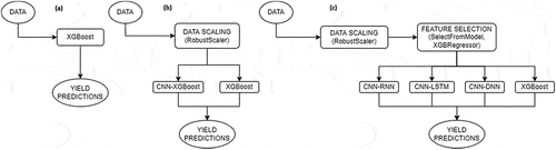
The crop yield prediction depends on multiple factors and thus, the execution speed of the model is crucial. At the same time, the selection of the most important criteria to estimate crop production is important. For this reason, the performance of the model may vary based on the number of features and samples. Ensemble methods of ML and DL-based techniques can take advantage of different algorithms to increase accuracy, reliability, sustainability, efficient learning, and robustness in building models (Ardabili et al., 2019; Mosavi et al., 2019). For the sake of computation speed and efficiency, the Extreme Gradient Boosting (XGBoost) algorithm was used. In one case, the XGBoost was used without being combined with any other technique. Furthermore, in another scenario, we employed CNN to initially extract the important features to be imported in the XGBoost model for making predictions. Due to CNN’s ability to extract information (Mosavi, Ardabili, and Varkonyi-Koczy 2019), we deployed another hybrid model that consists of a CNN followed by a DNN and a Fully Connected (FC) layer (see Appendix A). Lastly, because of the time-series data, we employed hybrid models of CNN layers combined with either RNN or LSTM layers. RNN and LSTM layers can handle time-series data while also benefiting from feedback connections (Mosavi, Ardabili, and Varkonyi-Koczy 2019) as in our case where we worked with data per location and year. Figure 1 shows the visual representation of the proposed models.

Figure 1. A visual representation of the proposed models: (a) XGBoost (raw), (b) CNN-XGBoost (with RobustScaler) and XGBoost (with RobustScaler), (c) CNN-RNN (with RobustScaler and SelectFromModel), CNN-LSTM (with RobustScaler and SelectFromModel), CNN-DNN (with RobustScaler and SelectFromModel), XGBoost (with RobustScaler and SelectFromModel).

Hyperparameters, evaluation metrics, and libraries

We experimented on tuning the hyperparameters and the depth of the models. The XGBoost model depends on several parameters. Amongst others, we tuned the maximum depth of a tree, while tuning the shrinkage used in the update to prevent overfitting. Setting lower values to both of them prevents the model from overfitting the data. We also tuned the minimum loss reduction required to make a further partition on a leaf node of the tree, and the minimum sum of instance weight needed in a child. If those parameters are set with larger values, overfitting can be avoided. Lastly, the subsample ratio of the training instances and subsample ratio of columns when constructing each tree were tuned. Lower ratios of those subsamples are used when overfitting takes place.

As for the CNN and DNN branches of the hybrid models, they were both built with stacked convolutional and dense layers, respectively. Moreover, experiments were performed on the number of nodes, the learning rate, and the batch size, while we applied an early stopping criterion as a callback to avoid overfitting. In order to evaluate the performance of our model, we used the following evaluation metrics: Mean Squared Error (MSE), Root Mean Squared Error (RMSE), Mean Absolute Error (MAE), Coefficient of determination (R²). The MSE is the squared difference of the observed values of a variable with its predicted values, divided by the number of values for this variable (Equation 1(1) $MSE=\frac{1}{n}{\sum }_{i=1}^n{\left(y_i-{\hat{y}}_i\right)}^2$(1) ). It is an assessment of the quality of the predictor. The RMSE is the square root of the MSE, indicating the standard deviation of the residuals (prediction errors) (Equation 2(2) $RMSE=\sqrt{\frac{1}{n}{\sum }_{i=1}^n{\left(y_i-{\hat{y}}_i\right)}^2}$(2) ).

(1) $MSE=\frac{1}{n}{\sum }_{i=1}^n{\left(y_i-{\hat{y}}_i\right)}^2$(1)

(2) $RMSE=\sqrt{\frac{1}{n}{\sum }_{i=1}^n{\left(y_i-{\hat{y}}_i\right)}^2}$(2)

The absolute difference of the predicted value with the actual value defines the MAE, which is a measure of errors between paired observations expressing the same phenomenon (Equation 3(3) $MAE=\frac{1}{n}{\sum }_{i=1}^n\left|{\hat{y}}_i-y_i\right|$(3) ).

(3) $MAE=\frac{1}{n}{\sum }_{i=1}^n\left|{\hat{y}}_i-y_i\right|$(3)

Lastly, the R² is the proportion of the variation in the dependent variable that is predictable from the independent variables. It is expressed by the division of Sum of Squares of Residuals (SS_Res) with the total Sum of Squares (SS_Tot), and it ranges between 0 and 1 (Equation 4(4) $R^2=1-\frac{{\sum }_i{\left(y_i-{\hat{y}}_i\right)}^2}{{\mathrm{\Sigma }}_i\left(y_i-\frac{1}{n}{\sum }_{i=1}^n{y}_i\right)}$(4) ).

(4) $R^2=1-\frac{{\sum }_i{\left(y_i-{\hat{y}}_i\right)}^2}{{\mathrm{\Sigma }}_i\left(y_i-\frac{1}{n}{\sum }_{i=1}^n{y}_i\right)}$(4)

All the experiments were performed in Python on the platform of Google Colab using multiple libraries and working with the Tensorflow framework as backend and Keras as frontend. The experiments in the Google Colab platform were carried out with Python version 3.7.10, Tensorflow version 2.4.1, and Keras version 2.4.3. The main libraries used are Pandas, sci-kit learn, Numpy, and Matplotlib.

Experimental results

In this section, the results of our research are presented. Before training the model and making predictions, we performed feature engineering on the dataset to select the most important features. Initially, we employed the hybrid CNN-XGBoost model where the CNN algorithm consists of three convolutional layers followed by a max-pooling and a dropout layer. The whole dataset with all features was imported to the first convolutional layer using a reshape layer so that they could be used by the CNN. After the dropout layer, the data were flattened and imported into a Fully Connected (FC) layer with a Rectified Linear Unit (ReLU) activation function. The dense layer of the FC from which the features were extracted consists of 48 nodes. Hence, 48 features were used to train the XGBoost model and make predictions.

Subsequently, the XGBoost was employed as a single method for training and making predictions. The whole dataset was used including all growing seasons and locations. The XGBoost alone was able to normalize and select the most important features. As such, we imported the complete dataset into the XGBoost model and got almost the same fit, but with worse evaluation performance, as shown in Table 1. In an attempt to make our approach much simpler and more efficient by reducing the number of imported features, we, then, used the XGBoost model with both the RobustScaler and combined it with the SelectFromModel feature selection technique. In the first case, it performed slightly worse than the hybrid CNN-XGBoost model, as shown in Table 1. In the second case, the XGBoost model was used as the estimator attribute of the feature selection method. This method selected one-fourth of the total features and presented the second-best result, as shown in Table 1.

Table 1. Performance of proposed models with respect to different evaluation metrics

Models	RMSE	MSE	MAE	R^2
CNN-DNN (with RobustScaler and SelectFromModel)	0.266	0.071	0.199	0.87
CNN-XGBoost (with RobustScaler)	0.346	0.120	0.263	0.78
XGBoost (raw)	4.936	24.360	3.764	0.80
XGBoost (with RobustScaler)	0.337	0.113	0.259	0.79
XGBoost (with RobustScaler and SelectFromModel)	0.299	0.089	0.228	0.83
CNN-LSTM (with RobustScaler and SelectFromModel)	0.415	0.172	0.314	0.67
CNN-RNN (with RobustScaler and SelectFromModel)	0.350	0.123	0.269	0.77

Furthermore, the hybrid CNN-DNN model consists of three stacked convolutional layers, followed by batch normalization, a max-pooling, and a dropout layer. The first CNN layer includes 64 neurons, while the second one has 128 and the third one has 256 neurons. The features imported in the first convolutional layer were selected with the SelectFromModel feature selection technique and the XGBoost as the estimator. The outputs of the convolution were then flattened and imported into a DNN built with three dense layers and ending in a dropout layer. The dense layers include the same number of neurons as the CNN layers (i.e., 64, 128, 512). Then, an FC layer is followed with a linear activation function to provide the predictions. This model presented the best performance amongst the other models, as shown in Table 1.

Lastly, the same architecture as the hybrid CNN-DNN model followed the hybrids CNN-RNN and CNN-LSTM models. Instead of DNN, they consist of three stacked RNN and LSTM layers, respectively. All data were normalized with the RobustScaler scaling technique before being further processed, except for one case of applying XGBoost as a single method. The performance is evaluated in terms of the RMSE, MSE, MAE, and R² metrics. For RMSE, MSE, and MAE the lower the score value is, the performance is better. As for the R², the higher the value is, the predictions better fit the original data.

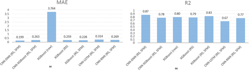
According to the results, the hybrid CNN-DNN model with normalization and feature selection techniques achieved a remarkable performance, having R² of 0.87, RMSE of 0.266, MSE of 0.071, and MAE of 0.199. The model performance resulted after running the model in 150 epochs, as shown in Figure 2. Figure 3 depicts MSE (on the Left) and RMSE (on the Right) values for the proposed models. Figure 4 shows MAE (on the Left) and R² (on the Right) values for the proposed models.

Figure 2. The performance of hybrid CNN-DNN in terms of the ratio of loss (MSE) per epoch.

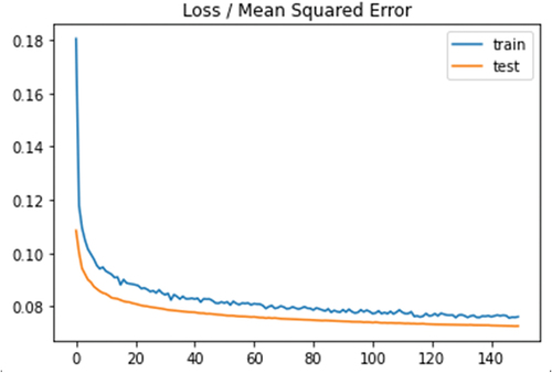
Figure 3. MSE and RMSE values for all the proposed models.

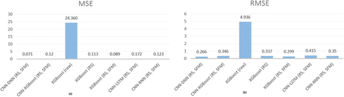
Figure 4. MAE and R² values for all the proposed models.

Discussion

In this study, we used all years and locations of data to train the models and make predictions. Unfortunately, it was not possible to reproduce the results of Khaki, Wang, and Archontoulis (2020) through the code script provided due to incompatible versions of libraries and implementation frameworks. They also concluded that their CNN-RNN model can achieve a performance of R² within the range of 85.45–87.09%, combined with an RMSE in the range of 4.15–4.91. In our research, the CNN-RNN model performed slightly worse (R² = 77%, RMSE = 0.350), while two of our proposed models showed almost similar results with less computational resources, less complexity, and more specialized techniques. Our proposed CNN-DNN outperformed with R² = 87% and RMSE = 0.266, and our XGBoost-based model was the second-best model with R² = 83% and RMSE = 0.299. The results of our outperforming CNN-DNN model indicate the novelty of our research for dealing with such a large dataset by using the proper data processing methods, architecture, and hyperparameter values. This model helped us achieve their highest performance in terms of R², but we have also reached much lower RMSE. As for our second-best proposed model, the XGBoost achieved an R² slightly worse than theirs, but still with less RMSE, computational resources, complexity, and higher speed.

Our approach could prove to be more efficient in making predictions because outliers or features with large variance through the years and different locations can be used to make an estimation. In their article, Khaki, Wang, and Archontoulis (2020) used a much lower learning rate of 0.0003, a higher batch size of 25, and thousands of epochs. However, with respect to memory and time limitation, we used a learning rate of 0.005, a batch size of 12 and 150 epochs with a callback for early stopping. It is worth mentioning the different performances that we obtained from all the models when using different scaling techniques and applying a feature selection method. We consider that choosing a scaling technique should count on the different units and variance of the data. In our case where there are 395 different features with different values range and units, there was the need to capture the outliers that had an impact on features’ variance. That is why the RobustScaler technique proved to be better than the others. As for the feature selection method, it was crucial to use a light and efficient model for selecting features. This is the reason why using an XGBoost model for feature selection would be the best choice. XGBoost with its gradient boosting specialty is one of the most used algorithms handling large and complex datasets with high performance in a short time.

The reason behind combining several state-of-the-art algorithms to build hybrid models was to explore their applicability in handling such a large dataset that consists of plenty of independent variables. The advantages and disadvantages of using each method are presented in Table 2. The methods were compared based on their accuracy and complexity level and in terms of speed. The major advantage of the XGBoost stands on its high speed and accuracy at the same time. Probably that is because of its architecture which was designed for high-speed and performance in both classification and regression tasks by employing gradient boosted decision trees (Brownlee 2018). Moreover, it has the ability to boost trees for high model performance and speed (Quinto 2020), while constructing trees in parallel to deal with very large datasets. The XGBoost added those advantages to the hybrid model of CNN-XGBoost, which had the advantages of computation speed, but lacked accuracy. Also, the complexity was higher when one or more DL algorithms were used, making DL algorithms difficult to handle and tune. Methods like LSTM and RNN showed very low performance in both speed and accuracy. It seems that their abilities to handle time slow them down. That comes to the dilemma of whether to choose an ML or a DL method. Apparently, the answer stands between the accuracy that needs to be achieved and the resources that can be used. The more complex a method does not necessarily mean much higher performance.

Table 2. Advantages and disadvantages for each method based on a scoring system of “+” for sufficient level and “++” for the high level of each case

Models	Accuracy	Speed	Complexity
CNN-DNN (with RobustScaler and SelectFromModel)	++	+	++
CNN-XGBoost (with RobustScaler)	+	+	++
XGBoost (raw)	+	++
XGBoost (with RobustScaler)	+	++
XGBoost (with RobustScaler and SelectFromModel)	++	++	+
CNN-LSTM (with RobustScaler and SelectFromModel)			++
CNN-RNN (with RobustScaler and SelectFromModel)	+		++

However, results may differ in each run of the code. This happens because of the stochastic nature of the algorithms, meaning that the behavior of the algorithm incorporates elements of randomness every time, given the same dataset. Another reason is that all years and locations are used, resulting in a different sample every time we train the model. As a result, the algorithms learn a slightly different model in each turn, making slightly different predictions, evaluations, and performance.

Conclusion

In this study, we investigated a combination of machine learning and deep learning algorithms for estimating crop production and built hybrid models. The dataset was referred to as soybean crop across the Corn Belt in the United States and was previously used in many studies. Also, the dataset consists of weather, soil, and farm management data. We proposed five approaches by taking advantage of specific ML and DL algorithms’ specialties. The proposed approaches are the XGBoost as a single model, the XGBoost with scaling, the XGBoost combined with scaling and feature selection methods, the hybrids CNN-XGBoost, CNN-DNN, CNN-RNN, and CNN-LSTM models. The XGBoost was also used as an estimator for the feature selection technique. We took advantage of the speed and efficiency of XGBoost while using CNN to capture the dependencies of the data and extract information out of the data. The DNN was used as a feed-forward propagation method for making predictions. The hybrid CNN-DNN model outperformed all the others, having R² = 0.87, RMSE = 0.266, MSE = 0.071, and MAE = 0.199. Although we set a variance threshold and performed feature selection to explain what features should be used, there is still room for future research to make the models more explainable. It should be possible to explain in more detail how and what features were selected.

One limitation of this work is the use of the dataset that belongs to the soybean crop across the Corn Belt in the United States. Our results might be slightly different if different datasets are evaluated using the proposed models. The limited computational resources for free usage in the platform of Google Colab is another limitation for experimenting with different architectures, epochs, and hyperparameter values that slows down our model creation process. There is also a possibility to make the feature selection more distinct if the variables in the dataset are provided with their names instead of indices per category.

We consider that our study contributes to making predictions with simpler and state-of-the-art ML and DL algorithms by taking advantage of their special attributes. We demonstrated that high performance can be achieved with ensemble methods of ML and DL by taking advantage of the algorithms, architecture, hyperparameter values, and data processing. Simple models can prove to be efficient and overcome time limitations for fast predictions to support decision-making. Moreover, XGBoost is a promising ML method for both classification and regression tasks, performing very well in most cases. In our study, one of the XGBoost models presented the second-best performance. A hybrid model of XGBoost with a DL algorithm like RNN or LSTM, combined with an attention mechanism may provide higher performance in crop yield prediction using sequential data of dates, this is a future work we may analyze. Lastly, transfer learning can be used with a pre-trained model on a similar regression task for crop yield prediction. This method can save a lot of computational resources.

Code availability

Source code is available upon request

Ethical consideration

The study did not involve humans or animals

Acknowledgments

Open Access funding provided by the Qatar National Library.

Disclosure statement

No potential conflict of interest was reported by the author(s).

Data availability statement

The research uses publicly available data.https://github.com/saeedkhaki92/CNN-RNN-Yield-Prediction

Appendix A.

Hybrid CNN-DNN model architecture

References

- Apolo-Apolo, O. E., J. Martínez-Guanter, G. Egea, P. Raja, and M. Pérez-Ruiz. 2020a. Deep learning techniques for estimation of the yield and size of citrus fruits using a UAV. European Journal of Agronomy 115:126030. doi:10.1016/j.eja.2020.126030.
- Apolo-Apolo, O. E., M. Pérez-Ruiz, J. Martínez-Guanter, and J. Valente. 2020b. A cloud-based environment for generating yield estimation maps from apple orchards using UAV imagery and a deep learning technique. Frontiers in Plant Science 11. doi:10.3389/fpls.2020.01086.
- Ardabili, S., A. Mosavi, and A. R. Várkonyi-Kóczy. 2019. Advances in machine learning modeling reviewing hybrid and ensemble methods. In International Conference on Global Research and Education, 215–1950. Cham: Springer. September.
- Bargoti, S., and J. P. Underwood. 2017. Image segmentation for fruit detection and yield estimation in apple orchards. Journal of Field Robotics 34 (6):1039–60. doi:10.1002/rob.21699.
- Bellocchio, E., T. A. Ciarfuglia, G. Costante, and P. Valigi. 2019. Weakly supervised fruit counting for yield estimation using spatial consistency. IEEE Robotics and Automation Letters 4 (3):2348–55. doi:10.1109/LRA.2019.2903260.
- Bengio, Y. 2009. Learning deep architectures for AI. Delft, The Netherlands: Now Publishers Inc.
- Brownlee, J. 2018. XGBoost with Python. Victoria, Australia: Machine Learning Mastery Pty.
- Buduma, N., and N. Locascio. 2017. Fundamentals of deep learning: Designing next-generation machine intelligence algorithms. Sebastapol, CA, USA: O’Reilly Media, Inc.
- Cabrera, V. E., D. Solís, G. A. Baigorria, and D. Letson. 2009. Managing climate variability in agricultural analysis. In Ocean circulation and El Niño: New research, edited by John A. Long and David S. Wells 163–79. Hauppauge, NY: Nova Science Publishers, Inc.
- Chlingaryan, A., S. Sukkarieh, and B. Whelan. 2018. Machine learning approaches for crop yield prediction and nitrogen status estimation in precision agriculture: A review. Computers and Electronics in Agriculture 151:61–69. doi:10.1016/j.compag.2018.05.012.
- Coviello, L., M. Cristoforetti, G. Jurman, and C. Furlanello. 2020. GBCNet: In-field grape berries counting for yield estimation by dilated CNNs. Applied Sciences 10 (14):4870. doi:10.3390/app10144870.
- Desa, U. (2016). Transforming our world: The 2030 agenda for sustainable development.
- Elavarasan, D., and P. M. D. Vincent. 2020. Crop yield prediction using deep reinforcement learning model for sustainable agrarian applications. IEEE Access 8:86886–901. doi:10.1109/ACCESS.2020.2992480.
- Filippi, P., E. J. Jones, N. S. Wimalathunge, P. D. S. N. Somarathna, L. E. Pozza, S. U. Ugbaje, and T. F. A. Bishop. 2019. An approach to forecast grain crop yield using multi-layered, multi-farm data sets and machine learning. Precision Agriculture 20 (5):1015–29. doi:10.1007/s11119-018-09628-4.
- Gao, Y., S. Wang, K. Guan, A. Wolanin, L. You, W. Ju, and Y. Zhang. 2020. The ability of sun-induced chlorophyll fluorescence from OCO-2 and MODIS-EVI to monitor spatial variations of soybean and maize yields in the Midwestern USA. Remote Sensing 12 (7):7. doi:10.3390/rs12071111.
- Hani, N., P. Roy, and V. Isler. 2020. A comparative study of fruit detection and counting methods for yield mapping in apple orchards. Journal of Field Robotics 37 (2):263–82. doi:10.1002/rob.21902.
- Herrero-Huerta, M., P. Rodriguez-Gonzalvez, and K. M. Rainey. 2020. Yield prediction by machine learning from UAS-based multi-sensor data fusion in soybean. Plant Methods 16 (1):1–16. doi:10.1186/s13007-020-00620-6.
- Kang, Y., M. Ozdogan, X. Zhu, Z. Ye, C. Hain, and M. Anderson. 2020. Comparative assessment of environmental variables and machine learning algorithms for maize yield prediction in the US Midwest. Environmental Research Letters 15 (6):064005. doi:10.1088/1748-9326/ab7df9.
- Khaki, S., and L. Wang. 2019. Crop yield prediction using deep neural networks. Frontiers in Plant Science 10. doi:10.3389/fpls.2019.00621.
- Khaki, S., L. Wang, and S. V. Archontoulis. 2020. A CNN-RNN framework for crop yield prediction. Frontiers in Plant Science 11: 1750.
- Kim, N., K.-J. Ha, N.-W. Park, J. Cho, S. Hong, and Y.-W. Lee. 2019. A comparison between major artificial intelligence models for crop yield prediction: Case study of the midwestern United States, 2006–2015. ISPRS International Journal of Geo-Information 8 (5):240. doi:10.3390/ijgi8050240.
- Lal, R. 2016. Feeding 11 billion on 0.5 billion hectare of area under cereal crops. Food and Energy Security 5 (4):239–51. doi:10.1002/fes3.99.
- LeCun, Y., Y. Bengio, and G. Hinton. 2015. Deep learning. Nature 521 (7553):436–44. doi:10.1038/nature14539.
- Lin, T., R. Zhong, Y. Wang, J. Xu, H. Jiang, J. Xu, Y. Ying, L. Rodriguez, K. C. Ting, and H. Li. 2020. DeepCropNet: A deep spatial-temporal learning framework for county-level corn yield estimation. Environmental Research Letters 15 (3):034016. doi:10.1088/1748-9326/ab66cb.
- Ma, J. W., C. H. Nguyen, K. Lee, and J. Heo. 2019. Regional-scale rice-yield estimation using stacked auto-encoder with climatic and MODIS data: A case study of South Korea. International Journal of Remote Sensing 40 (1):51–71. doi:10.1080/01431161.2018.1488291.
- Maimaitijiang, M., V. Sagan, P. Sidike, S. Hartling, F. Esposito, and F. B. Fritschi. 2020. Soybean yield prediction from UAV using multimodal data fusion and deep learning. Remote Sensing of Environment 237:111599. doi:10.1016/j.rse.2019.111599.
- McGuire, S. 2015. FAO, IFAD, and WFP. In The state of food insecurity in the world 2015: Meeting the 2015 international hunger targets: Taking stock of uneven progress. Rome: FAO. Oxford University Press.
- Meng, X., M. Liu, and Q. Wu. 2020. Prediction of rice yield via stacked LSTM. International Journal of Agricultural and Environmental Information Systems (IJAEIS) 11 (1):86–95. doi:10.4018/IJAEIS.2020010105.
- Moghimi, A., C. Yang, and J. A. Anderson. 2020. Aerial hyperspectral imagery and deep neural networks for high-throughput yield phenotyping in wheat. Computers and Electronics in Agriculture 172:105299. doi:10.1016/j.compag.2020.105299.
- Mosavi, A., S. Ardabili, and A. R. Varkonyi-Koczy. 2019. List of deep learning models. In International Conference on Global Research and Education, 202–14. Cham: Springer. September.
- Quinto, B. (2020). Next-Generation Machine Learning with Spark. Berlin, Germany: Apress.
- Saravi, B., A. P. Nejadhashemi, and B. Tang. 2020. Quantitative model of irrigation effect on maize yield by deep neural network. Neural Computing & Applications 32 (14):10679–92. doi:10.1007/s00521-019-04601-2.
- Shahhosseini, M., R. A. Martinez-Feria, G. Hu, and S. V. Archontoulis. 2019. Maize yield and nitrate loss prediction with machine learning algorithms. Environmental Research Letters 14 (12):124026. doi:10.1088/1748-9326/ab5268.
- Sun, J., L. Di, Z. Sun, Y. Shen, and Z. Lai. 2019. County-level soybean yield prediction using deep CNN-LSTM model. Sensors (Switzerland) 19 (20):4363. doi:10.3390/s19204363.
- Tedesco-Oliveira, D., P. Da Silva, R. W. Maldonado, and C. Zerbato. 2020. Convolutional neural networks in predicting cotton yield from images of commercial fields. Computers and Electronics in Agriculture 171:105307. doi:10.1016/j.compag.2020.105307.
- van Klompenburg, T., A. Kassahun, and C. Catal. 2020. Crop yield prediction using machine learning: A systematic literature review. Computers and Electronics in Agriculture 177:105709. doi:10.1016/j.compag.2020.105709.
- Wang, X., J. Huang, Q. Feng, and D. Yin. 2020a. Winter wheat yield prediction at county level and uncertainty analysis in main wheat-producing regions of China with deep learning approaches.Remote Sensing 12 (11): 1744.
- Wang, Y., Z. Zhang, L. Feng, Q. Du, and T. Runge. 2020b. Combining multi-source data and machine learning approaches to predict winter wheat yield in the conterminous United States. Remote Sensing 12 (8). doi: 10.3390/RS12081232.
- Xu, X., P. Gao, X. Zhu, W. Guo, J. Ding, C. Li, M. Zhu, and X. Wu. 2019. Design of an integrated climatic assessment indicator (ICAI) for wheat production: A case study in Jiangsu Province, China. Ecological Indicators 101:943–53. doi:10.1016/j.ecolind.2019.01.059.
- You, J., X. Li, M. Low, D. Lobell, and S. Ermon (2017). Deep Gaussian process for crop yield prediction based on remote sensing data. In Paper presented at the Thirty-First AAAI conference on artificial intelligence, San Francisco, California, USA.
- Zhang, D. 2006. Advances in machine learning applications in software engineering. Hershey, PA, USA: Igi Global.
- Zhou, C. Q., J. Hu, Z. F. Xu, J. B. Yue, H. B. Ye, and G. J. Yang. 2020. A monitoring system for the segmentation and grading of broccoli head based on deep learning and neural networks. Frontiers in Plant Science 11:13. doi:10.3389/fpls.2020.00402.