Brain Tumor Classification Based on Hybrid Optimized Multi-features Analysis Using Magnetic Resonance Imaging Dataset

ABSTRACT

Brain tumors are deadly but become deadliest because of delayed and inefficient diagnosis process. Large variations in tumor types also instigate additional complexity. Machine vision brain tumor diagnosis addresses the problem. This research’s objective was to develop a brain tumor classification model based on machine vision techniques using brain Magnetic Resonance Imaging (MRI). For this purpose, a novel hybrid-brain-tumor-classification (HBTC) framework was designed and evaluated for the classification of cystic (cyst), glioma, meningioma (menin), and metastatic (meta) brain tumors. The proposed framework lessens the inherent complexities and boosts performance of the brain tumor diagnosis process. The brain MRI dataset was input to the HBTC framework, pre-processed, segmented to localize the tumor region. From the segmented dataset Co-occurrence matrix (COM), run-length matrix (RLM), and gradient features were extracted. After the application of hybrid multi-features, the nine most optimized features were selected and input to the framework’s classifiers, namely multilayer perception (MLP), J48, meta bagging (MB), and random tree (RT) to classify cyst, glioma, menin, and meta tumors. Maximum brain tumor classification performance achieved by the HBTC framework was 98.8%. The components and performance of the proposed framework show that it is a novel and robust classification framework.

Introduction

In the twenty-first century, no doubt, people’s living standards, technology paradigms, healthcare facilities, and infrastructure have improved remarkably where computing and information technology have grabbed all over the other fields like an octopus (Patel, Patel, and Scholar 2016). Besides the developments, humankind is still facing several problems such as poverty, hunger, food, terrorism, water, diseases, climate change, and environmental pollution. Many fatal diseases are harming people like cancer, hepatitis, diabetes, heart problems, tuberculosis, and Alzheimer’s (Bloom and Cadarette 2019).

The tumor is the deadliest one among ten highly ranked diseases worldwide which may damage many specific parts of the human body like lungs, liver, stomach, spinal cord, or brain. By the annual report of 2018 of the International Agency for Research on Cancer (IARC), number of tumor deaths and incoming expected cases were in millions (Ferlay et al. 2021; Sung et al. 2021). Our body comprises 37.5 trillion cells, where only the brain has 100 billion neurons and one trillion glial cells (Bianconi et al. 2013; von Bartheld, Bahney, and Herculano-Houzel 2016). The abnormal growth of these cells is called a tumor or neoplasm and categorized as benign (non-cancerous) or malignant (cancerous). A malignant tumor grows to the other body parts, but a benign tumor stays at a specific region (Sinha 2018).

Brain is the most fundamental part of our body, composed of massive soft tissues and layers, connected to the spinal cord by nerve cells, making up the central nervous system (CNS) which controls all the physical, mental, emotional, or even spiritual functionalities of our body by farming a rapid and continuous communication network of neurons between brain and spinal cord. The complete nervous system is made of CNS and peripheral nervous system (PNS) (Wahid, Fayaz, and Shah 2016). Unfortunately, such an important and complex structure may also suffer from tumors. Brain tumors are the common cause of deaths around the world and affect people regardless of age, sex, and race. In 2020, International Agency for Research on Cancer (IARC) and GLOBOCAN observed 251,329 brain tumor deaths and estimated 308,102 new cases (Ferlay et al. 2021; Sung et al. 2021).

Two main categories of brain tumors are primary and secondary or benign and malignant. Primary brain tumors start within the brain and stay there, but secondary tumors are the cancer cells that grow from other parts of the body. Benign tumors grow slowly and expose distinct borders, and they are removed depending on the regions of the brain where they locate. On the contrary, malignant brain tumors are fast-growing and harmful and do not show clear and precise edges because of their creeping root tendency to the nearby tissues. There are almost more than 120 brain tumors, but glioma, meningioma, and metastatic are the most frequently occurring brain tumors (D.N. et al. 2016; Sinha 2018).

Doctor’s clinical trials for elementary diagnosis include physical examination, biography, digital screening, and biopsy tests. The objectives are to locate the abnormal tissues’ location, region, and orientation. After physical examination and memoir, the next task is brain imaging. Brain imaging is critical since the brain comprises very sensitive and delicate tissues. There exist various medical imaging modalities, but MRI works well on soft tissues and is the best tool to detect abnormalities in brain tissues. Other imaging tools include Computed tomography (CT), perfusion MRI, functional MRI, positron emission tomography (PET), or flu-orthodoxy-glucose positron emission tomography/computed tomography (FDG-PET/CT). Timely and accurate identification of the site and status of a brain tumor can steer to effective treatment, including chemotherapies or surgeries, depending upon the condition (Chourmouzi et al. 2014; Perkins,A. Liu 2016; J Strong and Garces 2016).

Manual diagnosis of brain tumors is tedious, delayed, qualitative, and imprecise; in contrast, we need an early and accurate quantitative diagnosis to save lives. Additionally, doctors also require the precise quantification of the tumor region for specific treatment (Perkins and Liu 2016; Wahid, Fayaz, and Salam Shah 2016).

Nowadays large arrays of MV techniques have been employed for data mining and classification in diverse fields. These include bioinformatics, agro-informatics, social sciences, robotics, etc. (Batchelor 2012a). Many MV techniques have recently evolved to develop automated brain tumor classification systems that assist radiologists and doctors for early and accurate diagnosis. Two primary objectives of these techniques are to segment and classify brain tumors. This research focused on developing a novel and robust machine vision system for automatic diagnosis and classification of brain tumors incorporating hybrid optimized multi-features analysis and machine vision classifiers to classify the four brain tumors using brain MRI scans (Batchelor and Whelan 2012; El-Dahshan et al. 2014; Gonzalez 2018; Wahid, Fayaz, and Salam Shah 2016).

Major contributions in this research study are the acquisition of MRI dataset from the RD-BVH, hybrid multi-features optimization and implementation of HBTC framework.

Literature Review

From near past to recent, many researchers have been devoted in segmenting and classifying brain MRIs. This section provides a quick overview of some of the previous newer and the state-of-the-art approaches.

Arunkumar with his research fellows developed an outstanding brain tumor classification model based on classic machine vision approaches including Fourier transform image enhancement, fully automated trainable segmentation, histogram-of-oriented-gradients (HOG) feature extraction, ANN-based classification model. Non-ROI brain components are filtered using size, circularity and gray-dcale average. The developed model classified normal and abnormal brain slices with overall 92.14% classification accuracy using k-fold-cross validation method (Arunkumar et al. 2020).

Sarah and research participants made a comparative analysis of the two brain tumor segmentation algorithms namely active-counter and ostu-threshold. Multimodel-Brain-Tumor-Image-Segmentation (BRATS) benchmark brain MRI dataset is used in this comparative analysis. Both algorithms were implemented using MATLAB and their similarity coefficients were evaluated by Dice, BFScore, and Jaccard evaluations. Results showed that similarity index of active-counter was higher than the ostu-threshold (Husham et al. 2021).

Mallikarjan, with his research fellows, proposed a brain tumor classification system to classify benign and malignant tumors. Region-growing was used for segmentation, and center-symmetric-level-binary-pattern (CSLBP) and gray-level-run-length matrix (GLRLM) features were fused, and the system gained noteworthy classification accuracy (Mudda, Manjunath, and Krishnamurthy 2020a).

Santhosh and his fellows presented a classification model to classify normal and abnormal brain tissues. The system was based on threshold and watershed segmentation. SVM gave overall classification accuracy up to 85.32% (Seere and Karibasappa 2020).

Hafeez Ullah and research fellows proposed a brain tumor classification model based on brain MRIs, acquired from RD-BVH. Intensity, shape and texture features were extracted from brain MRI slices and the proposed methology gained overall 97% classification accuracy (Ullah, Batool, and Gilanie 2018).

Rafael, with other researchers, suggested a system to classify glioblastoma and metastatic. First- and second-order statistics features were extracted, and Interclass-correlation-coefficient (ICC) was applied for feature reduction. support vector machine (SVM) gave 89.6% accuracy rate for area-under-the-curve (AUC) (Ortiz-Ramón et al. 2020).

Gupta and Sasidhar described a brain tumor classification model to classify low-grade and high-grade brain tumors. Ostu-thresholding was used for segmentation and 18 Segmentation-Based Fractal Texture Analysis (SFTA) features were input to SVM which gave 87% accuracy (Gupta and Sasidhar 2020).

In another research study, Gilani with his research fellows acquired brain MRI datasets from RD-BVH and Harvard Medical School (HMS), and suggested a brain tumor cross-validation train-test classification model, based on multiple texture parameters. The model achieved classification accuracies for different categories ranging from 86% to 92% (Gilanie et al. 2019).

Zacharacki, with his coauthors, proposed a brain tumor classification and grading system using machine learning techniques. Gliomas, meningioma, glioblastoma, and metastases were classified in a binary manner. Statistical features were extracted and optimized using rank-based criteria. Classification accuracies were notable using 3-fold-cross-validation (Zacharaki et al. 2009).

Marco, with his fellows, proposed a model to classify benign and malignant brain tumors. Brain images were segmented using adaptive thresholding. Fast Fourier transform (FFT) features were extracted and then optimized by minimal-redundancy-maximal-relevance (MRMR). Finally, SVM was applied to classify brain images into normal and abnormal (Alfonse and Salem 2016).

Mohsin, with his companion researchers, suggested a hybrid machine learning model for brain tumor identification. Segmentation was based on a feedback pulse-coupled neural network, and wavelet features were extracted. Feedforward backpropagation neural networks remarkably classified the brain images (Mohsen, El-Dahshan, and Salem 2012).

With fellow researchers, Selvaraj proposed a least-square-support-vector-machine (LS-SVM) based classification model to classify normal and abnormal brain MRI scans. Different statistical features, including GLCM features, were extracted. LS-SVM gave the highest results compared with K-nearest neighbor, MLP, and radial-basis-function (RBF) (Selvaraj et al. 2007).

Tiwari, with his coauthors, presented a model to classify meningioma and astrocytoma. Features including GLCM and GLRLM were extracted from ROIs. Firstly, 263 features were extracted, then 108 Laws texture energy measures (LTEM) features were added. Multilayered ANN gave results between 78.10% and 92.43% (Tiwari et al. 2017).

Salama and research fellows introduced a novel Multiple Features Evaluations Approach (MFEA) method to improve the Parkinson’s diagnosis process based on classification of voice variations. MFEA used five feature selection agents, each giving the dominant features. Features obtained by all agents are then combined to form the optimal features set. Next, multiple classifiers are evaluated on the original features and the filtered optimal features set. Neural network gave maximum performance on the original features where Random Forest gave the maximum 99.49% classification accuracy using a 10-fold-cross-validation method (Mostafa et al. 2019).

Anter and Aboul described a liver tumor classification system to classify benign and malignant tumors. Feature vector comprised GLCM, LBP, SFTA, first-order statistics (FOS), and fused feature (FF). SVM, RF, artificial neural network (ANN), and KNN were applied using a cross-validation method to classify tumors (Anter and Hassenian 2018).

M.A. Mohammed with colleague researchers proposed a breast cancer classification model. The model was based on the classical SFTA (segmentation-based fractal texture analysis) feature extraction method and ANN. Multi-fractal dimension features sets were created for 72 normal and 112 abnormal images. The method applied two-threshold-binary-decomposition (TTBD) and marginal boundaries to compute 12 fractal dimension sets. Next, ANN gave the noteworthy classification accuracy (Mohammed et al. 2018).

Dilliraj, with his coauthors, demonstrated different brain tumor segmentation approaches. Advanced Fuzzy C-Means, self-organizing map, and k-means algorithms were applied to compute the tumor region (Dilliraj, Vadivu, and Anbarasi 2014).

George and Manuel classified four grades of astrocytoma. For preprocessing, pulse coupled neural network and median filter were applied, and fuzzy c-means (FCM) were used for segmentation. First-order and second-order statistical features were reduced to 14 optimized features, which then were input to a deep neural network (DNN) and got 91% accuracy (George and Manuel 2019).

A deep learning scheme was designed by Heba and research team to classify four brain tumor classes namely normal, glioblastoma, sarcoma and metastatic bronchogenic carcinoma. Feature extraction was combined with discrete wavelet transform (DWT) and principal components analysis (PCA). Classifications were performed by deep neural network with seven hidden layers using 7-fold-cross-validation. The model gained overall 96.97% classification rate (Mohsen et al. 2018)

Bhanumathi and Sangeetha proposed a model to classify glioma, acoustic neuroma, and meningioma. In the study, 20 normal and 30 infected images were taken. Convolutional neural network (CNN) models were used for classification where GoogLeNet gave the best accuracy (Bhanumathi and Sangeetha 2019).

Gumaei, with his companion researchers, proposed a classification model using regularized extreme learning machine (RELM) to discriminate between benign and malignant brain tumors. MRIs of meningioma, glioma, and pituitary were acquired and preprocessed. Feature selection was made using GIST, normalized GIST (NGIST), and PCA-NGIST. Using fivefold cross-validation, RELM gave overall accuracy of 92.6144% (Gumaei et al. 2019).

Many of the described approaches are just based on two-class classification: normal and abnormal. Some lacks the localized tumor dataset and many of the above methodologies needs to improve the precision. Even if deep learning systems boost the precision but these systems have lot of processing overhead for training. Thus, we have introduced a novel hybrid-brain-tumor-classification novel HBTC framework based on hybrid features optimization and multifeatures analysis for the brain tumor classification.

Material and Method

In this research, four brain tumor types, namely, cyst, menin, glioma, and meta, were classified using the proposed HBTC framework. This section describes the mythology of the proposed HBTC framework.

Methodology

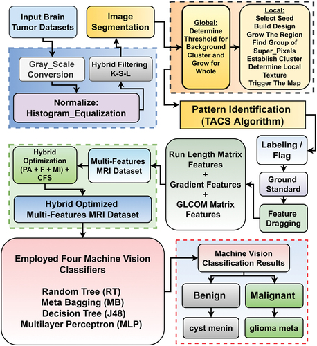
Methodology of the proposed HBTC framework mainly comprises dataset acquisition, pre-processing, segmentation, feature extraction, feature optimization, classification, and evaluation steps. Algorithm 1 presents the procedural steps of the proposed HBTC framework, shown in Table 1. The whole MRI dataset of the four brain tumor types is input in the first step. In the second step, the process entered into a loop. Every image is enhanced by applying a hybrid, Kernel plus Sobel plus Low-pass (K-S-L) filters pre-processing scheme. Next, a tumor region is segmented, and ROIs are created. Next, COM, RLM, and Gradient features are extracted from each segmented ROI, to form a features vector. This process continues until there remain no more unprocessed MRIs. In the third step, a hybrid features optimization technique is applied to obtain the most relevant properties of the images for multi-features analysis. In the fourth step, machine vision classifiers were applied using 10-fold cross-validation on the hybrid optimized features to classify brain tumors. In the fifth step, framework performance was evaluated.

Table 1. Procedural Steps of the HBTC framework

Algorithm 1:Hybrid Brain Tumor Classification Procedure
Begin
Main {	step1: Input ɛ Brain Tumor MRI dataset step2: For 1 to Size-of Brain MRI dataset { Acquire brain tumor MRI Pre-process the input image Segment the tumor region Create segmented ROI Extract RLM, COM, Gradient features } End-For step3: Optimize via (MI + F + PA) + CFS step4: Multi-features analysis & classification step5: Evaluation
}End-Main

The HBTC framework was run using MaZda 4.6 (Strzelecki et al. 2013) and Waikato Environment for Knowledge Analysis (Weka 3.8) (Witten et al. 2016), on Intel(R) Core (TM) i7-8550 U CPU with 16.0 GB of memory and 64-bit operating system of Microsoft Windows 10. The following sections explain each step in detail.

Dataset Acquisition

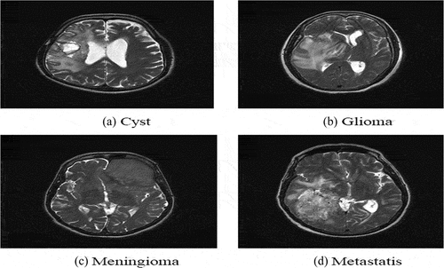
Prime initiative to implement of the HBTC framework was the collection of brain tumor MRI dataset. This section describes the dataset acquision. MRI works well on soft tissues such as the liver, brain, lungs, etc. (Seere and Karibasappa 2020) [18]. For this study, T2-weighted MRI dataset of the four brain tumor types was acquired from MRI machine with specification (OptimaTM MR450w – 70 cm) (Phal et al. 2008). installed in Radiology Department of Bahawal Victoria Hospital (RD-BVH) (Attique et al. 2012; Gilanie et al. 2019; Iqbal 2009; Ullah, Batool, and Gilanie 2018). The sample MRIs of the brain tumors are shown in Figure 1. The dataset comprised 250 patients for each tumor type. Therefore, a total dataset of 1000 (250 × 4) MRIs was collected. The expert radiologist examined and marked all the collected brain MRIs, to ensure the ground truth.

Figure 1. Sample Images of Four Brain Tumor Types.

Pre-Processing

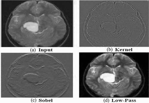
Medical images contain inherent inhomogeneity, poor quality, and noise, thus we need to enhance the quality of the collected brain MR images. This section describes the details of preprocessing federated into the HBTC framework. Preprocessing comprised re-sizing, gray-level conversion, cropping, normalization, and image enhancement. Thus, the acquired MRI datasets were required to enhance. For this study, at the first step, all the collected MRI datasets were converted into the standard format of 8-bit (.bmp) gray-scale and normalized by using histogram equalization. In the second step, the image noise was removed by applying K-S-L image enhancement. (Gonzalez and Rafael 2018; Lakshmi Devasena and Hemalatha 2011). Gradient masks of Sobel filter of size 3 × 3 were applied on the x-axis (Grx) and the other two on the y-axis (Gry), and gradient magnitude (Gr) with its approximation also computed. The effects of applying the filters are shown in Figure 2. Gradient equations are also given below.

(1) $\left|Gr\right|=\sqrt{Gr{x}^2+Gr{y}^2}$(1)

Figure 2. Sample Effects of Image Preprocessing.

Segmentation

Image segmentation is a phase in image processing during which an image is split into various sub-groups according to its properties and features. It reduces the image’s complexity to simplify further processing or analysis. This section discusses segmentation carried out in HBTC framework.

Image segmentation falls into three categories: manual, automated, and semi-automated. Manual segmentation is tedious and error-prone because of human observational variability. Thus, it is used as a golden standard. The semi-automated method solves some problems of manual segmentation by using algorithms but still has limitations. There are diverse forms of semi-automated segmentation that reduce some observational variability, but not all of them (Sachdeva et al. 2013). Automated schemes do not involve users interactively. They fall into two classes: learning-based algorithms and non-learning-based algorithms. Learning approaches rely on training and testing phases, whereas non-learning strategies depend upon image and disease characteristics (Kevin Zhou, Fichtinger, and Rueckert 2019).

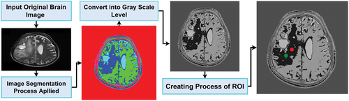
In the HBTC framework, threshold and clustering-based segmentation (TACS) scheme was applied and segmented ROIs were created (Ortiz-Ramón et al. 2020). TACS’s procedural steps are given in Table 2, and its overall model is expressed in Figure 3. Background pixels (B_P) were computed based on a specific threshold value in the first step. The image background was considered a complete cluster based on the threshold. In the next step, the point was determined as a value of base-pixel. This base value of the pixel was used to weigh up all the neighbors of the pixel. With the same approach, the whole image was completed. If the pixel gray intensity value of (P_G) was greater than the B_P value, it was examined as a pixel region of fore-ground (F_P) and grown-up for the whole cluster by determining its R_I (region of interest) or also commonly known as the foreground region.

Table 2. TACS Model

Algorithm 2: threshold and clustering-based segmentation (TACS)
Input:	Brain Image Dataset
Parameter:	MRI Dataset {Brain Image Dataset}
Output:	Clustered Images (C_I) and Region of Interest (R_I)
1. 2. 3. 4. 5. 6. 7. 8. 9. 10. 11. 12. 13. 14. 15. 16. 17. 18.	Function TACS (MRI Dataset) Begin for Total Pixel Measure of whole image (TPM) do B_P ← set threshold for back-ground Pixels P_G ← measure Pixel Gray Intensity T_C_C ← initialize Total_Cluster_Count with 0 if P_G > B_P then T_C_C ← increment Total_Cluster_Count F_G ← calculate fore-ground Pixels R_I ← Region of Interest from image else NOT count Segmentation Area B_P ← calculate Back-ground Pixel end if end for return (C_I, R_I) end Begin end Function

Figure 3. Overall Model of TACS Methodology with taking ROI.

Feature Extraction

This step intends to extract specific properties of the segmented ROIs to discriminate the patterns of input images (Radhakrishnan and Kuttiannan 2012). This section addresses the feature extraction phase of the HBTC framework. The relevant properties are collected into a feature vector to process for the next stage. For texture analysis, we extracted occurrence matrix (COM), run-length matrix (RLM), and gradient features from the segmented ROIs of the brain (Ortiz-Ramón et al. 2020; Tiwari et al. 2017). For this purpose, ROIs of sizes (10 × 10), (15 × 15), and (20 × 20) were created, and 220 COM, 20 RLM, and 5 Gradient features were extracted from each ROI (Anter and Hassenian 2018; Gonzalez and Rafael 2018; Seere and Karibasappa 2020). Thus, three datasets were obtained for experiments. The total feature vector volume (FVV) for each ROI dataset was 490000 (2000 x 245). We performed all Experiments on a machine with processor Core (TM) i7 Intel, 1.8 GHz, containing 16 GB of RAM and a 64-bit operating system of Microsoft Windows 10. Below all the extracted features are described precisely.

Run Length Matrix (RLM)

Galloway proposed this method and is called run-length. It computes the gray or color level runs of various lengths also called length or range of run. Gray or color scales are measured as a multitude of contiguous pixels having the same gray or color scales in a linear fashion. The number of pixels is measured horizontally in four dimensions($0°$,$45°$,$90°$and $135°$). In our study, we extracted 20 RLM features for each image, and matrices of various runs are formulated with respect to each specified θ. We measured short_run_emphasis (S.R.E), long_run_emphasis (L.R.E), gray_level_non_uniformity (G.L.N), gray_level_non_uniformity_normalized (G.L.N.N), run_length_non_uniformity (R.L.N), run_length_non_uniformity_normalized (R.L.N.N), run_percentage (R.P), for each of the segmented ROIs. Below the equations of the used runs are given (Baessler et al. 2020; Mudda, Manjunath, and Krishnamurthy 2020a).

S.R.E describes the determination of short-run lengths distribution, and a larger S.R.E indicates fine and more magnificent textural texture, and its equation is given in Equation 2(2) $S.R.E=\frac{{\sum }_{m=0}^{g_k}{\sum }_{n=1}^{g_r}\frac{\in \left(m,n|\sigma \right)}{n^2}}{g_r\left(\sigma \right)}$(2) )

(2) $S.R.E=\frac{{\sum }_{m=0}^{g_k}{\sum }_{n=1}^{g_r}\frac{\in \left(m,n|\sigma \right)}{n^2}}{g_r\left(\sigma \right)}$(2)

L.R.E describes the measurement of long-run lengths distribution, and larger L.R.E indicates long runs and more rough textures, and its equation is shown in Equation 3(3) $L.R.E=\frac{{\sum }_{m=1}^{g_k}{\sum }_{n=0}^{g_r}\in \left(m,n|\sigma \right){\left(n\right)}^2}{g_r\left(\sigma \right)}$(3) )

(3) $L.R.E=\frac{{\sum }_{m=1}^{g_k}{\sum }_{n=0}^{g_r}\in \left(m,n|\sigma \right){\left(n\right)}^2}{g_r\left(\sigma \right)}$(3)

G.L.N computes similarity factor between gray levels intensities of the given image and a less G.L.N value indicates a more similarity between intensities, and its equation is shown below in Equation 4(4) $G.L.N=\frac{{\sum }_{m=1}^{g_k}{[{\sum }_{n=1}^{g_r}\in \left(m,n|\sigma \right)]}^2}{g_r\left(\sigma \right)}$(4) .

(4) $G.L.N=\frac{{\sum }_{m=1}^{g_k}{[{\sum }_{n=1}^{g_r}\in \left(m,n|\sigma \right)]}^2}{g_r\left(\sigma \right)}$(4)

G.L.N.N is a normalized version of G.L.N with significant quality improvement and it also measures similarity factor between gray level intensities of the given image and a less G.L.N value indicates a more similarity between intensities, and its equation is shown in Equation 5(5) $G.L.N.N=\frac{{\sum }_{m=1}^{g_k}{[{\sum }_{n=1}^{g_r}\in \left(m,n|\sigma \right)]}^2}{g_r{\left(\sigma \right)}^2}$(5) )

(5) $G.L.N.N=\frac{{\sum }_{m=1}^{g_k}{[{\sum }_{n=1}^{g_r}\in \left(m,n|\sigma \right)]}^2}{g_r{\left(\sigma \right)}^2}$(5)

R.L.N computes similarity index between run-lengths of the whole image and a less R.L.N value indicates high homogeneity factor, and its equation is shown in Equation 6(6) $R.L.N=\frac{{\sum }_{n=1}^{g_k}{[{\sum }_{m=1}^{g_r}\in \left(m,n|\sigma \right)]}^2}{g_r\left(\sigma \right)}$(6) .

(6) $R.L.N=\frac{{\sum }_{n=1}^{g_k}{[{\sum }_{m=1}^{g_r}\in \left(m,n|\sigma \right)]}^2}{g_r\left(\sigma \right)}$(6)

R.L.N.N is a normalized version of R.L.N with significant improvement in quality and it also measures similarity factor between run-lengths of the whole image and a less R.L.N.N value indicates high homogeneity factor, and its equation is given below in Equation 7(7) $R.L.N.N=\frac{{\sum }_{m=1}^{g_k}{[{\sum }_{n=1}^{g_r}\in \left(m,n|\sigma \right)]}^2}{g_r{\left(\sigma \right)}^2}$(7) .

(7) $R.L.N.N=\frac{{\sum }_{m=1}^{g_k}{[{\sum }_{n=1}^{g_r}\in \left(m,n|\sigma \right)]}^2}{g_r{\left(\sigma \right)}^2}$(7)

Coarseness of the underlying texture is computed by R.P which is given below in Eq. (8).

(8) $R.P=\frac{g_{r\left(\sigma \right)}}{g_p}$(8)

Co-occurence Matrix (COM)

Co-occurrence matrix (COM) features are also called second-order statistical features, widely used for texture analysis (Haralick, Shanmugam, and Its’Hak 1973). Co-occurrence features measure the dependency and relationship between intensities of neighboring pixels by considering their distances and angles. This method is widely used to discriminate the texture of an underlying image. In this study, four angles:$0°$,$45°$,$90°$and $135°$, are used for each of the eleven second-order co-occurrence features. Obtained features are Energy, Entropy, Sum Entropy, Correlation, Inverse Difference, and Inertia features (Anter and Ella Hassenian 2018; Baessler et al. 2020; Qadri et al. 2019).

Energy measures the homogeneity by computing high-frequency neighboring pairs, and its equation is given below in Equation 9(9) $Enrg=\sum _m\sum _n{\left(m,n\right)}^2\hspace{0.17em}$(9) .

(9) $Enrg=\sum _m\sum _n{\left(m,n\right)}^2\hspace{0.17em}$(9)

Correlation determines the similarity of pixels for some pixel distance in the input image, given in Equation 10(10) $Correlat=\frac{1}{{\rho }_a{\rho }_b}\sum _m\sum _n\left(C-{\omega }_a\right)\left(D-{\omega }_b\right)\left(m,n\right)$(10) .

(10) $Correlat=\frac{1}{{\rho }_a{\rho }_b}\sum _m\sum _n\left(C-{\omega }_a\right)\left(D-{\omega }_b\right)\left(m,n\right)$(10)

Entropy measures the whole content of an image and the neighborhood variability of voxels, and its equation is given in Equation 11(11) $Entrop=-\sum _m\sum _n\left(m,n\right)lo{g}_2\left(m,n\right)\hspace{0.17em}$(11) .

(11) $Entrop=-\sum _m\sum _n\left(m,n\right)lo{g}_2\left(m,n\right)\hspace{0.17em}$(11)

To measure homogeneity at local level in an image the inverse difference is computed, given in Equation 12(12) $Inver{s}_{Diff}=\sum _m\sum _n\frac{\left(m,n\right)}{\left|m-n\right|}$(12) .

(12) $Inver{s}_{Diff}=\sum _m\sum _n\frac{\left(m,n\right)}{\left|m-n\right|}$(12)

To obtain the contrast factor in an image inertia value is quantified and its equation is given in Equation 13(13) $Inert=\sum _m\sum _n{\left(m-n\right)}^2\left(m,n\right)\hspace{0.17em}$(13) .

(13) $Inert=\sum _m\sum _n{\left(m-n\right)}^2\left(m,n\right)\hspace{0.17em}$(13)

Gradient Features

A gradient of an image measures the intensity changes in some fixed or certain directions. Gradient features are given as a two-dimensional vector in which both the directional and magnitude components are computed by taking derivatives for both vertical and horizontal directions. Digital images are represented by discrete values x, y in both directions. It’s a 2D gradient vector containing the largest intensity increment computations in the order and its magnitude as the rate of change, and equations of the four gradient features, namely, Mean, Variance, Skewness, and Kurtosis are given below (Al-Kilidar and George 2020; Zhao et al. 2019).

The mean value of the gradient gives the average intensity of pixels and its equation is given in Equation 13(13) $Inert=\sum _m\sum _n{\left(m-n\right)}^2\left(m,n\right)\hspace{0.17em}$(13) .

(14) $Mean=\frac{1}{C_{m,n\epsilon R.O.I}}{\sum }^{a}bsv\left(m,n\right)$(14)

The gradient Variance describes similarity between the intensities of pixels within a given ROI, its equation is given in Equation 13(13) $Inert=\sum _m\sum _n{\left(m-n\right)}^2\left(m,n\right)\hspace{0.17em}$(13) .

(15) $Variance=\frac{1}{C_{m,n\epsilon R.O.I}}\sum {\left(absv\left(m,n\right)-mean\right)}^2$(15)

To measure how symmetrical the distribution of intensity of pixels concerning the average, skewness of the gradient is computed, shown in Equation 13(13) $Inert=\sum _m\sum _n{\left(m-n\right)}^2\left(m,n\right)\hspace{0.17em}$(13) .

(16) $Skewness=\frac{1}{{\left(\sqrt{variance}\right)}^3}\frac{1}{C_{m,n\epsilon R.O.I}}\sum {\left(absv\left(m,n\right)-mean\right)}^3$(16)

The kurtosis of the gradient is calculated to measure the flatness of the distribution between pixels intensity and its equation is given in Equation 13(13) $Inert=\sum _m\sum _n{\left(m-n\right)}^2\left(m,n\right)\hspace{0.17em}$(13) .

(17) $Kurtosis=\frac{1}{{\left(\sqrt{variance}\right)}^4}\frac{1}{C_{m,n\epsilon R.O.I}}\sum {\left(absv\left(m,n\right)-mean\right)}^4-3$(17)

Feature Optimzation

Reducing the number of input properties for a predictive model is known as feature optimization. This reduces the computational cost of modeling and enhances the performance. This section discusses the feature optimization incorporated in the HBTC framework. After feature extraction, the most significant part of our proposed machine vision HBTC framework was feature optimization. The main objective of this task was to extract the most dominant features and discard irrelevant ones. We were observed that all extracted features of the underlying MRI dataset in this research experiment were insignificant for brain tumors classification. The extracted feature vector volume (FVV) comprised a large number of 4,90,000 (2000 × 245) features. Such a large FVV was not sufficient for tumor classification.

Moreover, time and memory were also additional issues to deal with such a large dataset. It cannot be previously determined what the best features for texture analysis (Chandrashekar and Sahin 2014; Sachdeva et al. 2013). Thus, the feature optimization phase plays a vital role in improving the quality of the mining and analysis process in image processing, particularly in medical image analysis, reducing the curse-of-dimensionality (COD) problem (Pereira et al. 2016). There are many feature optimization methods where principal component analysis (PCA) is a well-known approach but with some barriers (El-Dahshan et al. 2014). PCA is not sufficient to operate on datasets that are large and linearly inseparable (Shehzad et al. 2020). Furthermore, it is unsupervised, but our dataset was labeled. However, we adopted a novel hybrid feature optimization technique based on (F+ MI+PA) + CFS. At first, F+ MI+PA reduced FVV to 30 optimized features. Still, such a large (2000 × 30 = 60000) FVV was insufficient for rich texture analysis. Thus, further CSF reduced the wide-ranged FVV to 9 optimized features with a sufficiently decreased (2000 × 9 = 18000). Below are the Mathematical formulations and descriptions of all the mentioned approaches.

Fisher Coefficient (F)

The feature reduction technique should select the highest discriminated features and discard the other ones. If V is a feature vector {f1, f2, …, fn}, then Fisher index gives the measure of discrimination between fi (i = 1 to n), and it also applies between classes in the same manner. Dominant features have a high Fisher index, and the others with a lower Fisher index are considered the low ones. This method uses the fisher coefficient for feature reduction and describes as a ratio between classes or within-class variance (Saqlain et al. 2019).

(18) $\mathbf{F}\mathbf{i}\mathbf{s}\mathbf{h}\mathbf{e}\mathbf{r}=\frac{1}{\mathrm{M}}=\frac{\frac{1}{1-{\sum }_{d=1}^D{S}_d^2}{\sum }_{d=1}^D{\sum }_{e=1}^D{S}_d{S}_e{\left({\alpha }_d-{\alpha }_e\right)}^2}{{\sum }_{d=1}^D{S}_d{T}_d}$(18)

Probability of Error Plus Average Correlation Coefficient (POE + ACC)

POE describes the ratio of improper classified samples to the total number of samples analyzed in the underlying dataset. The average correlation coefficient computes the absolute value between previously chosen features and newly selected features. When the extended average sum for the correlation coefficient is computed, this sum is called the average correlation coefficient (ACC). This study combined both approaches in the feature selection process by adding weighted values in the formula. Our hybrid approach gave the features, which were selected with the lowest value of POE + ACC. Below are the sequences of extended formulas POE’s (Chandrashekar and Sahin 2014; Shehzad et al. 2020).

(19) $P.A\left(S_w\right)=\frac{Miss-classified-data}{TotalDataset}$(19)

(19.1) $S_2=S_w:min{i}_w\left[P.A\left(S_w\right)+\left|Correlate\left(S_1,S_w\right)\right|\right]$(19.1)

(19.2) $S_m=S_w:min{i}_w\left[P.A\left(S_w\right)+\frac{1}{M-1}\left|Correlate\left(S_1,S_w\right)\right|\right]$(19.2)

(19.3) $K^1=K_m:min{i}_m\left[L_{1}P.O.E\left(K_m\right)+L_{2}A.C.C\left(K_m\right)\right]$(19.3)

Mutual Information (MI)

It is a rank-based method to determine dependency between two random variables. The probability density functions of these variables are required to compute MI. This method uses separate random variables representing texture features and classification decisions, and the large value helps to discriminate the key features or class membership. This method also gives up to 10 optimized features for a large value of mutual information coefficient (Chandrashekar and Sahin 2014; Shehzad et al. 2020).

(20) $MI\left(U_1,G\right)=\sum _{G=1}^{P_d}\sum _{m=1}^{Q_e}R\left(U_1^G,T_m\right){log}_2\left[\frac{R\left(U_1^G,T_m\right)}{R\left(U_1^G\right)R\left(T_m\right)}\right]$(20)

Correlation-based-Feature-Selection (CFS)

It is a supervised feature selection technique known as CFS. In this research, CFS combined with F+ MI+PA gave nine selected optimal features, shown in Table 3. The mathematical formulation of CFS is given below (Shehzad et al. 2020).

(21) $U_z=\frac{V{\bar{\rho }}_{pM}}{\sqrt{V+V\left(V-1\right){\bar{\rho }}_{pM}}}$(21)

Table 3. F+ MI+PA+CFS based selected features

Sr. No.	Feature
1.	S(1_0)SumAverg
2.	S(5_5)Correlat
3.	S(1_-1)SumAverg
4.	S(4_0)SumAverg
5.	S(0_5)SumAverg
6.	S(0_4)SumAverg
7.	S(0_3)Correlat
8.	S(0_2)Correlat
9.	S(0_1)InvDfMom

Classification

Classification is a technique in which input types are classified into an analogous group of classes. The selection of suitable classifiers involves many factors. These factors include performance, accuracy, and computational resource (Anter and Ella Hassenian 2018; El-Dahshan et al. 2014). This section describes the classification phase of the HBTC framework.

After the selecting the optimal set of features, the next step in the HBTC framework was to predict and assemble the dataset into the four tumor classes. In this experiment, four MV classifiers, namely MLP, J48, MB, and RT, were deployed using the k-fold cross-validation method, where k was set to 10. MV classifiers were deployed on the nine selected features to classify the four brain tumors (Batchelor 2012; Witten et al. 2016). RT builds a tree in which attributes are selected randomly at every node with no pruning, and it also provides an option to compute probabilities of classes based on backfitting (Witten 2017). MB builds random subsets of a primary dataset, forms an accumulated prediction by the productions produced by its supported classifiers, and minimizes variance to overcome over-fitting problems. J48 is an advanced random tree with tree pruning to increase results accuracy (Witten 2017). MLP is a strong layered, supervised-learning neural network style for data classification, trained by backpropagation. It has a non-linear activation so works well on non-linear datasets (Alfonse and Salem 2016; Shehzad et al. 2020; Witten 2017). The complete framework of HBTC is given in Figure 4.

Figure 4. The Complete HBTC Framework.

Evaluation

Performance evaluation is an integral part of an analytical model. It is the task of measuring the statistical score of the model and assessing the significance of the generated results. In this section, we present the performance evaluation of the HBTC framework. We evaluated the HBTC framework with these performance measuring parameters such as kappa Statistics, true positive (T_P), false positive (F_P), receiver operating characteristic (R_C), Time in seconds (Time Sec), and overall accuracy (Aslam et al. 2020; Hajian-Tilaki 2013).

Results and Discussion

This section provides the details of all the three experiments performed during the classification phase of the HBTC framework. During this phase, we performed three different experiments. In each experiment, four MV classifiers, namely, MLP, J48, MB, and RT, were deployed on finally selected hybrid optimized multi-features dataset to classify cyst, glioma, menin, and meta brain tumors. All the classifiers performed well, but MLP defeated the others. MLP is a good classifier for low-quality, massive and noisy datasets, as in the case of medical imaging datasets. A mathematical formulation of MLP is given in the following equation (Witten 2017).

(25) ${\sigma }_r=(\sum _{n=1}^I{\mu }_n{c}_n)+{\sigma }_n$(25)

where I denotes number of input neurons, ${\sigma }_n$ represents bias, $c_n$ denotes input, and ${\mu }_n{c}_n$ determines the weight. Activation function is given below.

(26) ${\rho }_n\left(a\right)=\frac{1}{1+expr\left({\sigma }_n\right)}$(26)

Neuronal output of MLP is presented by the equation given as:

Parameters for MLP are shown in the following Table 4.

Table 4. Parameters values of MLP

MLP Parameters	Values of Parameters
Hidden-Layers	1
Input Layers	15
Neurons	10
Momentum	0.2
Learning Rate	0.3
Threshold Validation	20
Epochs	500

Experiment 1

In the first experiment, the multi-features dataset of ROIs of sizes 10 × 10 was input to the four MV classifiers. MLP gave an overall accuracy of 64.8% to classify the four brain tumors. Results of the four MV classifiers for classification of a cyst, menin, glioma, and meta tumor, are shown in Table 5. The confusion matrix table of MLP is shown in Table 6.

Table 5. HBTC Machine Vision Classifiers based on 10 × 10 ROI

Classifiers	Kappa_ Statistics	T_P_Rate	F_P Rate	R_C	T_N_I	Time. (Sec)	Overall Accuracy
MLP	0.5307	0.648	0.117	0.827	1000	0.74	64.8%
J48	0.534	0.643	0.119	0.790	1000	0.02	64.3%
MB	0.5227	0.642	0.119	0.820	1000	0.13	64.2%
RT	0.496	0.622	0.126	0.708	1000	0	62.2%

Table 6. Confusion Matrix for MLP based on 10 × 10 ROI

Classes	cyst	Glioma	menin	meta	Total
cyst	240	0	2	8	250
glioma	2	200	30	18	250
menin	1	37	193	19	250
meta	39	78	15	118	250

Experiment 2

In the first experiment, results were not satisfactory in first experiment and remained less than 70%, thus, we started the second experiment and created the dataset of ROIs of sizes 15 × 15 was made, and input it to the MV classifiers. Classification accuracies improved in this experiment, and J48 and MLP gave overall classification accuracies of 89.5% and 88.9%, respectively. Classification results of MB and RT were 87.8% and 81.4%, respectively. Table 7 shows the significant parameters of this experiment, and the confusion matrix values are shown in Table 8.

Table 7. HBTC Machine Vision Classifiers based on 15 × 15 ROI

Classifiers	Kappa_ Statistics	T_P_Rate	F_P Rate	R_C	T_N_I	Time. (Sec)	Overall Accuracy
MLP	0.852	0.889	0.037	0.975	1000	0.75	88.9%
J48	0.86	0.895	0.035	0.956	1000	0.02	89.5%
MB	0.8373	0.878	0.041	0.971	1000	0.05	87.8%
RT	0.752	0.814	0.062	0.876	1000	0	81.4%

Table 8. Confusion Matrix for J48 based on 15 × 15 ROI

Classes	cyst	glioma	menin	meta	Total
cyst	239	5	3	3	250
glioma	5	245	0	0	250
menin	3	77	167	3	250
meta	4	0	2	244	250

Experiment 3

When we increased the ROI size, the results improved in the second experiment. Thus we started the third experiment by again increasing the ROI size. This experiment created the ROIs of sizes 20 × 20 and formed a new multi-features dataset on the same MRIs. It was then input to the four MV classifiers. In this experiment, MLP outperformed and gave overall accuracy of 98.3%. MLP gave the best results, but other classifiers also improved on this dataset. J48, MB, and RT gave 96.8%, 95.8%, and 94.8% accuracy. These results are presented in Table 9, and confusion matrix values are shown in Table 10.

Table 9. HBTC Machine Vision Classifiers based on 20 × 20 ROI

Classifiers	Kappa_ Statistics	T_P_Rate	F_P Rate	R_C	T_N_I	Time. (Sec)	Overall Accuracy
MLP	0.9773	0.983	0.006	0.998	1000	1.19	98.3%
J48	0.9573	0.968	0.011	0.981	1000	0.01	96.8%
MB	0.944	0.958	0.014	0.971	1000	0.05	95.8%
RT	0.9307	0.948	0.017	0.965	1000	0	94.8%

Table 10. Confusion Matrix for MLP based on 20 × 20 ROI

Classes	cyst	glioma	menin	meta	Total
cyst	246	2	1	1	250
glioma	1	249	0	0	250
menin	5	0	241	4	250
meta	2	1	0	247	250

Performance comparison graph of MLP for the four brain tumor types on datasets of ROIs of sizes 10 × 10, 15 × 15, and 20 × 20 is shown in Figure 5. MLP gave the best classification results when applied to the ROI dataset of sizes 20 × 20. The overall comparison graph of the classification results of all the four classifiers is shown in Figure 6. The figure shows that MLP outperformed for classification of four tumor types named cyst, glioma, menin, and meta.

Figure 5. Comparison Graph of MLP on ROIs of sizes 10 × 10, 15 × 15 and 20 × 20.

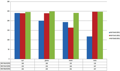
Figure 6. Comparison Graph of Overall Classicification Performance of Four Classifers.

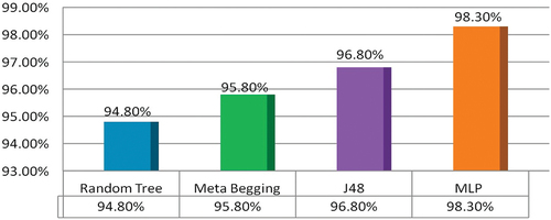
Now we summarize our discussion with the following highlights. This study introduced a novel HBTC framework based on machine vision approaches to classify brain tumors. We successfully designed, implemented, and evaluated all the components of the proposed HBTC framework. In the initial phase, we acquired MR images of four brain tumor types, and after preprocessing, we applied segmentation. Next, we mounted hybrid optimization on the multi-features dataset. Three separate experiments were performed on the ROIs datasets. All the classifiers performed well, but MLP outperformed. Results were not best on a dataset of 10 × 10, as MLP gave maximum accuracy of 64.8% accuracy. Since ROIs were too small, a smaller region did not provide enough information for analysis. Results on the dataset of 15 × 15 were improved, and J48 gave 89.5% accuracy. But results were remarkable on a dataset of 20 × 20, and MLP gave 98.3% accuracy. Compared with others, RT performed less (94.8%) because RT models do not tune the dataset and generate large trees (Kevin Zhou, Fichtinger, and Rueckert 2019). MB showed a better result of 95.8% as it reduces variance and uses a strong aggregate prediction scheme, but still, it does not grasp dataset bias properly (Aslam et al. 2020; Witten 2017). Since J48 applies pruning on the target dataset, non-critical sections of the generated tree are removed, and the over-fitting problem is overcome (Zhou, Rueckert, Daniel,, Fichtinger, Gabor,, 2020). For this reason, J48 produced an average performance of 96.8%. Finally, MLP outmatched others because it provides a strong neural network train-test layered model. It also yields non-linear activations and outperforms on datasets that are linearly non-separable (Asha Kiranmai and Jaya Laxmi 2018; Gonzalez and Rafael 2018; Mohan and Subashini 2018).

It is concluded that the proposed HBTC framework outperformed in the brain tumors classification. A comparison between our proposed framework and other streamed classification techniques is given in Table 11.

Table 11. Comparison of HBTC framework with other streamed classification techniques

Source Citation	Key Features Extracted	Classification	Overall Acc
(Mudda, Manjunath, and Krishnamurthy 2020a)	MRI brain, GLRLM, CSLBP,	ANN	94%
(Seere and Karibasappa 2020)	MRI brain, Homogeneity, Shape, Color, Size, Energy, Contrast	SVM	85.32%
(Ortiz-Ramón et al. 2020)	MRI brain, GLCM, GLRLM, GSSZM NGTDM, LBP.	Linear SVM	89.6%
(Gupta and Sasidhar 2020)	MRI brain, SFTA based texture features	SVM	87%
(Zacharaki et al. 2009)	MRI brain, Statistical & Shape Based, Intensity based, Gabor.	KNN, SVM	90.6%
(Ullah, Batool, and Gilanie 2018)	RD-BVH Brain MRI, Intensity, shape, Texture Features	SVM	97%
(Selvaraj et al. 2007)	MRI brain, Statistical, GLCM	SVM, MPL,	77 to 98%
(Gilanie et al. 2019)	RD-BVH Brain MRI, Texture Features	ANN	86% to 92%
(Tiwari et al. 2017)	MRI brain, Textural Features, GLCM, GLRLM, Gabor, LTEM, FOS	ANN	92.43%
(George and Manuel 2019)	MRI brain, Histogram, First order statistics, GLCM	DNN	91.92%
(Mohsen et al. 2018)	MRI brain, DWT, PCA,	DNN	96.97%
(Bhanumathi and Sangeetha 2019)	MRI brain, Shape, Intensity, Color, Statistics	CNN	97.10%
(Gumaei et al. 2019)	MRI brain, Gabor, GWT, GIST-descriptor, N-GIST (normalized)	RELM	94.233%
Proposed Methodology	HBTC framework	MLP	98.3%

Conclusion

The main objective of this research study was to classify four brain tumor types using a novel machine vision-based HBTC framework. The proposed framework input MRIs and applied histogram equalization to normalize brain images, and the hybrid K-S-L scheme reduced the image noise. To segment the tumor region, we carried out the TACS scheme. Following that multiple feature extraction approaches were used to extract texture characteristics of brain tumors. The multi-features dataset included COM, RLM, and Gradient texture features. Next, our framework applied a hybrid multi-features optimization method on the feature vector, which produced a fully optimized feature dataset. In the end, MV classifiers, namely RT, MB, J48, and MLP, were evaluated on the dataset. All classifiers provide splendid results, but MLP showed outstanding accuracy of 98.3% to classify four brain tumors. The average accuracy of J48, MB, and RT was 96.8%, 95.8%, and 94.8%, respectively. The framework will help radiologists and doctors to diagnose brain tumors correctly. The framework is robust and will surely minimize human error in diagnosing brain tumors.

Future Work

In the future, this study will be performed using different modalities and other brain tumor types.

Data Availability

The dataset will be provided on demand for research study.

Acknowledgments

This work was supported by IUB and MNS-UAM. The authors would like to thank Dr. Kamran (RD-BVH), Mr. Tanveer Aslam, Mr. Umer (RD-BVH) for technical and field assistance.

Disclosure statement

No potential conflict of interest was reported by the author(s).

Additional information

Funding

This Research did not receive any specific grant from any public, commercial or non-profit able funding agencies.

References

- Al-Kilidar, S. H. S., and L. E. George. 2020. Texture Classification Using Gradient Features with Artificial Neural Network. Journal of Southwest Jiaotong University 55 (1):1–1977. doi:10.35741/.0258-2724.55.1.13.
- Alfonse, M., and A.-B. M. Salem . 2016. An Automatic Classification of Brain Tumors through MRI Using Support Vector Machine. Egyptian Computer Science Journal 40 (3): 11–21. http://ecsjournal.org/Archive/Volume40/Issue3/2.pdf .
- Anter, A. M., and A. Ella Hassenian. 2018. Normalized Multiple Features Fusion Based on PCA and Multiple Classifiers Voting in CT Liver Tumor Recognition. Studies in Computational Intelligence 730 (May):113–29. doi:10.1007/978-3-319-63754-9_6.
- Arunkumar, N., M. A. Abed Mohammed, S. A. Mostafa, D. A. Ahmed Ibrahim, J. J. P. C. Rodrigues, and V. H. C. de Albuquerque. 2020. Fully Automatic Model-Based Segmentation and Classification Approach for MRI Brain Tumor Using Artificial Neural Networks. Concurrency and Computation: Practice and Experience 32 (1):1–9. doi:10.1002/cpe.4962.
- Asha Kiranmai, S., and A. Jaya Laxmi. 2018. Data Mining for Classification of Power Quality Problems Using WEKA and the Effect of Attributes on Classification Accuracy. Protection and Control of Modern Power Systems 3 (1):1–12. doi:10.1186/s41601-018-0103-3.
- Aslam, T., S. Qadri, M. Shehzad, S. Furqan Qadri, A. Razzaq, and S. Shah. 2020. Emotion Based Facial Expression Detection Using Machine Learning. Life Science Journal 17 (8):35–43. http://www.lifesciencesite.com/lsj/lsj170820/06_36691lsj170820_35_43.pdf.
- Attique, M., G. Gilanie, H.-U. Hafeez-Ullah, M. S. Mehmood, M. S. Naweed, M. Ikram, J. A. Kamran, and A. Vitkin. 2012. Colorization and Automated Segmentation of Human T2 MR Brain Images for Characterization of Soft Tissues. PLoS ONE 7 (3):1–13. doi:10.1371/journal.pone.0033616.
- Baessler, B., T. Nestler, D. P. Dos Santos, P. Paffenholz, V. Zeuch, D. Pfister, D. Maintz, and A. Heidenreich. 2020. Radiomics Allows for Detection of Benign and Malignant Histopathology in Patients with Metastatic Testicular Germ Cell Tumors Prior to Post-Chemotherapy Retroperitoneal Lymph Node Dissection. European Radiology 30 (4):2334–45. doi:10.1007/s00330-019-06495-z.
- Batchelor, B. G. 2012a. Machine Vision for Industrial Applications. In Machine Vision Handbook, ed. B. G. Batchelor, 2nd ed., 2012. 1–59. London: Springer-Verlag London Limited.
- Batchelor, B. G, Whelan, Paul F. 2012. Basic Machine Vision Techniques. In Machine Vision Handbook, ed. B. G. Batchelor, 2nd 2 London: Springer-Verlag London Limited 565–623. 10.1007/978-1-84996-169-1
- Batchelor, B. G., and P. F. Whelan. 2012. Basic Machine Vision Techniques. Machine Vision Handbook. doi:10.1007/978-1-84996-169-1_14.
- Bhanumathi, V., and R. Sangeetha. 2019. “CNN Based Training and Classification of MRI Brain Images.” In 2019 5th International Conference on Advanced Computing and Communication Systems, ICACCS 2019 15-16 March 2019 (IEEE) Coimbatore, India, 129–33. doi: 10.1109/ICACCS.2019.8728447.
- Bianconi, E., A. Piovesan, F. Facchin, A. Beraudi, R. Casadei, F. Frabetti, L. Vitale, M. C. Pelleri, S. Tassani, F. Piva, et al. 2013. An Estimation of the Number of Cells in the Human Body. Annals of Human Biology 40 (6):463–71. doi:10.3109/03014460.2013.807878.
- Bloom, D. E., and D. Cadarette. 2019. Infectious Disease Threats in the Twenty-First Century: Strengthening the Global Response. Frontiers in Immunology 10 (MAR):1–12. doi:10.3389/fimmu.2019.00549.
- Chandrashekar, G., and F. Sahin. 2014. A Survey on Feature Selection Methods. Computers & Electrical Engineering 40 (1):16–28. doi:10.1016/j.compeleceng.2013.11.024.
- Chourmouzi, D., E. Papadopoulou, K. Marias, and A. Drevelegas. 2014. Imaging of Brain Tumors. Surgical Oncology Clinics of North America 23 (4):629–84. doi:10.1016/j.soc.2014.07.004.
- Dilliraj, E., P. Vadivu, and A. Anbarasi. 2014. MR Brain Image Segmentation Based on Self- Organizing Map and Neural Network. International Journal for Research in Applied Science & Engineering Technology (IJRASET). 2 (Xii):524–29.
- El-Dahshan, E. A. S., H. M. Mohsen, K. Revett, and A. B. M. Salem. 2014. Computer-Aided Diagnosis of Human Brain Tumor through MRI: A Survey and a New Algorithm. Expert Systems with Applications 41 (11):5526–45. doi:10.1016/j.eswa.2014.01.021.
- Ferlay, J., M. Colombet, I. Soerjomataram, D. M. Parkin, M. Piñeros, A. Znaor, and F. Bray. 2021. Cancer Statistics for the Year 2020: An Overview. International Journal of Cancer 149 (4):778–89. doi:10.1002/ijc.33588.
- George, N., and M. Manuel. 2019. “A Four Grade Brain Tumor Classification System Using Deep Neural Network.” In 2019 2nd International Conference on Signal Processing and Communication (ICSPC), Coimbatore, INDIA (IEEE), 127–32. doi: 10.1109/ICSPC46172.2019.8976495.
- Gilanie, G., U. I. Ijaz Bajwa, M. M. Mahmood Waraich, and Z. Habib. 2019. Automated and Reliable Brain Radiology with Texture Analysis of Magnetic Resonance Imaging and Cross Datasets Validation. International Journal of Imaging Systems and Technology 29 (4):531–38. doi:10.1002/ima.22333.
- Gonzalez, R. E. W., and C. Rafael. 2018. Digital Image Processing, 4th Pearson 2018. Edited by 4. Pearson. New York: Pearson. ISBN: 13: 9780133356724 . https://www.pearson.com/us/higher-education/program/Gonzalez-Digital-Image-Processing-4th-Edition/PGM241219.html
- Gumaei, A., M. M. Mehedi Hassan, M. R. Rafiul Hassan, A. Alelaiwi, and G. Fortino. 2019. A Hybrid Feature Extraction Method with Regularized Extreme Learning Machine for Brain Tumor Classification. IEEE Access 7:36266–73. doi:10.1109/ACCESS.2019.2904145.
- Gupta, M., and K. Sasidhar. 2020. “Non-Invasive Brain Tumor Detection Using Magnetic Resonance Imaging Based Fractal Texture Features and Shape Measures.” Proceedings of 3rd International Conference on Emerging Technologies in Computer Engineering: Machine Learning and Internet of Things, ICETCE 2020 Jaipur, India (IEEE), 93–97. doi: 10.1109/ICETCE48199.2020.9091756.
- Hajian-Tilaki, K. 2013. Receiver Operating Characteristic (ROC) Curve Analysis for Medical Diagnostic Test Evaluation. Caspian Journal of Internal Medicine 4 (2):627–35.
- Haralick, R. M., K. Shanmugam, and I. Dinstein. 1973. Textural Features for Image Classification. IEEE Transactions on Systems, Man, and Cybernetics SMC-3 (6):610–21. doi:10.1109/TSMC.1973.4309314.
- Heba, M., E. Sayed Ahmed El-Dahshan, and A. B. M. Salem. 2012. “A Machine Learning Technique for MRI Brain Images.” 2012 8th International Conference on Informatics and Systems, INFOS 2012 Giza, Egypt (IEEE)BIO-161-BIO-165 , no. January.
- Husham, S., A. Mustapha, S. A. Mostafa, M. K. Al-Obaidi, M. Abed Mohammed, A. Idrees Abdulmaged, and S. Thomas George. 2021. Comparative Analysis between Active Contour and Otsu Thresholding Segmentation Algorithms in Segmenting Brain Tumor Magnetic Resonance Imaging. Journal of Information Technology Management 12:48–61. doi:10.22059/JITM.2020.78889.
- Iqbal, J., Dr 2009. “Bahawal Victoria Hospital.” 2009. https://www.flickr.com/photos/ammarkh/3804464335/.
- Kevin Zhou, S., G. Fichtinger, and D. Rueckert. 2019. Random forests in medical image computing. In Handbook of Medical Image Computing and Computer Assisted Intervention , 457–80. London, UK: ELESVIER Academic Press. doi:10.1016/C2017-0-04608-6.
- Lakshmi Devasena, C., and M. Hemalatha. 2011. Noise Removal in Magnetic Resonance Images Using Hybrid KSL Filtering Technique. International Journal of Computer Applications 27 (8):1–4. doi:10.5120/3324-4571.
- Louis, D. N., A. Perry, G. Reifenberger, A. von Deimling, D. Figarella-Branger, W. K. Cavenee, H. Ohgaki, O. D. Wiestler, P. Kleihues, and D. W. Ellison. 2016. The 2016 World Health Organization Classification of Tumors of the Central Nervous System: A Summary. Acta Neuropathologica 131 (6):803–20. http://link.springer.de/link/service/journals/00401/index.htm%5Cnhttp://ovidsp.ovid.com/ovidweb.cgi?T=JS&PAGE=reference&D=emed18a&NEWS=N&AN=610343744.
- Mohammed, M. A., B. Al-Khateeb, A. N. Noori Rashid, D. A. Ahmed Ibrahim, M. K. Khanapi Abd Ghani, and S. A. Mostafa. 2018. Neural Network and Multi-Fractal Dimension Features for Breast Cancer Classification from Ultrasound Images. Computers & Electrical Engineering 70:871–82. doi:10.1016/j.compeleceng.2018.01.033.
- Mohan, G., and M. Monica Subashini. 2018. MRI Based Medical Image Analysis: Survey on Brain Tumor Grade Classification. Biomedical Signal Processing and Control 39:139–61. doi:10.1016/j.bspc.2017.07.007.
- Mohsen, H., E. S. A. El-Dahshan, E. S. M. El-Horbaty, and A. B. M. Salem. 2018. Classification Using Deep Learning Neural Networks for Brain Tumors. Future Computing and Informatics Journal 3 (1):68–71. doi:10.1016/j.fcij.2017.12.001.
- Mostafa, S. A., A. Mustapha, M. A. Abed Mohammed, R. I. Raed Ibraheem Hamed, N. Arunkumar, M. K. Abd Ghani, M. M. Jaber, and S. H. Khaleefah. 2019. Examining Multiple Feature Evaluation and Classification Methods for Improving the Diagnosis of Parkinson’s Disease. Cognitive Systems Research 54 :90–99. doi:10.1016/j.cogsys.2018.12.004.
- Mudda, M., R. Manjunath, and N. Krishnamurthy. 2020a. Brain Tumor Classification Using Enhanced Statistical Texture Features. IETE Journal of Research 1–12. doi:10.1080/03772063.2020.1775501.
- Ortiz-Ramón, R., S. Ruiz-España, E. Mollá-Olmos, and D. Moratal. 2020. Glioblastomas and Brain Metastases Differentiation Following an MRI Texture Analysis-Based Radiomics Approach. Physica Medica 76:44–54. doi:10.1016/j.ejmp.2020.06.016.
- Patel, K. K., S. M. Patel, and P. G. Scholar. 2016. Internet of Things-IOT: Definition, Characteristics, Architecture, Enabling Technologies, Application & Future Challenges. International Journal of Engineering Science and Computing 6 (5):1–10. doi:10.4010/2016.1482.
- Pereira, S., A. Pinto, V. Alves, and C. A. Silva. 2016. Brain Tumor Segmentation Using Convolutional Neural Networks in MRI Images. IEEE Transactions on Medical Imaging 35 (5):1240–51. doi:10.1109/TMI.2016.2538465.
- Perkins, A., and G. Liu. 2016. Primary Brain Tumors in Adults: Diagnosis and Treatment - American Family Physician. American Family Physician 93 (3):211–18. www.aafp.org/afp.
- Phal, P. M., A. Usmanov, G. M. Nesbit, J. C. Anderson, D. Spencer, P. Wang, J. A. Helwig, C. Roberts, and B. E. Hamilton. 2008. Qualitative Comparison of 3-T and 1.5-T MRI in the Evaluation of Epilepsy. American Journal of Roentgenology 191 (3):890–95. doi:10.2214/AJR.07.3933.
- Qadri, S., S. Furqan Qadri, M. Husnain, M. M. Muhammad Saad Missen, D. M. Muhammad Khan, Muzammil-Ul-Rehman, A. Razzaq, and S. Ullah. 2019. Machine Vision Approach for Classification of Citrus Leaves Using Fused Features. International Journal of Food Properties 22 (1):2071–88. doi:10.1080/10942912.2019.1703738.
- Radhakrishnan, M., and T. Kuttiannan. 2012. Comparative Analysis of Feature Extraction Methods for the Classification of Prostate Cancer from TRUS Medical Images. International Journal of Computer Science Issues 9 (1):171–79.
- Sachdeva, J., V. Kumar, I. Gupta, N. Khandelwal, and C. K. Kamal Ahuja. 2013. Segmentation, Feature Extraction, and Multiclass Brain Tumor Classification. Journal of Digital Imaging 26 (6):1141–50. doi:10.1007/s10278-013-9600-0.
- Saqlain, S. M., M. Sher, F. A. Ali Shah, I. Khan, M. U. Usman Ashraf, M. Awais, and A. Ghani. 2019. Fisher Score and Matthews Correlation Coefficient-Based Feature Subset Selection for Heart Disease Diagnosis Using Support Vector Machines. Knowledge and Information Systems 58 (1):139–67. doi:10.1007/s10115-018-1185-y.
- Seere, S. K., and K. Karibasappa. 2020. Threshold Segmentation and Watershed Segmentation Algorithm for Brain Tumor Detection Using Support Vector Machine. European Journal of Engineering Research and Science 5 (4):516–19. doi:10.24018/ejers.2020.5.4.1902.
- Selvaraj, H., S. Thamarai Selvi, D. Selvathi, and L. Gewali. 2007. Brain Mri Slices Classification Using Least Squares Support Vector Machine. IC-MED International Journal of Intelligent Computing in Medical Sciences and Image Processing 1 (1):21–33. doi:10.1080/1931308X.2007.10644134.
- Shehzad, M., S. Qadri, T. Aslam, S. Furqan Qadri, A. Razzaq, S. Shah Muhammad, S. Ali Nawaz, and N. Ahmad. 2020. Machine Vision Based Identification of Eye Cataract Stages Using Texture Features. Life Science Journal 17 (8):44–50. doi:10.7537/marslsj170820.07.
- Sinha, T. 2018. Tumors: Benign and Malignant. Cancer Therapy & Oncology International Journal 10 (3):1–3. doi:10.19080/ctoij.2018.10.555790.
- Strong, M. J., J. Garces, J. C. Vera, M. Mathkour, N. Emerson, and M. L. Ware. 2016. Brain Tumors: Epidemiology and Current Trends in Treatment. Journal of Brain Tumors & Neurooncology 1 (1):1–21. doi:10.4172/2475-3203.1000102.
- Strzelecki, M., P. Szczypinski, A. Materka, and A. Klepaczko. 2013. A Software Tool for Automatic Classification and Segmentation of 2D/3D Medical Images. Nuclear Instruments & Methods in Physics Research. Section A, Accelerators, Spectrometers, Detectors and Associated Equipment 702:137–40. doi:10.1016/j.nima.2012.09.006.
- Sung, H., J. Ferlay, R. L. Siegel, M. Laversanne, I. Soerjomataram, A. Jemal, and F. Bray. 2021. Global Cancer Statistics 2020: GLOBOCAN Estimates of Incidence and Mortality Worldwide for 36 Cancers in 185 Countries. CA: A Cancer Journal for Clinicians 71 (3):209–49. doi:10.3322/caac.21660.
- Tiwari, P., J. Sachdeva, C. K. Kamal Ahuja, and N. Khandelwal. 2017. Computer Aided Diagnosis System-A Decision Support System for Clinical Diagnosis of Brain Tumours. International Journal of Computational Intelligence Systems 10 (1):104–19. doi:10.2991/ijcis.2017.10.1.8.
- Ullah, H., A. Batool, and G. Gilanie. 2018. Classification of Brain Tumor with Statistical Analysis of Texture Parameter Using a Data Mining Technique. International Journal of Industrial Biotechnology and Biomaterials 4 (2): 22–36 . February 2019.
- von Bartheld, C. S., J. Bahney, and S. Herculano-Houzel. 2016. The Search for True Numbers of Neurons and Glial Cells in the Human Brain: A Review of 150 Years of Cell Counting. Journal of Comparative Neurology 524 (18):3865–95. doi:10.1002/cne.24040.
- Wahid, F., M. Fayaz, and A. S. Salam Shah. 2016. An Evaluation of Automated Tumor Detection Techniques of Brain Magnetic Resonance Imaging (MRI). International Journal of Bio-Science and Bio-Technology 8 (2):265–78. doi:10.14257/ijbsbt.2016.8.2.25.
- Witten, I. H., E. Frank, M. A. Hall, and C. J. Pal. 2016. The Weka Workbench. In Data Mining: Practical Machine Learning Tools and Techniques, Fourth ed., 1–128. Cambridge, MA , United States: Morgan Kaufmann. https://www.cs.waikato.ac.nz/ml/weka/Witten_et_al_2016_appendix.pdf.
- Witten, I. H, Frank, Eibe, Hall, Mark A., Pal, Christopher J. 2017. Data Mining Practical Machine Learning Tools and Techniques. Fourth Edition) ed. Cambridge, MA , United States: Morgan Kaufmann. ISBN: 978-0-12-804291-5 .
- Zacharaki, E. I., S. Wang, S. Chawla, D. Soo Yoo, R. Wolf, E. R. Melhem, and C. Davatzikos. 2009. Classification of Brain Tumor Type and Grade Using MRI Texture and Shape in a Machine Learning Scheme. Magnetic Resonance in Medicine 62 (6):1609–18. doi:10.1002/mrm.22147.
- Zhao, J., Z. Meng, L. Wei, C. Sun, Q. Zou, and R. Su. 2019. Supervised Brain Tumor Segmentation Based on Gradient and Context-Sensitive Features. Frontiers in Neuroscience 13 (44):1–11. doi:10.3389/fnins.2019.00144.
- Zhou, S. K., D. Rueckert, and G. Fichtinger. 2020. Handbook of Medical Image Computing and Computer Assisted Intervention. London, United Kingdom: Academic Press.