A Bayesian Allocation Model Based Approach to Mixed Membership Stochastic Blockmodels

ABSTRACT

Although detecting communities in networks has attracted considerable recent attention, estimating the number of communities is still an open problem. In this paper, we propose a model, which replicates the generative process of the mixed-membership stochastic block model (MMSB) within the generic allocation framework of Bayesian allocation model (BAM) and BAM-MMSB. In contrast to traditional blockmodels, BAM-MMSB considers the observations as Poisson counts generated by a base Poisson process and marks according to the generative process of MMSB. Moreover, the optimal number of communities for BAM-MMSB is estimated by computing the variational approximations of the marginal likelihood for each model order. Experiments on synthetic and real data sets show that the proposed approach promises a generalized model selection solution that can choose not only the model size but also the most appropriate decomposition.

Introduction

Complex interaction structures among individual components are commonly represented using networks or graphs. They provide a mathematical framework to study relational data sets to define relations such as human interactions in sociometry, protein–protein interactions in biology, and computer interactions in information technology. As relational data sets have grown tremendously, the need to understand and interpret the properties of large, complex networks has emerged. Network analysis aims to discover latent structures in large relational data sets in order to determine elements with similar properties based on the observed and modeled relationships (Goldenberg et al. 2010). A fundamental tool for discovering latent structures in large relational data sets is to decompose a complex network into its building blocks called communities (Peixoto 2017). In order to find the communities in complex networks, several methods have been proposed. Methods that optimize the cost function of a given metric, such as modularity (Newman 2006b) suffer from being only heuristically motivated (Gerlach, Peixoto, and Altmann 2018). Probabilistic generative models provide rigorous methods for model selection based on statistical evidence (Riolo et al. 2017).

Compared to the amount of work on community detection, there is little work on the model selection problem, which corresponds to selecting the optimal number of communities. Generative models provide principled likelihood-based approaches exploiting Bayesian model selection procedures. Recent studies in the literature are based on estimation of the marginal likelihood using variational approximations (Fosdick et al. 2019; Latouche, Birmele, and Ambroise 2012), Bayesian Information Criterion-based approximations (Peixoto 2015), spectral models (Le and Levina 2019) and non-parametric methods (Geng, Bhattacharya, and Pati 2019; Riolo et al. 2017).

For relational data, one of the most popular generative models is the stochastic blockmodel (SBM) (Holland, Blackmond Laskey, and Leinhardt 1983; Newman and Reinert 2016). It is a random graph model that defines a mixture of Bernoullis over relational data. Its generative process assigns each node $i$ to a block $z_i$ and accordingly, the edges are drawn independently conditioned on their block memberships. For each node pair $\{i,j\}$, the probability of an edge $\{i,j\}$ is equal to ${\mathbf{B}}_{z_i,z_j}$ where $\mathbf{B}$ is a $K\times K$ block matrix containing the connection probabilities of $K$ blocks.

The generative process of SBM produces non-overlapping communities with homogeneous Poisson degree distributions within the blocks under the assumption that a single object belongs to a single community. In real-world networks, objects generally belong to several communities. Some extensions of SBMs, such as overlapping (Latouche, Birmele, and Ambroise et al. 2011), mixed membership stochastic blockmodel (MMSB) (Airoldi et al. 2008) and degree corrected SBMs (Brian and Newman 2011) have been proposed to address overlapping structures in networks. Among these, MMSB is a mixed-membership model similar to Latent Dirichlet Allocation (LDA) (Blei, Ng, and Jordan 2003) but defined for relational data. The generative process of MMSB associates each node with multiple blocks through a membership vector, which allows for non-overlapping communities.

Many distinct generative models have been proposed for relational data in different contexts such as LDA (Blei, Ng, and Jordan 2003), Principal Component Analysis (W. Buntine 2002), and factor model (Canny 2004). Although they are different models, their relevance to each other is explained in (Buntine, Wray, and Jakulin 2006; Cemgil et al. 2019) In this regard, the Bayesian allocation model (BAM) (Cemgil et al. 2019) proposes a dynamical model that is able to replicate other discrete generative processes within a generic allocation framework. In particular, BAM allocates the observations to latent variables that respect a given factorization implied by a domain-specific directed graphical model $\mathcal{G}=(\mathcal{V},\mathcal{E})$, where $\mathcal{V}$ and $\mathcal{E}$ denote the nodes and the edges, respectively.

In this paper, we propose to model mixed-membership stochastic blockmodels as an instance of BAM. This choice is motivated by the fact that BAM provides a generic allocation framework for discrete observations (Hızlı, Taylan Cemgil, and Kırbız 2019). Furthermore, BAM allows for a principled Bayesian model selection procedure. Although we only perform model order selection in this paper, we believe that the generic allocation perspective of BAM promises a generalized model selection solution where we can both select the model order and choose the best factorization. Moreover, the variational inference algorithm is also extended to handle the missing data problem.

The rest of the paper is organized as follows. In Section 2, we review the modeling elements for text and graphs. In Section 3, the proposed model is described in detail. Section 4 represents the inference algorithms. Section 5 displays the model selection performance of the proposed algorithm compared to MMSB both under synthetic and benchmark networks. Finally, we conclude the paper and give some future work.

Background Information

In this section, we will give a brief description of probabilistic generative models, such as Stochastic Blockmodel, Mixed-Membership Stochastic Blockmodel and Bayesian Allocation Model, which give the building motivation for the proposed method.

Stochastic Blockmodel

SBM is a mixture model defined for relational data. We assume that the vertices $V$ of a graph $G=(V,E)$ are clustered into $K$ blocks and try to find the $K$ blocks of a network consisting of similar nodes in terms of their connectivity patterns. For a graph with $N$ nodes, $K$ blocks, and the adjacency matrix $Y\in \{0,1{\}}^{N\times N}$, the connectivity pattern $C_i$ of node $i$ can be formalized as (Goldenberg et al. 2010): $C_i\equiv \{Y(i,j\in k):\mathrm{\forall }k\in [K]\},$ where $j\in k$ iterates over each node in block $k$. The connectivity pattern $C_i$ represents how node $i$ connects to the nodes belonging to each $k\in [K]\equiv \{1,\cdots ,K\}$ given the nodes and their corresponding blocks. If nodes $i$ and $r$ connect to the same set of nodes with similar probabilistic measures, $C_i\approx C_r$, they are stochastically equivalent (Holland, Blackmond Laskey, and Leinhardt 1983).

The generative process of SBM produces stochastically equivalent nodes within the categories they belong to. The updated generative process is described as follows:

(1) For each block pair $(k,l)\in K\times K$:

(a) Choose interaction probability, $B_{kl}\sim \mathcal{B}(a_{kl},b_{kl})$.

(2) Choose block proportions, $\pi \sim \mathcal{D}(\alpha )$, where $\pi ,\alpha \in {\mathbb{R}}^K$

(3) For each node $i\in V$:

i. Choose block membership, $z_i\sim \mathcal{M}(\pi )$.

(4) For each node pair $(i,j)\in N\times N$: [i.]

i. Choose interaction, $Y_{ij}\sim \mathcal{B}\mathcal{E}(B_{z_i{z}_j})$.

In this process, $\mathcal{B},\mathcal{D},\mathcal{M},\mathcal{B}\mathcal{E}$ correspond to Beta, Dirichlet, Multinomial, and Bernoulli distributions, respectively. The joint probability distribution is obtained as:

(1) $p(Y,B,Z,\pi )=p(\pi |\alpha )\times \prod _{kl}p(B_{kl}|a_{kl},b_{kl})\times \prod _{i}p(z_i|\pi )\times \prod _{ij}p(Y_{ij}|B_{z_i{z}_j}).$(1)

In real-world networks, blocks or communities are not mutually exclusive. Since SBMs follow a hard clustering methodology by assigning each node as a member of one block strictly, SBMs are unable to model this.

Mixed-Membership Stochastic Blockmodel

A possible extension to SBM is proposed for overlapping communities: MMSB (Airoldi et al. 2008). MMSB considers each membership vector ${\theta }_i\in {\mathbb{R}}^K$ of node $i$ as a Dirichlet distribution, i.e., a point on $K-1$ simplex. Each point on $K-1$ simplex represents $K$ non-negative weights whose sum is equal to $1$. The MMSB offers a realistic type of soft clustering using the following generative process:

(1) For each block pair $(k,l)\in K\times K$:

(a) Choose interaction probability, $B_{kl}\sim \mathcal{B}(a_{kl},b_{kl})$.

(2) For each node $i\in V$:

(a) Choose a mixed membership vector, ${\pi }_i\sim \mathcal{D}({\alpha }_K)$.

(3) For each node pair $(i,j)\in N\times N$:

(a) Choose membership for source, $z_{i\to j}\sim \mathcal{M}({\pi }_i)$.

(b) Choose membership for destination, $z_{i\leftarrow j}\sim \mathcal{M}({\vec{\pi }}_j)$.

(c) Choose interaction, $Y_{ij}\sim \mathcal{B}\mathcal{E}(z_{i\to j}^{T}B{z}_{i\leftarrow j})$.

The main difference between MMSB and SBM is that $z_i$ and $z_j$ vectors of MMSB are not one-of-$N$ vectors but are probability distributions and the sum of their elements is equal to one. Then, the joint probability becomes:

$p(Y,Z,B,\pi )=\prod _{kl}p(B_{kl}|a_{kl},b_{kl})\prod _{i}p({\pi }_i|\alpha )\prod _{ij}p({\vec{z}}_{i\to j}|{\pi }_i)p({\vec{z}}_{i\leftarrow j}|{\pi }_j)p(Y_{ij}|{\vec{z}}_{i\to j}^{T}B{\vec{z}}_{i\leftarrow j}).$

Another feature of MMSB is that it is built as a mixed-membership model, which has a close relation with the generalized allocation scheme of BAM. From the generalization perspective, although it is possible to infer the latent variables directly from the generative process above, we choose to model MMSB as an instance of BAM. In this way, we aim to exploit the flexible framework of BAM.

Bayesian Allocation Model

BAM builds up a generic generative model framework for discrete count data. It is composed of two processes:

(1) Generation: It defines a base Poisson process, which is expected to generate $T$ number of tokens equal to the total number of observations at timestamps $0<t_1,t_2,\dots ,t_T<1$.

(2) Allocation: At each timestamp, each token is marked as a member of a specific Poisson process indexed by $i_{1:N}$ where each index $i_n$ represents a discrete random variable with $I_n$ many states. Then, the index collection $i_{1:N}$ represents the set of all possible indices for ${\prod }_n{I}_n$ possible values of state combinations.

Allocation process produces ${\prod }_n{I}_n$ different Poisson processes, which can be viewed as indices of an allocation tensor, $S$. Hence, it is insightful to think of each process $S(i_{1:N})$ as a box, each generated token at timestamp $\tau$ as balls and allocation tensor $S$ as the collection of boxes filled with balls. The allocation process during the lifespan of $S$ can be summarized as follows: [$\circ$]

° $S$ is empty at $t=0$.

° Base process generates $T$ balls with the timestamps $0<t_1,t_2,\dots ,t_T<1$.

° Each ball is marked to an index of $S(i_{1:N})$ with probability $\theta (i_{1:N})$ independently.

° Each joint probability $\theta (i_{1:N})$ can be factorized into conditional probability tables (CPT) implied by the given Bayesian network $\mathcal{G}$ of the domain-specific model.

° At $t=T$, the total of $T$ balls is marked and allocated to the allocation tensor $S$.

The joint distribution of the assignments becomes a high-dimensional array for discrete models where $i_{1:N}$ corresponds to the likeliness of a specific configuration. The probability tensor $\theta \in {\mathbb{R}}^N$ obeys a given factorization implied by a Bayesian network $\mathcal{G}$, representing conditional dependence assumptions of the domain-specific model. In box analogy, each entry ${\theta }_{i_{1:N}}$ tells us how likely it is for a ball to be marked with color $i_{1:N}$ and placed into the box $i_{1:N}$. Based on the factorization implied by $\mathcal{G}$, the probability of a ball being marked with the color $i_{1:N}$ is:

(2) $\theta (i_{1:N})=\prod _n{\theta }_{n|pa(n)}(i_n,i_{pa(n)})$(2)

where $i_{pa(n)}$ are the parent nodes of $i_n$. The hyperparameter $\alpha$ for the probability tensor $\theta$ contains Dirichlet measures with entries $\alpha (i_{1:N})$. Furthermore, it is important to keep the measures of each Dirichlet random variable consistent (Cemgil et al. 2019). To impose structural constraints consistently on implied factorizations, the following contractions are needed:

${\alpha }_{n|pa(n)}(i_n,i_{pa(n)})=\sum _{i_{\mathrm{\neg }fa(n)}}\alpha (i_{1:N})$

where $i_{\mathrm{\neg }fa(n)}$ are the nodes, which are not in the family of $i_n$ and ${\alpha }_{n|pa(n)}(i_n,i_{pa(n)})$ represents Dirichlet measures for the Dirichlet random variable ${\theta }_{n|pa(n)}(i_n,i_{pa(n)})$:

${\theta }_{n|pa(n)}(:,i_{pa(n)})\sim \mathcal{D}({\alpha }_{n|pa(n)}(:,i_{pa(n)}))$

Then, we can summarize the generative process of BAM as follows;

$\lambda \sim \mathcal{G}\mathcal{A}(a,b){\theta }_{n|pa(n)}(:,i_{pa(n)})\sim \mathcal{D}({\alpha }_{n|pa(n)}(:,i_{pa(n)}))$

$S(i_{1:N})\sim \mathcal{P}\mathcal{O}(\lambda \prod _{n=1}^N{\theta }_{n|pa(n)}(:,i_{pa(n)}))X(i_V)=\sum _{i_{\bar{V}}}S(i_{1:N})$

where $i_V$ and $i_{\bar{V}}$ denote for the observed and the latent index set, respectively. A natural choice for $⟨\lambda ⟩=a/b$ is the expected number of tokens observed until time $t=1$. By defining $S_{+}={\sum }_{i_{1:N}}{S}_{i_{1:N}}$, the scale parameter can be chosen $b\sim a/S_{+}$ (Cemgil et al. 2019).

MMSB as an Instance of BAM

MMSB is a hierarchical latent model defined on discrete network data that can be realized through BAM. This is due to the fact that BAM provides a generic allocation framework for discrete observations. In particular, BAM allows for allocating discrete observations to latent classes with respect to any given factorization implied by a directed graphical model $\mathcal{G}$. Thanks to its inherent flexibility, BAM promises a generalized solution where we not only select the model order but also choose the most appropriate model for a given empirical network.

To be able to see the relation, let us define the following indicators to encode events for token $\tau \in [S_{+}]$ where $S_{+}$ is the total number of tokens and $[S_{+}]\equiv \{1,\cdots ,S_{+}\}$:

• $c_{i\tau }$: token $\tau$ selects source $i$.

• $d_{j\tau }$: token $\tau$ selects destination $j$.

• $z_{k\tau }^{\to }$: token $\tau$ selects source block $k$.

• $z_{l\tau }^{\leftarrow }$: token $\tau$ selects destination block $l$.

• $t_{s\tau }$: token $\tau$ selects interaction $s$;

Similar to the generative process of MMSB described in Section 2.2, we can define a hierarchical Dirichlet-Multinomial model over the indicators. The generative process for the indicators is as follows:

${\gamma }_{:}\sim \mathcal{D}({\eta }_{\gamma }){\varphi }_{:}\sim \mathcal{D}({\eta }_{\varphi })$

$c_{:\tau }\sim \mathcal{M}({\gamma }_{:},1)d_{:\tau }\sim \mathcal{M}({\varphi }_{:},1)$

${\pi }_{:i}\sim \mathcal{D}({\eta }_{{\pi }_i}){\pi }_{:j}\sim \mathcal{D}({\eta }_{{\pi }_j})$

$z_{:\tau }^{\to }|c_{:\tau }\sim \prod _i\mathcal{M}({\pi }_{:i},1{)}^{c_{i\tau }}{z}_{:\tau }^{\leftarrow }|d_{:\tau }\sim \prod _j\mathcal{M}({\pi }_{:j},1{)}^{d_{j\tau }}$

${\beta }_{:kl}\sim \mathcal{D}({\eta }_{\beta })t_{:\tau }|z_{:\tau }^{\to },z_{:\tau }^{\leftarrow }\sim \prod _k\prod _l\mathcal{M}({\beta }_{:kl},1{)}^{z_{k\tau }^{\to }{z}_{l\tau }^{\leftarrow }}$

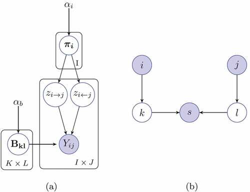
BAM visualizes this sequential index selection through its graphical model notation. Each generated token selects an index set of the form $\{i,k,s,l,j\}$ while the observed index set is $V=\{i,s,j\}$ and latent index set is $\bar{V}=\{k,l\}$. This notation is simpler than the traditional plate representation used to show graphical patterns of indexed data as illustrated in Figure 1. Then, each index of the joint indicator becomes

(3) $s_{ikslj}^{\tau }=c_{i\tau }\wedge z_{k\tau }^{\to }\wedge t_{s\tau }\wedge z_{l\tau }^{\leftarrow }\wedge d_{j\tau },$(3)

Figure 1. Comparison of MMSB graphical models: (a) Traditional (b) Graphical model in BAM notation.

where $\wedge$ is the logical AND operator. This implies that the joint indicator is categorically distributed with $s^{\tau }\sim \mathcal{M}(\theta ,1)$ with each cell having an assignment probability;

${\theta }_{ikslj}={\gamma }_i\cdot {\pi }_{ki}\cdot {\beta }_{skl}\cdot {\pi }_{lj}\cdot {\varphi }_j={\theta }_i\cdot {\theta }_{k|i}\cdot {\theta }_{s|k,l}\cdot {\theta }_{l|j}\cdot {\theta }_j$

Note that, notation ${\theta }_{s|k,l}$ is preferred in place of ${\theta }_{s|k,l}(s,k,l)$ for simplicity. The random variable index $s$ is added to the random variable indices $k,l,i,j$ of MMSB because BAM is defined on Poisson counts in contrast to Bernoulli random variables representing relational data in the generative model of MMSB. The added index $s$ allows for an equivalent representation in the form of count data when the sum ${\sum }_s{S}_{ikslj}$ of each $S_{ik:lj}$ fiber is constrained to 1. This setup is described in detail in Section 5.

Continuing with the generative process of BAM, each index of the allocation tensor $S$ is defined as the collection of all tokens occurring at times $\tau :S_{ikslj}={\sum }_{\tau }{s}_{ikslj}^{\tau }$. Accordingly, conditioned on the sum $S_{+}={\sum }_{ikslj}{\sum }_{\tau }{s}_{iksjl}^{\tau }$, the allocation tensor $S$ is multinomially distributed: $S\sim \mathcal{M}(\theta ,S_{+})$. Therefore, the generative process of BAM can be seen through the interplay between a multinomial distribution and $N$ independent Poisson random variables. The joint distribution of $N$ independent Poisson random variables whose sum equals to $S_{+}$ can be factorized into the product of (i) a Poisson random distribution over the total sum $S_{+}$ and (ii) a Multinomial distribution over $N$ random variables conditioned on the total sum $S_{+}$:

(4) $\mathbb{I}\{S_{+}=\sum _{ikslj}{S}_{iksjl}\}\cdot \prod _{iksjl}\mathcal{P}\mathcal{O}(S_{iksjl};\lambda {\theta }_{iksjl})=\mathcal{P}\mathcal{O}(S_{+};\lambda )\cdot \mathcal{M}(S;S_{+},\theta )\}$(4)

The identity $\mathbb{I}$ in (4) allows us to transform Dirichlet-Multinomial model over the selection indicators to the generative process of BAM as follows:

(1) Draw tokens from a base Poisson Process $\mathcal{P}\mathcal{P}(\lambda )$ where $\lambda \sim \mathcal{G}\mathcal{A}(a,b)$

(2) Mark each token according to the graphical model $\mathcal{G}$, implied by MMSB:

${\theta }_i\sim \mathcal{D}({\alpha }_i),{\theta }_j\sim \mathcal{D}({\alpha }_j),{\theta }_{k|i}\sim \mathcal{D}({\alpha }_{k|i}),{\theta }_{l|j}\sim \mathcal{D}({\alpha }_{l|j}),{\theta }_{s|k,l}\sim \mathcal{D}({\alpha }_{s|k,l})$

(3) Allocate the marked tokens to the allocation tensor, $S$:

$S_{ikslj}\sim \mathcal{P}\mathcal{O}(\lambda {\theta }_i{\theta }_{k|i}{\theta }_{s|k,l}{\theta }_{l|j}{\theta }_j)$

(4) The observations $X_{ijs}$ are equal to specific contractions of the allocation tensor $S$ where we integrate out the latent variables $k,l$:

$X_{ijs}=\sum _{k,l}{S}_{ikslj}$

We refer to this generative model as BAM-MMSB.

Inference

In this section, we develop an inference method for the proposed BAM-MMSB model. We will focus on a latent variable model where the observations have the form $X(i_V)={\sum }_{i_{\bar{V}}}S(i_{1:N})$ and $i_{\bar{V}}$ are not observed. In latent variable models, the main inference problem is to compute the posterior of latent variables given the observed ones. Intuitively, this operation can be viewed as reversing the generative process of the proposed model in order to find out the most likely configuration of both the hyperparameters and the latent variables that could produce the observed variables (Blei 2014). In this section, we will explore the variational inference (VI) and the model selection.

Variational Inference

VI is a method where the intractable posterior distribution $p(Z|X)$ is approximated by a fully factorized variational distribution $q(Z)$. VI is applicable in the full Bayesian setting where each parameter is considered as a random variable. In this case, the set of latent variables becomes: $Z=\{S,\theta ,\lambda \}$. Using the importance sampling proposal trick (Kingma and Welling 2019), we can write the following equality for the marginal distribution $p(X|\mathrm{\Phi })$:

(5) $logp(X|\mathrm{\Phi })=L(q)+D_{KL}\left(q(Z)||p(Z|X,\mathrm{\Phi })\right),$(5)

(6) $L(q)={\int }_{Z}dZq(Z)log\left(\frac{p(X,Z)}{q(Z)}\right)$(6)

(7) $D_{KL}(q(Z)||p(Z|X))=-{\int }_{Z}dZq(Z)log\left(\frac{p(Z|X)}{q(Z)}\right)$(7)

where $L(q)$ is the variational lower bound (ELBO) and $D_{KL}$ term is the Kullback–Leibler (KL) divergence between the variational distribution and the true posterior. Since the KL divergence is non-negative, ELBO provides a natural lower bound for the marginal log likelihood.

The posterior distribution $p(Z|X,\mathrm{\Phi })=p(S,\theta ,\lambda |X,\mathrm{\Phi })$ does not have a closed form solution. As a result, it is not possible to find out a tight lower bound and our aim is to find a convenient proposal for $q(Z)$. The mean-field approach proposes a variational distribution $q(Z)$ that can be fully decomposed into its factors:

$q(S,\theta ,\lambda )=q(S)\cdot q(\theta )\cdot q(\lambda )$

Equation (5)(5) $logp(X|\mathrm{\Phi })=L(q)+D_{KL}\left(q(Z)||p(Z|X,\mathrm{\Phi })\right),$(5) implies that maximizing the ELBO $L(q)$ with respect to $q(S)$, $q(\theta )$ and $q(\lambda )$ is equivalent to minimizing the KL divergence between fully factorized $q(Z)$ and posterior $p(Z|Y)$. The idea is to find the local maxima of the lower bound $L(q)$ with respect to each variational factor $q(S)$, $q(\theta )$ and $q(\lambda )$. When we follow a KL divergence-based derivation similar to (Bishop 2006), the expressions for the variational distributions are as follows:

$q(S)\propto exp({\mathbb{E}}_{q(\theta ),q(\lambda )}[logp(X,S,\theta ,\lambda )]),$

$q(\theta )\propto exp({\mathbb{E}}_{q(S),q(\lambda )}[logp(X,S,\theta ,\lambda )]),$

$q(\lambda )\propto exp({\mathbb{E}}_{q(S),q(\theta )}[logp(X,S,\theta ,\lambda )]).$

Following the optimization steps, We obtain the update equations for $q(S)$, $q(\theta )$ and $q(\lambda )$ as

(8) $q(S)\propto \prod _{i,j,s}\mathcal{M}(S_{k,l|i,s,j};X_{ijs},p_{k,l|i,s,j}),$(8)

(9) $q(\theta )\propto \mathcal{D}({\mathbb{E}}_{q(S)}[S_{n|pa(n)}]+{\alpha }_{n|pa(n)}),$(9)

(10) $q(\lambda )\propto \mathcal{G}\mathcal{A}({\mathbb{E}}_{q(S)}[S_{+}]+a,b+1),$(10)

where $p_{k,l|i,s,j}\propto {\mathbb{E}}_{q(\theta ,\lambda )}[log(\lambda {\theta }_{s|k,l}{\theta }_{k|i}{\theta }_{l|j}{\theta }_i{\theta }_j)]$ and ${\mathbb{E}}_{q(S)}[S_{n|pa(n)}]$ is defined as follows:

(11) ${\mathbb{E}}_{q(S)}[S_{n|pa(n)}]=\sum _{{i{ }^{\mathrm{\prime }}}_{\mathrm{\neg }fa(n)}}{\mathbb{E}}_{q(S)}[S(i{{ }^{\mathrm{\prime }}}_{1:N})].$(11)

In Equation (11)(11) ${\mathbb{E}}_{q(S)}[S_{n|pa(n)}]=\sum _{{i{ }^{\mathrm{\prime }}}_{\mathrm{\neg }fa(n)}}{\mathbb{E}}_{q(S)}[S(i{{ }^{\mathrm{\prime }}}_{1:N})].$(11) , $\mathrm{\neg }fa(n)$ denotes the indices excluding index $n$ and its parents with respect to the graphical model in Figure 1b. Then, ${\mathbb{E}}_{q(S)}[S_{s|pa(s)}]$ becomes:

${\mathbb{E}}_{q(S)}[S_{s|k,l}](s|k,l)=\sum _{ij}{\mathbb{E}}_{q(S)}[S_{ikslj}].$

Following factorization of the form; $p(X,S,\theta ,\lambda )=p(X|S)p(\theta |S)p(\lambda |S)p(S)$, the evidence lower bound $L(q)$ can be written as follows:

$L(q)=\sum _S{\int }_{\theta ,\lambda }q(S,\theta ,\lambda )log(\frac{p(X,S,\theta ,\lambda )}{q(S,\theta ,\lambda )})$

$=E_q[p(X|S)]+E_q[p(\theta |S)]+E_q[p(\lambda |S)]+E_q[p(S)]$

$-E_q[q(S)]-E_q[q(\theta )]-E_q[q(\lambda )].$

Handling Missing Data

The update equations of variational inference can be adapted to missing data. Similar to the fully observed case, the latent variable set $Z=\{S,\theta ,\lambda \}$ is defined such that it contains both missing and observed indices of the data tensor $X\in {\mathcal{N}}^{I\times J\times S}$. Let us partition the data matrix $X$ into two sets: $X=\{X^o,X^m\}$ where $X^o$ and $X^m$ represent observed and missing indices, respectively. Then, the same operation can also be performed on the allocation tensor $S$: $S=\{S^o,S^m\}$ such that the contractions of $S^o$ and $S^m$ are equal to $X^o$ and $X^m$ respectively. This partition leads to the following variational distribution:

$q(S,\theta ,\lambda )=q(S^o)\cdot q(S^m)\cdot q(\theta )\cdot q(\lambda )$

In this setup, the update equations for the observed part of the allocation tensor $S^o$, the probability tensor $\theta$ ,and the rate parameter $\lambda$ remain unchanged. The key observation for the missing part of the allocation tensor $S^m$ is that when the conditioning variables $X_{ijs}$ are missing, the variational factor $q(S^m)$ is no longer multinomially distributed. For the missing indices $(ijs)\in X^m$, $q(S^m)$ is a Poisson distribution. Following the same steps as the observed version, we obtain the following update equations:

(12) $q(S^o)\propto \prod _{i,j,s:(ijs)\in X^o}\mathcal{M}(S_{k,l|i,s,j};X_{ijs}^o,p_{k,l|i,s,j}),$(12)

(13) $q(S^m)\propto \prod _{ikslj:(ijs)\in X^m}\mathcal{P}\mathcal{O}(S_{ikslj};{\tau }_{ikslj}),$(13)

(14) $q(\theta )\propto \mathcal{D}({\mathbb{E}}_{q(S)}[S_{n|pa(n)}]+{\alpha }_{n|pa(n)}),$(14)

(15) $q(\lambda )\propto \mathcal{G}\mathcal{A}({\mathbb{E}}_{q(S)}[S_{+}]+a,b+1),$(15)

where $p$ and ${\mathbb{E}}_{q(S)}[S_{n|pa(n)}]$ are already derived in Equation (11)(11) ${\mathbb{E}}_{q(S)}[S_{n|pa(n)}]=\sum _{{i{ }^{\mathrm{\prime }}}_{\mathrm{\neg }fa(n)}}{\mathbb{E}}_{q(S)}[S(i{{ }^{\mathrm{\prime }}}_{1:N})].$(11) , and ${\tau }_{ikslj}$ is defined as follows..

(16) ${\tau }_{ikslj}={\mathbb{E}}_{q(\theta ),q(\lambda )}[log(\lambda {\theta }_{s|k,i}{\theta }_{k|i}{\theta }_{l|j}{\theta }_i{\theta }_j)]$(16)

Notice that the expectations of the allocation tensor $S$ need to be updated for Poisson indices:

${\mathbb{E}}_q[S_{ikslj}]=\left(\begin{array}{cc}{X}_{ijs}\cdot p_{ikslj},& \mathrm{f}\mathrm{o}\mathrm{r}(ijs)\in X^o\\ {\tau }_{ikslj},& \mathrm{f}\mathrm{o}\mathrm{r}(ijs)\in X^m\end{array}\right.$

Computing ELBO

Following factorization of the form:

$p(X,S,\theta ,\lambda )=p(X|S)p(\theta |S)p(\lambda |S)p(S)$, the evidence lower bound $L(q)$ can be written as follows:

$L(q)=\sum _S{\int }_{\theta ,\lambda }q(S,\theta ,\lambda )log(\frac{p(X,S,\theta ,\lambda )}{q(S,\theta ,\lambda )})$

$={\mathbb{E}}_q[p(X|S)]+{\mathbb{E}}_q[p(\theta |S)]+{\mathbb{E}}_q[p(\lambda |S)]+{\mathbb{E}}_q[p(S)]$

$-{\mathbb{E}}_q[q(S^o)]-{\mathbb{E}}_q[q(S^m)]-{\mathbb{E}}_q[q(\theta )]-{\mathbb{E}}_q[q(\lambda )]$

Model Selection

For a given latent variable model, the model selection problem corresponds to selecting the dimensionality of the latent space. In the case of blockmodels, the dimensionality of the latent space is equal to the number of communities. Moreover, it is a more challenging task than inferring the block structure given the correct number of communities $K.$ According to (Murphy 2012), the model selection problem can be solved by:

(1) Comparing log-likelihoods of different models on a test set via cross validation.

(2) Computing Bayes factors of models $m\in M$ while approximating the marginal likelihood of each model $logp(D|m)$ by its variational approximation (Latouche, Birmele, and Ambroise 2012).

(3) Applying annealed importance sampling (AIS) (Neal 2001) for estimating the marginal likelihood.

(4) Applying Bayesian nonparametric methods (Riolo et al. 2017).

Although the gold standard is applying AIS, we compare Bayes factors of variational approximations since it is much more simple and efficient to implement, yet it still provides a principled likelihood-based approach. More formally, the goal is to compute the posterior of each model given the observed data..

$p(m|D)\propto p(D|m)p(m),$

where $m$ and $D$ correspond to the model and the observed data, respectively. When there is no prior knowledge about the models, it is convenient to choose a uniform prior for $p(m)$. Then,

$p(m|D)\propto p(D|m)p(m)\propto p(D|m)\ge L(q|D,m),$

where $L(q|D,m)$ is the ELBO corresponding to a specific number of communities $K_m$. This inequality shows that the evidence lower bound provides a simple, yet principled approach for the model selection problem.

Simulation Results

In this section, we first describe an experimental setup where we investigate convenient count representations for relational data, initialization strategies, and hyperparameter choices. Next, we perform experiments on both synthetic and real-world benchmark networks to assess our model in terms of (i) interpretability of the model output, (ii) block recovery performance, and (iii) the model selection performance.

Count Representations for Relational Data

BAM-MMSB is defined on Poisson counts in contrast to Bernoulli trials that are commonly used for representing a binary adjacency matrix. Therefore, we aim to come up with an equivalent count representation for the adjacency matrix $Y$ of a given network. Consider an adjacency matrix where each element $Y_{ij}$ is a Bernoulli trial parametrized by the parameter $\varphi$. Then, the probability distribution for $Y$ is:

$p_{\varphi }(Y)=\prod _{ij}\mathcal{B}\mathcal{E}({\varphi }_{ij}).$

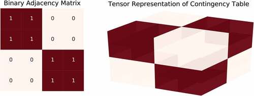
The binary variables can also be encoded as two independent Poisson variables whose sum equals to 1. Conditioned on their sum, two Poisson random variables are distributed as a binomial distribution where the probability of selecting a category is proportional to the normalized Poisson rate. The argument in equality (4) can be adapted to the adjacency matrix by considering a count tensor $X\in {\mathbb{N}}^{I\times J\times S}$

$\prod _{ij}(\mathbb{I}{Y}_{ij}=\sum _s{X}_{ijs}\}\cdot \prod _s\mathcal{P}\mathcal{O}(X_{ijs};{\lambda }_{ijs}))=\prod _{ij}\mathcal{P}\mathcal{O}(Y_{ij};{\lambda }_{ij+})\cdot \mathcal{M}(X_{ij:};Y_{ij},p_{{\lambda }_{ij:}})\}$

where $p_{{\lambda }_{ij:}}=(\frac{{\lambda }_{ij0}}{{\lambda }_{ij0}+{\lambda }_{ij1}},\frac{{\lambda }_{ij1}}{{\lambda }_{ij0}+{\lambda }_{ij1}})$ and we extend the adjacency matrix $Y$ by an additional index $s$. The index $s$ represents the possible categories of the observed data. For example, the fibers $(s=1)$ and $(s=0)$ denote the positive (1s) and negative (0s) samples of the adjacency matrix, respectively. This representation is illustrated in Figure 2 and the preprocessing steps are summarized below.

Figure 2. Count tensor representation of a binary adjacency matrix.

(1) A binary adjacency matrix $Y\in \{0,1{\}}^{I\times J}$ is observed.

(2) A dimension is added, and its corresponding count tensor $X\in {\mathbb{N}}^{I\times J\times S}$ is created where $|s|=2$ for the binary case.

(3) The observations are placed in $X$ with respect to the rule: $X_{ijs}=\mathbb{I}\{Y_{ij}=s\}$.

Initialization and Hyperparameters of BAM-MMSB

For each parameter configuration in the experiments, the variational inference step is performed several times (from 35 to 100 initializations). The one which provides maximum ELBO is chosen. However, empirically, we show that the algorithm requires a large number of runs to converge to a local maximum if started with random initializations. For this reason, we use k-means or spectral clustering for initialization purposes.

The hyperparameters of BAM are initialized according to (Cemgil et al. 2019). The allocation tensor $S$ is expected to be sparsely allocated. Thus, the hyperparameter is chosen as $\alpha (i_{1:N})\in \{0.05,0.25\}$ to induce sparsity in the allocation tensor $S$. If prior information is not provided, it is reasonable to choose uniform values for $\alpha (i_{1:N})=\alpha =\frac{a}{{\prod }_n{I}_n}$. Furthermore, the parameter $\lambda$ controls the prior expectation of the total number of tokens. Since the Gamma expectation is $\mathbb{E}[\lambda ]=\frac{a_{\lambda }}{b_{\lambda }}$, the scale hyperparameter can be chosen as $b_{\lambda }=a_{\lambda }/S_{+}$. Correspondingly, the shape parameter can be chosen as $a_{\lambda }=(({\prod }_n{I}_n)\cdot \alpha )$ so that the allocation tensor $S$ is encouraged to be sparse through the parameter $\alpha$.

Model Selection Performance

For a given latent variable model, the model selection problem corresponds to choosing the optimal number of blocks $K_{opt}$ that explains the latent structure in the observed data best. Bayesian statistics provides a principled likelihood-based approach for this task. The aim is to choose the model, which produces the largest marginal likelihood of the observed data $X$. However, the marginal of $X$ is often intractable. Therefore, we choose to approximate the marginal by its mean-field variational approximation similar to the work of Latouche et al. (Latouche, Birmele, and Ambroise 2012).

First, we perform experiments on synthetic networks. Next, the model selection performance is evaluated for real-world benchmark networks.

Synthetic Networks

To assess model selection performance in synthetic networks, we use the assortative network topology. Assortative networks have simple connectivity patterns where nodes from the same blocks connect with a probability $\in$, nodes from different blocks connect with a probability $\rho$ and $\in >\rho$. The block matrix structure is as follows:

$B=\left(\begin{array}{cccc}\in & \rho & \dots & \rho \\ \rho & \in & \hspace{0.17em}& \rho \\ ⋮& \hspace{0.17em}& \ddots & ⋮\\ \rho & \rho & \dots & \in \end{array}\right)$

The blocks of synthetic networks have balanced number of nodes among each other. Let us denote the set of blocks as $\{k_1,\dots ,k_K\}$. Balanced blocks have equal number of nodes with $|k_t|\approx |V|/K,\mathrm{\forall }t\in [K]$, where $|V|$ is the number of nodes in the network. This effect is achieved in the MMSB generative model by drawing the membership vectors ${\pi }_i\in {\mathbb{R}}^K$ for each node $i$ from uniform and sparse Dirichlet distributions as ${\pi }_i\sim \mathcal{D}(0.01\cdot {\mathbf{1}}_{\mathbf{K}})$.

In the experiments, $\rho$ is set to 0.01 and three different values are used for $\in =\left\{0.9,0.7,0.5\right\}$. Each sampled network has $|V|=40$ nodes. The number of blocks is varied as $K_{true}\in \{2,3,4\}$, but in the inference process $K$ is assumed to be unknown. For each $\left\{K_{true},\in ,K\right\}$ configuration, we sample 50 different assortative networks and estimate the optimal number of clusters $K_{est}$. The results are displayed in Table 1.

Table 1. $K_{est}$ estimations in 50 experiments for three different connectivity levels. From top to down, the connectivity parameter $\in$ takes values of $\{0.9,0.7,0.5\}$ respectively.

BAM-MMSB						MMSB
K	1	2	3	4	5	1	2	3	4	5
2	0	50	0	0	0	0	50	0	0	0
3	0	0	50	0	0	0	2	43	5	0
4	0	0	0	50	0	0	2	22	25	0
2	0	50	0	0	0	0	49	1	0	0
3	0	0	50	0	0	0	7	39	4	0
4	0	0	0	50	0	0	3	28	19	0
2	0	50	0	0	0	0	50	0	0	0
3	0	0	50	0	0	0	33	16	1	0
4	0	0	0	50	0	0	38	12	0	0

One observation for large values of $K$ is that the model tends to find one exact block and combines the rest into a big cluster. This pattern suggests that if we continue to observe Bernoulli trials for each index, or if we have more observed data, we may capture all of the true clusters. If that is not the case, then, we may apply heuristics such as scaling Bernoulli trials for each index.

We also compare the performance of BAM-MMSB with two modularity-based methods: leading eigenvector method (LEM; Newman 2006a), hierarchical modularity measure (HMM; Blondel et al. 2008) and mixture of finite mixture SBM (MFM-SBM Geng, Bhattacharya, and Pati 2019). We evaluate the performance on balanced networks with – V – = 40 nodes, number of blocks $K_{true}=\{2,3\}$. The ratio of correct estimations with respect to total estimations is reported in Table 2. We show that all the methods can estimate the number of clusters.

Table 2. Ratio of correct estimations with respect to total estimations out of 50 replicates for $\in =0.5$.

LEM	HMM	MFM-SBM	MMSB	BAM-MMSB
0.98	1	0.98	1	1

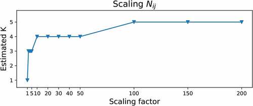
The BAM-MMSB generative model allows us to choose the number of Bernoulli trials $N_{ij}$ per each index of the adjacency matrix. Notice that $N_{ij}=1$ corresponds to the count tensor shown in Figure 2 as if there has been only one coin toss to represent an interaction. When $N_{ij}=n$ such that $n>1$, each observation model for a pair $(i,j)$ becomes a binomial experiment with $n$ trials. This procedure brings up the effect of added precision to the node classification. Therefore, we perform an experiment where the contingency tensor is scaled up with increasing $N_{ij}=n$ and $K_{true}=4$.

As $N_{ij}=n$ increases, the model’s confidence in the observations increases, and hence, the model continues to divide existing blocks and create new ones. The estimated number of blocks $K_{opt}$ for increasing pseudocounts $N_{ij}=n$ is illustrated in Figure 3. $K_{opt}$ rises quickly until it reaches to the true number of blocks $K_{true}=4$. When we continue to increase the scaling factor, it stays constant at the level of $K_{true}$ before rising gradually. For large $n$ values, the model seems to overfit and select overly complex models due to the scaled noise factor. Therefore, it seems reasonable to employ this heuristic approach for a certain data regime.

Figure 3. Estimated number of blocks $K_{opt}$ as the scaling factor $N_{ij}$ for each index is increased.

Although this method is not a statistically principled method, we see that scaling pseudocounts heuristics work well in practice for synthetic networks. Since the noise ratio is relatively large for real-world networks due to sparsity, it is not obvious how to leverage this scaling idea. As a result, we borrow a scaling heuristics idea from collaborative filtering.

Real-World Networks

In order to assess the model performance, the simulations are performed on three real-world benchmark networks: (i) Zachary’s karate club network (Zachary 1977), (ii) Lusseau et al.’s dolphin social network (Lusseau et al. 2003), and (iii) adjacency network of adjectives and nouns in the book David Copperfield by Charles Dickens (Newman 2006a).

Like most real-world networks, the networks used in the experiments exhibit sparsity having 34, 62, and 112 nodes with 156, 318, and 850 edges, respectively. As a result, our algorithm tends to select model orders with insufficient complexity. Under these circumstances, scaling Poisson counts is a heuristics solution. Figure 3 shows that scaling the contingency tensor directly may have a negative effect on the model order selection when there is inherent noise in the observations. Scaling noise drives the model to select overly complex representations, which are highly sensitive to small fluctuations. This is due to the inherent missing data in networks such that a negative sample $Y_{ij}=0$ can result from the lack of interaction or lack of information.

For the missing data problem in collaborative filtering, Pan et al. (Pan et al. 2008) proposed weighted alternating least squares (wALS) for sparse binary data sets, which contain ambiguity in the interpretation of negative samples. The idea is that each positive sample has a constant confidence level, which is higher than ambiguous negative samples. This relationship is expressed mathematically by weighting the cost of each index according to its confidence level.

We transform wALS scheme to count representations as follows. Let us denote the total negative tokens by $N_{+}^{-}$ and the total positive tokens by $N_{+}^{+}$. Following (Pan et al. 2008), we choose to use the same amount of tokens for both positive and negative samples with $N_{+}^{-}=N_{+}^{+}={\sum }_{ij}(1-Y_{ij})$. Since we have a constant confidence level for positive indices, $N_{+}^{+}$ positive tokens are distributed uniformly. Then, $N_{+}^{-}$ negative tokens are distributed according to three schemes:

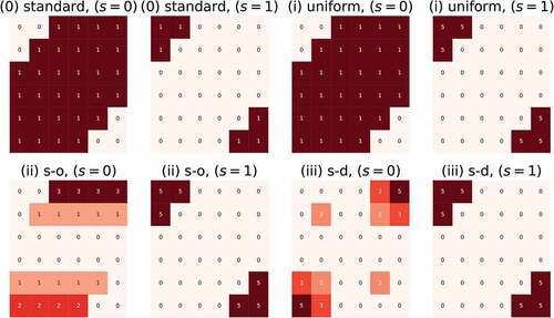
(1) Uniform: Each negative sample is represented by a single token, ($N_{ij}^{-}=1$),

(2) Source-only: Each negative sample is represented by a number of tokens proportional to the source degree, $N_{ij}^{-}\sim {\sum }_j{Y}_{ij}$

(3) Source-dest: Each negative sample is represented by a number of tokens proportional to the product of source and destination degrees, $N_{ij}^{-}\sim ({\sum }_j{Y}_{ij})({\sum }_i{Y}_{ij})$.

Notice that the tokens in $N_{+}^{+}$ are distributed evenly and stay constant in all cases. It is the negative tokens that are distributed according to distribution schemes. The negative token distributions according to cases (i), (ii) and (iii), and their difference from the count representation provided in Figure 2 are illustrated in Figure 4.

Figure 4. Weighted pseudocounts of the contingency tensor for each weighting scheme.

We performed experiments on three networks with respect to two weighting schemes: (i) uniform and (iii) proportional to source and destination popularity. The results are displayed in Figure 5.

Figure 5. The selected number of blocks for benchmark networks. The top and bottom row illustrate the results for (i) uniform and (ii) source-dest.

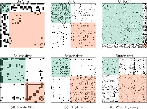
For the (i) uniform case of Karate Club and Word Adjacency networks, BAM-MMSB estimates blocks that have a leader-follower topology instead of an assortative topology. This is a well-known characteristic of the blocks inferred by standard SBMs. Specifically, the generative model tends to cluster nodes with similar degrees into the same block. It is shown that in the top row of Figure 5, this behavior results in two blocks where the green ones consisting of low-degree nodes (followers) seem to be following the red ones consisting of high-degree nodes (leaders).

Interestingly, the model behaves similarly to the degree-corrected extension of stochastic blockmodels for the (iii) source-dest case. In this case, we obtain blocks with heterogeneous degree distributions in contrast to standard SBMs. This effect shifts the estimated topologies from leader-follower to assortative in Karate Club and Word Adjacency networks, respectively. Scaling the negative pseudocounts with respect to the source and destination degrees brings up the same effect even though we do not re-weight positive samples. We opt to keep the confidence level constant for each positive observation. The estimated model orders $K_{est}=2$ are the same with (i) uniform case and commonly proposed model orders for these networks in the literature. The estimated number of clusters for dolphin data obtained with the LEM, HMM, MFM-SBM, MMSB, and the proposed method BAM-MMSB is reported in Table 3. Our results show that the proposed method, MMSB and MFM-SBM, can estimate the number of clusters, while LEM and HMM overestimate the number of clusters as 5. Moreover, variational approximations for the marginal likelihood are slightly larger for all networks with (iii) source-dest, which also suggests that degree-corrected extensions are favored over regular SBMs for these networks.

Table 3. Estimated number of clusters for dolphin data.

Method	LEM	HMM	MFM-SBM	MMSB	BAM-MMSB
Number of clusters	5	5	2	2	2

Conclusion

In this work, we propose BAM-MMSB, which replicates the generative process of the MMSB within the generic allocation framework of BAM. Our model considers the observations as Poisson tokens generated by a Poisson process and marked according to the generative process of MMSB. From a modeling perspective, two Poisson random variables can represent each Bernoulli element $Y_{ij}$ of the input matrix by adding a new index $s$ for each $(i,j)$ pair. This representation is equivalent to a Bernoulli trial when the sum is constrained to 1. This feature also provides a natural extension possibility to weighted graphs or hypergraphs for future work.

A variational Bayes algorithm is derived to solve the inference problem. The first experiment illustrates the interpretation of the model output through synthetic network examples. Next, the block recovery performance is analyzed numerically in the next experiment. As expected, BAM-MMSB displays a similar behavior to the original MMSB in the first two experiments. Furthermore, it is worth noting that uniform membership vectors and increased complexity in the block structure reduce the block recovery performance.

Our model selection algorithm approximates the marginal likelihood by a variational evidence lower bound to select the optimal number of blocks $K_{opt}$. Experimental results on real-world benchmark networks are similar to the results in the literature. However, the weighted count heuristics proposed by Pan et al. (Panet al. 2008) provide limited extendability to the task at hand since they are only heuristically motivated. A more principled approach is to integrate these heuristics into the model as random variables and infer their characteristics from the observed data (Rubin 1976).

Additionally, BAM offers a generic allocation framework, which allows for rapid prototyping of distinct generative models of discrete observations. Therefore, another natural future direction is to perform model selection not only for the model order but also across different generative models, such as tensor factorization models proposed by Schein et al. (Schein et al. 2016). In this respect, another task for future work is to compute the exact marginal likelihood via annealed importance sampling instead of approximating it.

Acknowledgments

We thank Dr. A. Taylan Cemgil (Boğaziçi University) for useful discussions. This work is supported by TÜBİTAK grant number 215E076.

Disclosure Statement

No potential conflict of interest was reported by the author(s).

Additional information

Funding

This work was supported by the Türkiye Bilimsel ve Teknolojik Araştirma Kurumu [215E076].

References

- Airoldi, E. M., D. M. Blei, S. E. Fienberg, and E. P. Xing. 2008. Mixed membership stochastic blockmodels. Journal of Machine Learning Research 9 (Sep):1981–2112.
- Bishop, C. M. 2006. Pattern recognition and machine learning. Springer, Heidelberg: Information Science and Statistics.
- Blei, D. M. 2014. Build, compute, critique, repeat: Data analysis with latent variable models. Annual Review of Statistics and Its Application 1:203–32. doi:10.1146/annurev-statistics-022513-115657.
- Blei, D. M., A. Y. Ng, and M. I. Jordan. 2003. Latent Dirichlet Allocation. Journal of Machine Learning Research (3):993–1022. http://www.jmlr.org/papers/v3/blei03a.html
- Blondel, V. D., J.-L. Guillaume, R. Lambiotte, and E. Lefebvre. 2008. Fast unfolding of communities in large networks. Journal of Statistical Mechanics: Theory and Experiment 10:10008. http://stacks.iop.org/1742-5468/2008/i=10/a=P10008.
- Brian, K., and M. E. J. Newman. 2011. Stochastic blockmodels and community structure in networks. Physical Review E 83 (1):016107. doi:10.1103/PhysRevE.83.016107.
- Buntine, W. 2002. Variational extensions to EM and multinomial PCA. In Machine Learning: ECML, eds. T. Elomaa, H. Mannila, and H. Toivonen, 23–34. vol. 2002, Berlin, Heidelberg: Springer Berlin Heidelberg. isbn: 978-3-540- 36755-0.
- Buntine, A., Wray, and Jakulin. 2006. isbn: 978-3-540-34138-3 Discrete Component Analysis. In Subspace, latent structure and feature selection,eds. C. Saunders, M. Grobelnik, S. Gunn, and J. ShaweShaweTaylor, 1–33. Berlin, Heidelberg: Springer Berlin Heidelberg.
- Canny, J. F. 2004. “GaP: A factor model for discrete data.” In SIGIR 2004: Proceedings of the 27th Annual International ACM SIGIR Conference on Research and Development in Information Retrieval, Sheffield, UK, July 25-29, 122–29.
- Cemgil, A. T., M. Burak Kurutmaz, S. Yıldırım, M. Barsbey, and U. Simsekli. 2019. Bayesian allocation model: Inference by sequential monte carlo for nonnegative tensor factorizations and topic models using polya urns. ArXiv. abs/1903.04478.
- Fosdick, B. K., T. H. McCormick, T. Brendan Murphy, T. Lok James Ng, and T. Westling. 2019. Multiresolution network models. Journal of Computational and Graphical Statistics 28 (1):185–96. doi:10.1080/10618600.2018.1505633.
- Geng, J., A. Bhattacharya, and D. Pati. 2019. Probabilistic community detection with unknown number of communities. Journal of the American Statistical Association. 114(526):893–905.10.1080/01621459.2018.1458618.
- Gerlach, M., T. P. Peixoto, and E. G. Altmann. 2018. A network approach to topic models. Science Advances 4 (7):eaaq1360. doi:10.1126/sciadv.aaq1360.
- Goldenberg, A., A. X. Zheng, S. E. Fienberg, and E. M. Airoldi . 2010. A survey of statistical network models. Foundations and Trends® in Machine Learning. 2(2):129–233. doi:10.1561/2200000005.
- Hızlı, Ç., A. Taylan Cemgil, and S. Kırbız. 2019. “Model selection for relational data factorization.” In 2019 27th Signal Processing and Communications Applications Conference (SIU), Sivas, Turkey. IEEE. 10.1109/SIU47150.2019.8977398.
- Holland, P. W., K. Blackmond Laskey, and S. Leinhardt. 1983. Stochastic blockmodels: First steps. Social Networks 5 (2):109–37. doi:10.1016/0378-8733(83)90021-7.
- Kingma, D. P., and M. Welling. 2019. An introduction to variational autoencoders. CoRR. abs/1906.02691. arXiv: 1906.02691. http://arxiv.org/abs/1906.02691
- Latouche, P., E. Birmele, and C. Ambroise . 2011. Overlapping stochastic block models with application to the French political blogosphere. The Annals of Applied Statistics. 5(1):309–36. doi:10.1214/10-AOAS382.
- Latouche, P., E. Birmele, and C. Ambroise. 2012. Variational Bayesian inference and complexity control for stochastic block models. Statistical Modelling 12 (1):93–115. doi:10.1177/1471082X1001200105.
- Le, C. M., and E. Levina. 2019. Estimating the number of communities in networks by spectral methods. arXiv: 1507.00827 [stat.ML].
- Lusseau, D., K. Schneider, O. J. Boisseau, P. Haase, E. Slooten, and S. M. Dawson. 2003. The bottlenose dolphin community of doubtful sound features a large proportion of long-lasting associations. Behavioral Ecology and Sociobiology 54 (4):396–405. doi:10.1007/s00265-003-0651-y.
- Murphy, K. P. 2012. Machine learning: A probabilistic perspective. Cambridge, MA, USA: MIT press.
- Neal, R. M. 2001. Annealed importance sampling. Statistics and Computing 11 (2):125–39. doi:10.1023/A:1008923215028.
- Newman, M. E. J. 2006a. Finding community structure in networks using the eigen- vectors of matrices. Physical Review E 74 (3):036104. doi:10.1103/PhysRevE.74.036104.
- Newman, M. E. J. 2006b. Modularity and community structure in networks. Proceedings of the National Academy of Sciences 103 (23):8577–82. doi:10.1073/pnas.0601602103.
- Newman, M. E. J., and G. Reinert. 2016. Estimating the number of communities in a network. Physical Review Letters 117 (7):078301. doi:10.1103/PhysRevLett.117.078301.
- Pan, R., Y. Zhou, B. Cao, N. N. Liu, R. Lukose, M. Scholz, and Q. Yang. 2008. One-Class Collaborative Filtering. In 2008 Eighth IEEE International Conference on Data Mining, 15-19 December 2008, Pisa, Italy, 502–11. IEEE. doi: 10.1109/ICDM.2008.16.
- Peixoto, T. P. 2015. Model selection and hypothesis testing for large-scale network models with overlapping groups. Physical Review 5 (1):011033.
- Peixoto, T. P. 2017. Bayesian stochastic blockmodeling. arXiv. preprint arXiv:1705.10225.
- Riolo, M. A., G. T. Cantwell, G. Reinert, and M. E. J. Newman. 2017. Efficient method for estimating the number of communities in a network. Physical Review 96 (3):032310. doi:10.1103/PhysRevE.96.032310.
- Rubin, D. B. 1976. Inference and missing data. Biometrika 63 (3):581–92. doi:10.1093/biomet/63.3.581.
- Schein, A., M. Zhou, D. M. Blei, and H. M. Wallach. 2016. “Bayesian poisson tucker decomposition for learning the structure of international relations.” In Proceedings of the 33nd International Conference on Machine Learning, ICML 2016, New Y ork City, NY, USA, June 19-24, 2810–19.
- Zachary, W. W. 1977. An information flow model for conflict and fission in small groups. Journal of Anthropological Research 33 (4):452–73. doi:10.1086/jar.33.4.3629752.