
 ?Mathematical formulae have been encoded as MathML and are displayed in this HTML version using MathJax in order to improve their display. Uncheck the box to turn MathJax off. This feature requires Javascript. Click on a formula to zoom.
ABSTRACT
Supervised feature selection aims to find the signals that best predict a target variable. Typical approaches use measures of correlation or similarity, as seen in filter methods, or predictive power in learned models, as seen in wrapper methods. In both approaches, the selected features often have high entropies and are not suitable for compression. This is a particular drawback in the automotive domain where fast communication and archival of vehicle telemetry data is increasingly important, especially with technologies such as V2V and V2X (vehicle-to-vehicle and vehicle-to-everything communication). This paper aims to select features with good predictive performances and good compression by introducing a compressibility factor into several existing feature selection approaches. Where appropriate, performance guarantees are provided for greedy searches based on monotonicity and submodularity. Using the language of entropy, the relationship between relevance, redundancy, and compressibility is discussed from the perspective of signal selection. The approaches are then demonstrated in selecting features from a vehicle Controller Area Network for use in SVMs in a regression task, namely predicting fuel consumption, and a classification task, namely identifying Points of Interest. We show that while predictive performance is slightly lower when compression is considered, the compressibility of the selected features is significantly improved.
Introduction
Cities are becoming increasingly smart, with more sensors producing larger amounts of data. Sensors are deployed in all aspects of city infrastructure, and in particular, they are necessary for intelligent transportation systems. Collecting data from these sensors, storing and analyzing it, presents a huge challenge for researchers. Vehicles increasingly communicate with other vehicles (V2V) and traffic management systems (V2X) to enhance both efficiency and safety (Harding et al. Citation2014; Weiß Citation2011). For example, it is possible for one vehicle to broadcast that its brakes have been applied to warn others that they are slowing, reducing the burden on a human driver seeing the brake light. Modern roadside infrastructure is also laden with sensors that measure traffic flow, pollution, and weather among other things and use transmitters to provide useful information for vehicles and their drivers (Guerrero-Ibáñez, Zeadally, and Contreras-Castillo Citation2018). For example, traffic flow beginning to slow in one section of a highway may be eased by lowering the speed limit temporarily in another, reducing the level of traffic at the bottleneck. These examples all require large amounts of telemetry data to be communicated over networks. Existing communications infrastructure cannot satisfy the required bandwidth, necessitating new communication protocols and novel approaches to data analysis.
Supervised machine learning aims to build models that map inputs to output predictions for a target variable (Witten et al. Citation2016). For example, an automotive manufacturer may wish to learn a model that estimates whether or not a vehicle is likely to have a fault in the near future. Such a model may take input data from on-board vehicular sensors but also require data from many vehicles to learn a model with sufficient accuracy. Similarly, a highways agency may wish to locate pot-holes or predict traffic jams using road sensors and vehicle telemetry data. The number of possible input features in such domains is large, and computationally, it is typically impractical to consider them all. Moreover, many features may be irrelevant to the target variable or redundant with respect to other features. Both irrelevance and redundancy can increase model complexity or cause incorrect mappings to be learned, which in turn leads to lower predictive performance. To overcome this, supervised feature selection can be used to find a subset of the features that are most related to the target variable (i.e., high relevance) but least related to each other (i.e., low redundancy) (Ding and Peng Citation2005; Peng, Long, and Ding Citation2005) or have the best performance when combined in a model (Aboudi and Benhlima Citation2016; Guyon and Elisseeff Citation2003). However, feature selection approaches generally have a bias for features that carry more information about a target variable, as these typically are the most relevant. This high information content often coincides with high entropies and poor compression, meaning that these signals are likely to be expensive to communicate and difficult to store in data centers.
This paper considers compression as a cost in the feature selection process using ideas from cost-based feature selection (Bolón-Canedo et al. Citation2014) and aims to choose features with good predictive performance as well as high compression. In particular, the paper:
introduces a compressibility factor into a variety of filter and wrapper approaches to feature selection,
performs an entropy analysis of introducing the compressibility factor into feature selection schemes based on mutual information (MI), and
assesses the selection of compressible features from vehicle telemetry data in a regression and a classification task.
Specifically, a compressibility factor is introduced into the maximum relevance (MR), minimal redundancy maximal relevance (MRMR) (Peng, Long, and Ding Citation2005), and goodness of fit (GOF) (Das and Kempe Citation2011) filter approaches, and the wrapper (Kohavi and John Citation1997) approach using linear regression (), logistic regression (
), and support vector machines (SVM). Relevant performance guarantees for greedy searches, based on monotonicity, submodularity, or weak submodularity, are provided for each of the filter methods (Nemhauser, Wolsey, and Fisher Citation1978). Although such theoretical guarantees do not extend to wrapper approaches, related assurances can be derived from those of model performance measures (May, Dandy, and Maier Citation2011). As such, wrapper methods typically achieve good performances when a suitable evaluation is used (Kohavi and John Citation1997). The proposed methods are then demonstrated in selecting features to predict instantaneous fuel consumption (FC) and to detect points of interest (PoIs) (Van Hinsbergh et al. Citation2018) using the telemetry signals available via a vehicle controller area network (CAN).
The remainder of this paper is structured as follows. Section 2 discusses related work in feature selection and compression. Section 3 details the performance measures and selection algorithms, along with any relevant performance guarantees. This is followed by an entropy analysis of MR, MRMR, and compressibility in Section 4. The selection methods are then demonstrated on collected vehicle telemetry data in Section 5. Finally, Section 6 concludes this paper and outlines future work.
Related Work
Feature selection aims to find a subset of all possible features to reduce their number while still sufficiently describing the data with respect to a particular task (Chandrashekar and Sahin Citation2014). Unsupervised feature selection generally aims to find the features that best differentiate the samples (Jennifer and Brodley Citation2004; Mitra, Murthy, and Sankar Citation2002). Typically, this relies on transforming the feature space, assessing clustering properties, or other discriminatory properties measured using heuristics (Alelyani, Tang, and Liu Citation2013).
In supervised learning, which is the focus of this paper, the three main approaches to feature selection are embedded, wrapper, and filter methods (Guyon and Elisseeff Citation2003; Jain and Singh Citation2018). Embedded methods perform feature selection as part of the learning algorithm (Lal et al. Citation2006). For example, in decision tree induction, the choice of variable on which to split nodes can be seen as feature selection. The nodes used, and their associated features, are then the selected features. Trees in random forests may also be removed if their estimated performance is poor, which may mean poor-performing features are never used in the learned model.
Wrapper methods assess feature subsets via the performances of models that use them as inputs (Kohavi and John Citation1997). This is done by comparing the performances of models learned using the same process and training samples but with different sets of input features. Wrapper methods are typically computationally expensive, as they require a machine learning algorithm to build a model for each feature subset evaluation. Filter methods, on the other hand, generally assess the performances of feature subsets using heuristics that are typically less computationally expensive. Some commonly used heuristics include similarity measures such as Pearson’s Correlation Coefficient (PCC) or MI, which can be used to estimate both relevance and redundancy of a feature set (Jain and Singh Citation2018; Witten et al. Citation2016).
In general, selecting up to features from a set of features,
, can be represented as an optimization problem (Kumar and Minz Citation2014),
where estimates the performance of a subset of these features,
, with respect to predicting the target variable,
. Ideally, all possible subsets would be evaluated to find the feature set that provides the highest performance, but the number of possible feature subsets is
, and this exhaustive search is infeasible. In practice, therefore, a more efficient combinatorial search algorithm is applied.
Possibly, the most common search strategy is the forward greedy search (Kumar and Minz Citation2014), which selects the feature, , that satisfies a condition,
,
in each of iterations. The search begins with no selected features,
, and so initially the feature with the highest individual performance is selected. It is typical that during this first iteration,
. In the subsequent
iterations,
is the performance of the already selected features, and the feature that increases the performance most is selected. The search stops when a stopping criterion is met, such as when a given number of features are selected or if the performance score decreases after selecting a new feature.
If the performance measure is both monotone (i.e., increases with ),
for all , and submodular (i.e., has diminishing returns),
for all , then the solution of the forward greedy search is within
(
) of the optimal. The consequences of submodularity are also used in the lazy greedy search algorithm (as described in Section 3.6), which maintains a sorted list of upper bounds on the marginal gains to reduce the number of evaluations of
(Minoux Citation1978). If the performance measure is submodular but non-monotone, alternative greedy algorithms with different performance guarantees can be used (Buchbinder et al. Citation2015; Feige, Mirrokni, and Vondrak Citation2011), and the submodularity ratio (Das and Kempe Citation2018) can be used for set functions that are monotone but not submodular.
Two advances to the greedy algorithm include the distributed greedy and stochastic greedy searches (Khanna et al. Citation2017; Mirzasoleiman et al. Citation2015). In each of these, multiple searches are applied to different subsets of the full feature set. In distributed greedy search, the subsets are generated by sampling the features without replacement, whereas in stochastic greedy search, the sampling is performed with replacement. The results of the multiple searches are combined into an interim result set, on which another greedy search is applied to find the final result. Alternatively, the feature subsets can be combined by taking their intersection (Nagpal and Singh Citation2018).
Other optimization approaches include particle swarm optimization (PSO), which iteratively updates candidate vectors in a population based on both local and global information (Kennedy and Eberhart Citation1995). For feature selection using binary PSO, a candidate vector is a probabilistic representation of a feature being selected, that are collapsed onto either or
for feature set evaluation using a random threshold (Chuang et al. Citation2008). Similar to this, brain storm optimization iteratively clusters candidates, generates new ones, and selects those with the best performance for the next iteration (Papa et al. Citation2018). Differential evolution approaches also iteratively create new populations through a process of mutation, crossover, and selection (Zhang et al. Citation2020).
Feature selection is often characterized as a compression method, as it reduces the data that must be processed by machine learning algorithms and models. This has several advantages, including reducing model complexity and improving performance, but selected features often have high variances and entropies that typically coincide with good predictive performance (Guyon and Elisseeff Citation2003). This bias toward high entropy features limits the data compression that can be achieved with those that are selected. It may be the case, particularly with the high redundancies found with vehicle telemetry and city data, that some features with lower entropies and better compression may provide comparable predictive performances (Taylor, Griffiths, and Mouzakitis Citation2018).
To achieve both these competing aims, namely selecting high quality features that have good compression, this paper adopts ideas from cost-based feature selection. A simple approach is to introduce a cost factor, , into the optimization problem (EquationEquation 1
(1)
(1) ) as follows (Bolón-Canedo et al. Citation2014):
where is a cost weighting parameter. A similar approach is to sum the costs of individual features to estimate the cost of the feature set (Jiang, Kong, and Li Citation2021). Costs of features can arise from observing or measuring them (e.g., in using expensive medical machinery), or computational costs (e.g., in extracting features from large images).
Other approaches include searching for a pareto-optimal solution where no criteria can improve without worsening another (e.g., (Hancer, Xue, and Zhang Citation2018; Zhang et al. Citation2019, Citation2020)). Typically, such mutliobjective optimization approaches focus on the competing aims of minimizing the number of selected features vs predictive performance, but Hancer et al. (Hancer, Xue, and Zhang Citation2018) demonstrated it for multiple feature performance measures (including MI relevance and redundancy). While such approaches may be applicable to the objectives of predictive performance and compression, they do not enable an investigation of the trade-off between them. As such, this paper employs a cost-weighting parameter that enables full control over the relative importance of compression, measured using a compressibility factor outlined in Section 3.1.
Data compression aims to remove redundancy, thus making the data representation smaller, in such a way that it can be restored (Salomon and Motta Citation2010). Characteristics of city and vehicle telemetry data, including temporal consistency, noise, and signal redundancy, all support good compression. While signal redundancy is removed in performing feature selection, noise and temporal consistency are not removed and must be considered using other kinds of data compression. There are two broad categories of data compression, namely lossless and lossy.
Lossless compression aims to compress the data in such a way that the uncompressed version is indistinguishable from the original (Salomon and Motta Citation2010). Typically, lossless compression inspects the frequencies of symbols and looks for repeating symbols or sequences of symbols in the data stream. Perhaps the most simple method of compression is run-length encoding, in which symbols are encoded along with their number of consecutive repetitions. For example, the string ‘AAAABBA’ can be encoded as ‘A4B2A1.’ Two other notable lossless compression algorithms are LZ77 dictionary encoding (Ziv and Lempel Citation1978) and Huffman coding (Huffman Citation1952). LZ77 uses a sliding window and searches for repeating sequences, which are encoded as the length and location of its first occurrence in the window. Huffman coding produces a variable length prefix-code defining the path to the encoded symbol in a Huffman tree. Symbols that occur with higher frequencies are located closer to the root node in the tree and thus have shorter Huffman codes. Taken together, LZ77 and Huffman encoding make up the DEFLATE compression algorithm (Deutsch Citation1996), which is the basis of the ZIP file format.
Although lossless compression guarantees that the decompressed stream is the same as the original, lossy compression relaxes this constraint and aims only to minimize information loss. In particular, lossy compression aims to keep information where it is important and lose information where its loss will not be noticed. In MP3 audio compression, for example, the high frequencies above the human hearing range are removed. For vehicle telemetry data, similar components of the signals can be removed if they are not useful to further analysis. Some signals such as vehicle speed, for example, contain noise that may even be detrimental to analyses. Such approaches to separating informative and noise components of signals include the discrete wavelet transforms (DWT) (Addison Citation2017), the discrete Fourier transform (DFT) (Bailey and Swarztrauber Citation1994), the discrete cosine transforms (DCT) (Ahmed, Natarajan, and Rao Citation1974).
The DWT operates by extracting two signals that are each half the length of the original (Addison Citation2017). The first represents an approximation of the original signal and is referred to as the low frequency (LF) component. The second is the high frequency (HF) component and is a representation of the detail in the original signal. The LF and HF components are produced by a convolution of the original signal with wavelet kernels, followed by a down-sampling by a factor of 2. Typically, the HF component contains many small values and can be considered the noise component of the original signal. By quantizing this component and applying a threshold, many of these small values become zero and can be encoded very efficiently using lossless compression methods such as run-length encoding. This quantization introduces errors into the signal when it is reconstructed, but the error is minimized because only the HF component (detail) is affected. This process can be performed recursively to the LF component, further increasing the potential for lossless compression of the coefficients.
This paper focuses primarily on lossless compression, but the methods are also applicable to lossy compression approaches such as DWT.
Feature Selection
To consider the compression of features as a cost during their selection (Bolón-Canedo et al. Citation2014), a compressibility factor is introduced into the feature selection process alongside the performance metric, , of a feature set,
. This compressibility factor is detailed in Section 3.1, followed by its introduction to filter methods in Sections 3.2–3.4, and the wrapper method in Section 3.5. These feature selection approaches were chosen because of their simplicity and existing adoption in the literature and practice. Their range also demonstrates that compression can be considered generally in feature selection. Finally, Section 3.6 describes forward greedy and lazy forward greedy searches used to find the subset of features that maximizes the performance measure,
.
Compressibility Factor
The compressibility factor, , is defined as the mean compressibility over a set of features,
,
where is the compressibility of the individual feature,
. Compressibility of an individual feature can typically be assessed using entropy, but this is difficult to compute for vehicle telemetry signals, which are not independent and identically distributed. We therefore adopt a more direct approach and measure the space savings achieved by a compression algorithm on training samples,
where is the number of bits in the compressed data and
is the number of bits in the original. This measure is larger for variables that are more easily compressed than those that do not compress well and typically has a range of
. Therefore, this compressibility measure should be maximized to minimize the impact of poor feature compression.
Due to the pigeon-hole principle, a lossless compression algorithm may increase the number of bits in the data in some circumstances, leading to having a value greater than
. To mitigate this, a compression algorithm can output the original data if its size would be increased and prepends a single bit to signify whether or not this is the case. If the bit has a value of
, all subsequent data is equal to the original (i.e., it was not compressed), and otherwise the subsequent data was compressed by the algorithm and should be decompressed. Therefore, in general,
has a range of
, where
.
In the simulations performed for this paper, the compressibility is measured using DEFLATE for all features, which in the worst case increases the required storage by at most three bits per block. Different features are more suited to different compression methods, however, so it may be beneficial to employ a compression strategy targeted toward the particular features being considered. For example, DEFLATE may be applied to some features and DWT to others, or groups of features may be considered together in a more comprehensive compression strategy. These approaches incur higher computational costs during feature selection, however, compared to applying the same compression method to each feature individually. We therefore leave the development of a more sophisticated estimate for the impact of poor compression to future work.
Maximum Relevance (MR)
To assess the relevance of a feature set, the individual feature relevancies can be aggregated,
where is the MI between feature,
, and the target,
. Unfortunately, the mean is not monotone and is not submodular in general. To overcome this,
is redefined as a summation, which is both monotone and modular,
In a forward greedy search, this is equivalent to selecting the feature, , that satisfies,
in each iteration.
Theorem 1 is monotone and modular.
Proof 1 ,and any summation of a set of positive numbers is monotone and modular.
Theorem 2 The final set, ,found using a stable forward greedy search is the same when using either the mean of individual signal performances,
), or their summation,
).
Proof 2 In the iteration,
,and
. Given
,let
be the feature selected using
,and let
be that selected using
. Using
,
Using ,
and so both and
Finally, because the search is stable (i.e., tie breaks are decided deterministically),
. Therefore, in each iteration of a forward greedy search, the same maximizing feature,
, is selected using either
or
.
Corollary 1 Using a stable forward greedy search to maximize the summation or mean
yields the same optimal result for MR.
To maximize the compression of selected features, the compressibility factor must also be maximized. The combination of and the compressibility factor (
) can be defined as,
where a weighting parameter, , allows the level to which compression is considered during the selection process to be varied. The smaller the value of
, the less compression is considered. In particular, a value of
means that
is equivalent to
selection. As with
,
can be written as a monotone and modular summation,
which results in the same optimal final set as when using stable forward greedy search (see Proof 2). Such a forward greedy search selects the feature,
, that maximizes,
in each iteration.
Minimum Redundancy Maximum Relevance
The redundancy of a feature set can be assessed as the mean of all pairwise feature similarities, measured using MI,
which, in , is to be minimized in the performance function, for example,
As with ,
can be written as a summation,
which is equivalent to selecting the feature, , which satisfies,
in each iteration of a stable forward greedy search.
In this form, is neither submodular nor monotonic. Having said this, the
criterion (EquationEquation 18
(18)
(18) ) is equivalent to the max-dependency criterion when one feature is selected at a time (Peng, Long, and Ding Citation2005), as in forward greedy search. While
aims to minimize redundancy between features and maximize their relevance to a target variable, it does not consider the joint probability distribution of the variables. Max-dependency aims to directly maximize the joint dependency between the features and the target variable (Peng, Long, and Ding Citation2005). Direct analysis of the joint probability distributions is computationally expensive, however, so
is a useful alternative when using forward greedy search. Furthermore, max-dependency is easily shown to be monotone (i.e., adding an input variable does not decrease the MI dependency with the target). Therefore,
results in the same selected features as with max-dependency, which provides an approximation guarantee of
.
Finally, the compression factor can again be introduced as,
which is equivalent to selecting the feature, , that satisfies,
in each iteration of a stable forward greedy search.
Goodness of Fit
If two features are poor individual predictors (i.e., they each have low relevance to the target) but can be combined in a model to have good performance, they should be selected. and
are both unable to capture these kinds of feature interactions (although adaptations using conditional MI exist (Herman et al. Citation2013)). Alternatively, such feature interactions are captured by assessing the GOF,
, of features in a model,
produced by fitting the features to target
using the learning algorithm
. Goodness-of-fit measures how closely the model maps the input data,
, to the target variable,
. In regression tasks, a linear regression model is often used alongside the
goodness-of-fit measure. In general, any model and GOF measure can be used. For example, in a classification task, a Naïve Bayes or SVM classifier can be used alongside the accuracy or area under the receiver operator characteristic curve (AUC) as a measure of fit (Witten et al. Citation2016). The performance of a feature set using GOF then has the form,
If the measure for GOF is a non-negative monotone set function, an approximation guarantee is provided via the submodularity ratio,
which is the minimum ratio of increase in performance when adding individual elements of one subset, , to another,
, compared to adding all elements of
to
at once (Das and Kempe Citation2011, Citation2018). Specifically, with linear regression and
, forward greedy stepwise selection provides a lower bound approximation of
. A special case of this approximation is when the GOF is measured using a sub-modular function, in which case
and the lower bound approximation is
.
For the regression task investigated, a linear regression model is used, , of the form,
where is the linear coefficient and
is the error term. GOF is measured using
,
where is the expectation, or mean, of the variable. In this GOF selection for regression (
), therefore, the performance measure is
For the classification task, binomial logistic models (Cox Citation1958) are used,
which output the likelihood of the target variable having a value of . Using this likelihood, the AUC,
, is calculated as a measure for goodness of fit. Thus, goodness of fit for classification (
) uses the performance measure
While this suffices for the binary classification task used in the evaluation for this paper, performing stepwise selection with multi-class target variables requires a multi-class learning algorithm, such as a decision tree or naïve Bayes. Another possible approach is to transform the target into multiple binary variables and learn multiple binary classification models to be combined in an ensemble (Fürnkranz Citation2002).
To consider compression in both the regression and classification tasks, the compressibility factor is again added to the performance metrics. The and compressibility (
) performance metric is then
and for and compressibility (
), it is
Wrapper (W)
The wrapper approach to feature selection is similar to GOF, but goodness of fit is replaced by model performance, measured from data not used when fitting the models (Aboudi and Benhlima Citation2016; Guyon and Elisseeff Citation2003). As feature selection is performed using the training data, the training data is further split into a selection-training portion, , to learn models using different feature sets, and a selection-testing portion,
, to assess their performance. It is typical for this selection-testing portion to be referred to as hold-out or validation data. A selection-training portion that is too small may lead to poorly fit models that are not indicative of the performance of the feature set, while one that is too large will leave too few samples in the selection-testing portion for a reliable performance estimate. Alternatively, the training data can be split into several folds, for a
-folds cross evaluation of each feature set, but of course this increases the computational requirements of the already computationally expensive wrapper approach. In this paper, the first half of the training samples temporally make up the selection-training portion, and the remainder make up the selection-testing portion.
Any learning algorithm, , can be used in a wrapper, although usually it is the same model that is to be used on the final set of features. For example, if features are being selected for use in SVM, then a SVM is the most appropriate method for use within the wrapper during the selection process. A large number of models are typically learned during wrapper selection, and some learning algorithms require a large amount of computation to learn each model. Therefore, the computational requirements of a learning algorithm may also be a consideration when adopting the wrapper selection approach, in particular with large numbers of features from which to select. In some cases, a two-stage feature selection process may be performed that uses a filter to reduce the number of features significantly before applying a wrapper to reduce the feature set further (Peng, Long, and Ding Citation2005).
To assess the performance of a set of features, , a model,
, must first be learned using the selection-training portion,
,
This model is then applied to the selection-testing portion, , to produce a set of outputs,
which are then compared to the observed values, , to estimate the performance using a performance measure,
Alternatively, this can be written by defining the model outputs using a partial function of the learning algorithm,
Again, compression can be considered by adding the compressibility factor to the performance measure,
The submodularity of the wrapper approach cannot be guaranteed, in general, because the model is learned and evaluated using different sets of data. If the training data is independent and identically distributed (IID) and sampled in a stratified manner, a performance guarantee similar to that provided by the submodularity ratio can be achieved when using linear regression. Time series data, however, is not IID, and so no such guarantees can be provided for the data used in this paper.
In our evaluation for the regression task, is used as a model performance measure and both linear regression (i.e.,
), referred to as
, and SVM regression (i.e.,
), referred to as
. For the classification task, AUC is used along with logistic regression (i.e.,
), referred to as
, and SVM classification (i.e.,
), referred to as
. In all cases, compression is included by adding the compression factor; therefore, for linear regression and
with compression (
), the performance measure is
and for SVM regression with compression (), it is defined as
The performance measure for logistic regression with compression () is defined as
and finally, for SVM classification with compression (), it is defined as
Search
In feature selection, the aim is to find the subset of features that maximizes the performance metric, . Naively, this is done by evaluating the performance metric for all possible subsets of features, but in reality, there are too many subsets for this to be feasible. For instance, there are
different subsets of size
when selecting from
features. The forward greedy search is outlined in Algorithm 1 and iteratively selects the feature that maximizes the marginal gain in performance until
features have been selected. In each iteration,
is computed for each unselected feature, meaning that
feature set evaluations are performed when selecting
features from a set of
features. While this is usually computationally feasible for filter approaches, the feature set evaluation in the wrapper approach is significantly more expensive, and so a more efficient search is required.
Algorithm 2 outlines the lazy forward greedy search algorithm (Minoux Citation1978). To avoid computing for every unselected feature in each iteration, lazy forward greedy search prioritizes the features with good performance in previous iterations. Specifically, the feature,
, with maximum observed marginal gain,
, is tentatively selected and evaluated to recompute and update its marginal gain,
It is possible that this new marginal gain is no longer the maximum observed. In this case, the next feature, which now maximizes the marginal gain, is tentatively selected and evaluated. This process is repeated until a feature is tentatively selected for a second time, where it is selected and added to . During the first iteration, when
, the algorithm requires that
. In subsequent iterations,
is the performance of the already selected features.
Table
Table
Entropy Analysis
MI is typically defined as
but is equivalently defined using entropies,
where and
are the marginal entropies of
and
,
is their joint entropy, and
and
are conditional entropies. The marginal entropy,
, also provides a lower bound on the number of bits required to represent some data,
, i.e., the best compression achievable. Although compression algorithms such as DEFLATE often require a larger number of bits than this bound in practice,
is still a useful theoretical tool for assessing compressibility. In particular,
is lower when
can be represented by fewer bits when compressed than when
is difficult to compress and, thus, has similar properties to the compression ratio. In this section, we use entropies to analyze the relationships between relevance, redundancy, and compression in
,
,
, and
.
selects the feature that satisfies the condition,
, in each iteration, which is defined using entropy as
Similarly, is defined as
as
and as
Each of these equations is a linear sum with four terms, of which some are maximized (i.e., they are positive) and some are minimized (i.e., they are negative). shows the coefficients of these terms in each of the four information-based feature selection methods. While is always maximized with a factor of
, it can be ignored as it is a constant throughout the selection process because the target,
, is fixed.
Table 1. The quantities of entropy that are maximized in each of the entropy based criterions.
In all the equations relevance is maximized, which in each equation is represented by (i.e., the conditional entropy of
given
is minimized). Intuitively, this is minimizing the unknown quantity of
given the information in
, represented as the intersections of
and
with
Venn diagram in ). In this example,
has a larger intersection with
than
(i.e., more of
is known given
than
).
Figure 1. Entropy Venn diagrams.
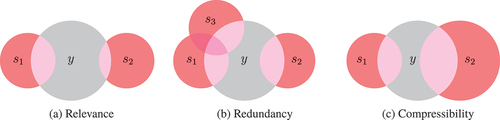
In and
, redundancy is minimized using the term
(i.e., the mean conditional entropy of
given the already selected features is maximized). This term aims to minimize the information overlap, or redundancy, of the selected features. ) shows three variables,
,
and
, each with the same size of intersection (relevance) with the target variable,
. After selecting
,
is preferred over
as its intersection (redundancy) with the already selected features,
, is smaller.
Finally, in and
, compressibility is maximized by
(i.e., a portion of the marginal entropy of
is minimized). This is effectively minimizing the amount of information a feature carries. The Venn diagram in ) shows two variables,
,
with equal overlaps with the target variable (relevance), and no redundancy. The smaller set,
, representing lower entropy, is more compressible than the larger set,
, representing a higher entropy, and so in this case, therefore,
is preferred over
.
The effect of is demonstrated using simulated data in , for which 100 samples were generated, with the first 50 samples having a target value of
and the target value of the remaining 50 samples being
. Nine features were then generated with fifty zero values and fifty non-zero values, to have different relevancies, redundancies, and entropies. In the first set of three features, the non-zero values were at samples 5 to 55, in the second set of three features the non-zero values were at samples 10 to 60, and in the final set of three features they were at samples 15 to 65. This ensures that the features have different relevancies to the target and different redundancies to one another. In each set, the non-zero values of the first feature were either 1 or2, in the second feature they were either 1, 2, or 3, and in the third feature they were either 1, 2, 3 or 4 each chosen uniformly at random. The more values a feature takes, the more entropy it has in general.
Figure 2. Demonstration of (a) vs
and (b)
vs
.
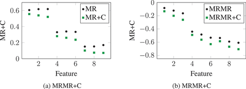
) shows the mean ,
(with
) over ten generated datasets. The features with the most non-zero values when
(features 1, 2, and 3) had the highest relevancies (measured using
), whereas those with fewest non-zero values when
(features 7, 8, and 9) had the lowest relevancies. Features with the same set of non-zero samples but that took more values also had higher
(e.g., feature 3 had a higher relevancy than feature 1), even though they contain the same information about the target variable,
. With
, those features that had more values but the same set of non-zero values were considered of lower importance, since the entropy of features is also considered.
) shows the same results for , and
(with
). Redundancy for each feature was computed as its total MI to the other eight features. Here,
also prefers features with fewer values, as they have less chance for having values in common. This is, however, not true in general, and
still had an effect in reducing the
scores of the features that took more values. In fact, a feature with more non-zero samples when
and higher relevance (feature 6) had a slightly lower score than a feature with fewer non-zero samples (feature 7) once compression was considered. This means that a feature with lower predictive performance may be selected over a feature that may provide better predictions, but to the benefit of compression.
Results
In this section, the results for the feature selection approaches described in Section 3 are provided. The results were obtained using the Location Extraction Dataset (LED) (Van Hinsbergh et al. Citation2018). The LED consists of over 1900 vehicle telemetry signals collected over 72 journeys in an urban environment, while performing various pick-up and drop-off scenarios. Data was sampled at 10 Hz and the mean length of each journey was 19.7 minutes, the standard deviation of journey lengths was 8.2 minutes, and the range was 29.1 minutes. All signals with names containing the strings ‘time’ and ‘minutes’ were removed prior to any feature selection or model learning, as they were found to be detrimental to the results due to each sample having a unique value.
One regression task, namely estimating the instantaneous Fuel Consumption (FC), and one classification task, namely detecting Points of Interest (PoI), were constructed using the LED. For FC, all signals containing the string ‘fuel’ or ‘torq’ were removed from the data, because these signals can be used to achieve high performances in simple models using one feature. In both tasks, training data was made up of the samples from ten journeys sampled randomly without replacement, and testing data was made of different ten journeys, again sampled randomly without replacement. The data was split temporally into equally sized blocks of samples, from which the mean (if continuous) or modal (if categorical) value was extracted. The block size for the FC task was 10 samples (1 second), and for the PoI task a block size of 50 samples (5 seconds) was used. These block sizes were chosen as they provided the most interesting trade-off for predictive performance and feature compression, and provided training and testing datasets with a mean number of samples of about 12000 for the FC task and 5200 for the PoI task.
Signals were selected from the training data using incremental search, maximizing the performance measures listed in . and
are applied to both the regression (FC) and classification (PoI) tasks, whereas
,
, and
are used for the regression task only, and
,
, and
are used for the classification task only. In both tasks, each performance measure was applied in both forward greedy and lazy forward greedy searches, and the number of feature set evaluations (applications of the performance measure) was recorded.
Table 2. Feature selection performance measures investigated in the evaluation.
For the and
methods the variables were discretised in order to estimate the integrals when computing MI (EquationEquation 43
(43)
(43) ). Specifically, the features in both tasks were discretised by learning a decision tree for each input feature using Gini’s impurity as a split criterion (Breiman Citation2017), and taking the cut points of nodes in the tree as discretization intervals. To obtain a discrete target variable in the regression task, Matlab’s histcounts functionFootnote1 was used to find suitable discretization bins. Following feature selection, the original continuous features and target variables were used in model learning and evaluation.
The selected features were used to train a SVM that predicted the target variable. Predictions were then made for each sample in the testing data, which were compared to their observed values to assess the model performances. The scores are presented for the regression task, and in the classification task AUC is used. Mean Absolute Error (MAE) and the F1 score results are available in supplimentary material. Finally, the overall compression was measured on the testing data for the selected features, using DEFLATE and DWT. The results presented are the mean performances over ten train-test cycles, and error bars show the standard errors.
Predictive Performance
shows the maximum performances for the regression task when selecting up to (a) 5, (b) 10, and (c) 15 features with different values of the compressibility factor weight,
. With up to five features,
and
had poor performances, with
, but performed significantly better when selecting up to ten or fifteen features. In fact, with up to ten or fifteen features,
had significantly the best performances when compared to the other selection methods for any value of
. The
performances of
,
, and
either did not change or increased only marginally when selecting up to ten or fifteen features compared to five features.
Figure 3. performances for the FC task.
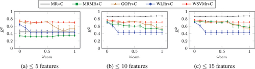
In almost all cases, giving greater consideration to compression (i.e., larger values of ) led to the selection of features with worse performances. One exception was
, where
performances remained the same with different values of
.
,
, and
, on the other hand, were affected significantly by the value of
, with
performances decreasing by up to
when comparing
and
for the same number of features.
was less affected by increasing
, with the maximum achieved
performance only decreasing slightly between
and
. Interestingly, each selection method was affected for different ranges of
. For instance,
decreased in performance with low values of
and then was unaffected by increasing
further, whereas performance was maintained by
and
until
. This may be as a result of the different ranges and distributions of the feature set performance measures, indicating that the effect of
is dependent on the performance measure being used.
The maximum performances for the classification task, PoI, are shown in when selecting up to (a) 5, (b) 10, and (c) 15 features with different values for
. As with the regression task, the performances when predicting PoIs improved with the number of features selected for
and
. For
,
, and
, the
performances however did not increase when selecting more than five features. The highest
performances were attained by
,
and
, followed by
.
Figure 4. performances for the PoI task.
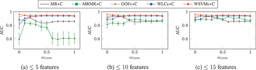
Unlike in the regression task, the consideration of compression actually improved the performance of the features selected for the PoI task in some cases. In particular, the performance increased significantly when selecting up to 5 features with
with
compared to
. Likewise,
increased with larger values of
for
, which had the worst performance of all selection methods investigated. This is indicative of overfitting due to their use of MI, which is prone to selecting high entropy features at the cost of their generalizability to new data (Taylor, Griffiths, and Bhalerao Citation2015). The consideration of compression is likely reducing this bias in MI and leading to the selection of features that are less specific to the training data.
The and
selection methods, which do not rely on MI, were less affected by the value of
, but were still improved for increased values of
. The
performance of
increased from
(with
) to
(with
), and for
it increased from
when
to
when
. For
however, the
performances decreased slightly with higher values of
.
Compression Performance
(FC task) and (PoI task) show the number of bytes required to represent the best performing features when selecting up to (a) 5, (b) 10, and (c) 15 features, using the DEFLATE compression algorithm, with a compression level of 6. For the FC task, the number of bytes is shown for the feature set that achieved the highest in each case, and for the PoI task the feature set with the highest
was used. In both tasks, more features required more bytes to represent them. In many cases, however, the maximum predictive performances were achieved by fewer than five or ten features, so the number of bytes remained the same when selecting up to ten and up to fifteen features. In particular, when
, the number of bytes required to represent features selected using
was the same when selecting either up to five, ten, or fifteen features, as were their performances.
Figure 5. DEFLATE bytes performances for the FC task.
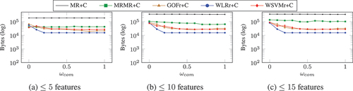
Figure 6. DEFLATE bytes performances for the PoI task.
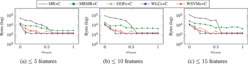
In the PoI task, the number of bytes required decreased as increased for
. Interestingly, this was predominantly when
, which is where the predictive performance also improved (). This is more evidence that
was overfitting to the training data in the PoI task, due to selecting high entropy features.
Although achieved the best performances in the FC task (), the features it selected had significantly the worst compression in either task. For example, selecting ten features using
when
required
when using DEFLATE, whereas selecting ten features using
required only
. Similarly, for the PoI task,
with
required
to represent the top ranked ten features, whereas
required only
. Features selected by
also required significantly more bytes than did the goodness of fit and wrapper approaches. Furthermore, the number of bytes required to represent features selected by
and
for the FC task were not affected significantly by the value of
, whereas the number of bytes required decreased as
increased for all other selection methods (
,
, and
). In particular,
, which had the second best performances for the FC task, required significantly fewer bytes when
than when
, with only a marginal decrease in predictive performance. The decrease in bytes was largest for
and
between
and
, and when
the number of bytes did not change significantly.
As in the FC task, the number of bytes required by features selected using and
decreased as
increased when
, and with
the number of bytes required did not change significantly. The number of bytes required by features selected using
continued to decrease with increased values of
in all cases investigated, to be similar to that required by
.
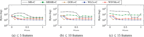
The number of bytes required to represent the selected features using the DWT are shown in for the FC task, and in for PoI. The DWT transform had two layers, each using the db5 wavelet, with a quantization level of and threshold of
. The resulting coefficients were then compressed using DEFLATE with a compression level of 6. The results in both FC and PoI reflect those found when compressing the features using DEFLATE only, but DWT achieved better compression in all cases. In both tasks more bytes were required when selecting more features. In the FC task,
was again unaffected by the value of
, and
and
had better compression with higher values of
. In the PoI task, the number of bytes required by features selected using
decreased as
increased for small values of
. In this case, however, the number of bytes required by features selected by
increased with
, and only decreased again with
.
Figure 7. DWT bytes performances for the FC task.
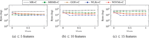
Figure 8. DWT bytes performances for the PoI task.
Lazy Evaluations
presents the maximum performances (by ) of the selection methods when applied in (a) forward greedy and (b) lazy forward greedy searches to select features for the FC task. The performances for
are not displayed in these tables, as it selects the same set of features when using either forward greedy or lazy forward greedy search. Features selected using the filter methods,
and
, tended to have worse performances when forward greedy search was employed than when using lazy forward greedy search. Although for some values of
,
performances for
with lazy forward greedy were higher than with forward greedy, the
s were still higher. For
the decrease in both
performance and increase in
from forward greedy to lazy forward greedy was significant. As a result, even though fewer bytes were required, lazy forward greedy is not appropriate when using
to select features for the FC task.
Table 3. Best performances (by ) in the FC task selecting up to 15 features using (a) forward greedy and (b) lazy forward greedy search.
Whereas the performances of when using lazy forward greedy tended to be lower than for forward greedy, the features selected required fewer bytes to achieve the maximum
score. When
, for example,
were required to achieve an
of
with forward greedy and
to achieve
with lazy forward greedy. This particular difference was predominantly due to forward greedy selecting six features whereas lazy forward greedy selected five, but to select five features with
forward greedy still required
, and also achieved a lower
performance of
. This is likely as a result of extra redundancy in features selected using lazy forward greedy, which ranks features based on their performance in previous rounds to expedite the search, rather than assessing all features in each round as in forward greedy. Because features that are promising in one round are prioritized in the next, features selected in consecutive rounds may be good in similar ways and be redundant, making their combination more easily compressible. While this is accounted for in the performance metrics, such as
and
, it is more challenging due to the reduced lazy search.
The performances of the wrapper methods, and
, were again worse in general when lazy forward greedy was used, especially with small values of
. Also in these cases, fewer bytes were typically required by the features selected. With larger values of
, however,
had better performances and required more bytes with lazy forward greedy than forward greedy. This was likely as a result of the peak performance when using forward greedy being achieved with only one feature in these cases, which is a clear sign of overfitting during feature selection. Features selected by
also required more bytes when lazy forward greedy was used than when using forward greedy, and also achieved marginally worse performances.
The maximum performances (by ) for the PoI task are presented in for (a) forward greedy search and (b) lazy forward greedy search. Again, fewer bytes were typically required to represent features selected using lazy forward greedy than were required when using forward greedy. In most cases, lower
and
performances were also achieved by lazy forward greedy. For example,
had worse performance in both
and
for any value of
, and
and
had lower
s. However,
and
did have slightly higher
performances in some cases.
, on the other hand, improved in both
and
performances while also requiring fewer bytes.
Table 4. Best performances (by ) in the PoI task selecting up to 15 features using (a) forward greedy and (b) lazy forward greedy search.
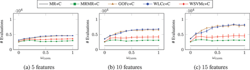
In general, lazy forward greedy selected worse features than did forward greedy, but the advantages of lazy forward greedy lie in computational efficiency while still selecting adequate features. show the number of feature set evaluations performed when using lazy forward greedy with each of the search methods when selecting (a) 5, (b) 10, and (c) 15 features. For all search methods except , the number of feature set evaluations increases with
. The most simple way to implement
is to evaluate each feature individually and produce a single ranking, from which the top features are selected. In both the FC and PoI tasks, the methods using linear regression had the most feature set evaluations, in particular for larger values of
. While
had the fewest feature set evaluations,
had a similar number and
only required around twice as many.
Figure 9. Number of feature set evaluations for the FC task.
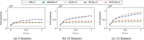
Figure 10. Number of feature set evaluations for the PoI task.
Summary
In summary, the following conclusions can be drawn from these results.
Considering compression led to the selection of features with worse predictive performances in general, but that required fewer bytes when compressed.
In the FC task,
had best performances with up to 10 or 15 features to achieve it and required the most bytes to represent them.
The next best performances in the FC task were achieved by
In the PoI task,
Using forward greedy generally provided better performances than lazy forward greedy, but in some cases the selected features required more bytes when compressed.
When considering compression of selected features, there is a trade-off against performance. In some cases, the lower predictive performance of a feature set may be acceptable when considering the significant improvement in compression. For example, in the FC task when selecting features with , it is possible to reduce the compressed size of the features from
to
while only reducing the
performance by
and increasing the
by
. In some applications, the
improvement in compression may warrant the small increase in error.
required selection of more than five features for good predictive performances, and they had the poorest compression (i.e., they required the most bytes) of all the methods. The features selected using
for the FC regression task had higher
performances than those selected by any other method, when more than five features were selected. The compression performances of the features selected by
was also unaffected by
in this task. For the PoI classification task, the features selected by
had good AUC performances when compression was considered with small values (but greater than
) of
, but poor performances with larger values.
also required the fewest feature evaluations of any method investigated when using a lazy search. In regression tasks where compression is not important, therefore,
may be most appropriate, especially when the number of feature set evaluations is to be minimized. However, this is unlikely to be the case in general as it ignores feature redundancy (Guyon and Elisseeff Citation2003).
required more features for good performance than did most other methods, only having comparable performance when
features were selected. The selected features also had poorer compression, requiring almost
more bytes than all other methods except
when compression was considered during selection. When using lazy evaluations, however,
required fewer than half the number of evaluations of other methods except
.
The linear regression wrapper had poor performance in the regression FC task for any value of . In the classification PoI task, the AUC performances achieved by features selected using
improved when compression was considered during selection. With
, AUC performance was then unaffected, and the features selected required the fewest bytes of all methods when compressed.
The two remaining approaches, based on and
had similar results in general, only differing for the FC regression task for larger values of
. For such values of
, the
performances of
decreased significantly as
increased, whereas those of
were much less affected. The features selected by either of these methods had the highest predictive performances (except
with FC) of any method investigated, and the effect for small values of
was small. Their compression performances were also similar, and both methods were outperformed only by
in the FC regression task when assessed using DEFLATE (they were similar when using DWT). Under lazy evaluation, however, both methods required the largest number of feature set evaluations.
In general, our findings suggest that the and
based methods are best for selecting feature subsets with both high predictive performance and good compression. Wrapper methods are computationally very complex, however, and even with lazy search the number of feature set evaluations may be too high when using
or
for regression tasks, or
or
for classification tasks. Therefore, it may be preferable to employ a filter method such as
, which selected feature sets with similar predictive performances but required more bytes when compressed.
Conclusion
This paper investigated the compressibility of features selected using three filter methods and one wrapper method. We have introduced a compressibility factor to feature set performance measures in order to improve this compression. Performance guarantees based on monotonicity and submodularity were given for the and
performance measures, after showing their equivalence with a sum of non-negative numbers. The submodularity ratio can be used to provide performance guarantees for
,
,
, and
. The
and
performance measures are not submodular, but are equivalent to max dependency (Peng, Long, and Ding Citation2005) when used in forward greedy search. Similarly, under assumptions of a strong evaluation procedure, the wrapper methods are known to provide good performances when used in greedy searches (Kohavi and John Citation1997).
An entropy analysis was then provided for criteria defined by the performance measures based on MI, namely ,
,
, and
. This analysis provided a useful perspective, and identified the entropy components that are are minimized and those that are maximized in each of the performance measures. Since MI, used to assess relevance and redundancy in
and
, and compressibility can both be defined using entropy, the analysis also provides insight into the impact of compression in the selection process.
Finally, the feature selection performance measures were demonstrated in selecting features using forward greedy and lazy forward greedy search for one regression task, FC, and one classification task, PoI. We found that, considering compression (i.e., ) led to lower performances of the selected features, but improved compression. In the regression task,
had the best performances, but selected features with significantly worse compression. Forward greedy search also had better performances than lazy forward greedy search in general, but in some cases the selected features required more bytes when compressed. Overall, using the wrapper approaches had the best performances while selecting compressible features. When wrapper approaches are not possible due to computational limitations,
provides a suitable alternative, but the selected features generally had poorer compression.
As future work, different compressibility factors should be investigated. First, as different features have different compressions with different algorithms, a more comprehensive approach to accommodate this is likely to improve its accuracy. This is especially the case if specialized compression approaches are to be applied to different features. Also, with a more comprehensive and accurate measure of feature set compression, cost sensitive searches for a feature set that satisfies a budget defining a maximum number of bytes could be applied (Leskovec et al. Citation2007). Alternatively, a multi-objective optimization search could be employed, such as one that searches for a Pareto-optimal solution (e.g., hancer2018,ZHANG2020).
Acknowledgments
This work was supported by Jaguar Land Rover and the UK-EPSRC grant EP/N012380/1 as part of the jointly funded Towards Autonomy: Smart and Connected Control (TASCC) Programme.
Disclosure statement
No potential conflict of interest was reported by the author(s).
Additional information
Funding
Notes
References
- Aboudi, N., and L. Benhlima. 2016. Review on wrapper feature selection approaches. In 2016 International Conference on Engineering MIS, Agadir, Morocco, 1–2375. September.
- Addison, P. S. 2017. The illustrated wavelet transform handbook: Introductory theory and applications in, In science, engineering, medicine and finance, Boca Raton, CRC press.
- Ahmed, N., T. Natarajan, and K. R. Rao. 1974. Discrete Cosine Transform. IEEE Transactions on Computers C-23 1 (January):90–93. doi:10.1109/T-C.1974.223784.
- Alelyani, S., J. Tang, and H. Liu. 2013. Feature selection for clustering: A review. In Charu C. Aggarwal, Chandan K. Reddy editors, Data Clustering, 29–60. New York; Chapman/Hall/CRC.
- Bailey, D., and P. Swarztrauber. 1994. A fast method for the numerical evaluation of continuous Fourier and Laplace transforms. SIAM Journal on Scientific Computing 15 (5):1105–10. doi:10.1137/0915067.
- Bolón-Canedo, V., I. Porto-Díaz, N. Sánchez-Maroño, and A. Alonso-Betanzos. 2014. A framework for cost-based feature selection. Pattern Recognition 47 (7):2481–89. doi:10.1016/j.patcog.2014.01.008.
- Breiman, L. 2017. Classification and regression trees. New York: Routledge.
- Buchbinder, N., M. Feldman, J. Seffi, and R. Schwartz. 2015. A tight linear time (1/2)- approximation for unconstrained submodular maximization. SIAM Journal on Computing 44 (5):1384–402. doi:10.1137/130929205.
- Chandrashekar, G., and F. Sahin. 2014. A survey on feature selection methods. Computers & Electrical Engineering 40 (1):16–28. doi:10.1016/j.compeleceng.2013.11.024.
- Chuang, L.-Y., H.-W. Chang, T. Chung-Jui, and C.-H. Yang. 2008. Improved binary PSO for feature selection using gene expression data. Computational Biology and Chemistry 32 (1):29–38. doi:10.1016/j.compbiolchem.2007.09.005.
- Cox, D. 1958. The regression analysis of binary sequences. Journal of the Royal Statistical Society: Series B (Methodological) 20 (2):215–32.
- Das, A., and D. Kempe. 2011. Submodular meets spectral: Greedy algorithms for subset selection, sparse approximation and dictionary selection. In Proceedings of the 28th, International Conference on International Conference on Machine Learning. Omnipress, Bellevue, Washington, USA, 1057–64.
- Das, A., and D. Kempe. 2018. Approximate submodularity and its applications: Subset selection, sparse approximation and dictionary selection. The Journal of Machine Learning Research 19 (1):74–107.
- Deutsch, P. 1996. DEFLATE Compressed Data Format Specification version 1.3. RFC 1951. Technical report. Internet Engineering Task Force, May.
- Ding, C., and H. Peng. 2005. Minimum redundancy feature selection from microarray gene expression data. Journal of Bioinformatics and Computational Biology 3 (2):185–205. doi:10.1142/S0219720005001004.
- Feige, U., V. S. Mirrokni, and J. Vondrak. 2011. Maximizing non-monotone submodular functions. SIAM Journal on Computing 40 (4):1133–53. doi:10.1137/090779346.
- Fürnkranz, J. 2002. Round robin classification. Journal of Machine Learning Resea Rch 2 (Mar):721–47.
- Guerrero-Ibáñez, J., S. Zeadally, and J. Contreras-Castillo. 2018. Sensor technologies for intelligent transportation systems. Sensors 18 (4):1212. doi:10.3390/s18041212.
- Guyon, I., and A. Elisseeff. 2003. An introduction to variable and feature selection. Journal of Machine Learning Research 3 (Mar):1157–82.
- Hancer, E., B. Xue, and M. Zhang. 2018. Differential evolution for filter feature selection based on information theory and feature ranking. Knowledge-Based Systems 140:103–19. doi:10.1016/j.knosys.2017.10.028.
- Harding, J., G. Powell, R. Yoon, J. Fikentscher, C. Doyle, D. Sade, M. Lukuc, J. Simons, and J. Wang. 2014. Vehicle-to-vehicle communications: Readiness of V2V technology for application. Report DOT HS 812 014. Washington, DC: National Highway Traffic Safety Administration.
- Herman, G., B. Zhang, Y. Wang, Y. Getian, and F. Chen. 2013. Mutual information- based method for selecting informative feature sets. Pattern Recognition 46 (12):3315–27. doi:10.1016/j.patcog.2013.04.021.
- Hinsbergh, V., N. G. James, P. Taylor, A. Thomason, X. Zhou, and A. Mouzakitis. 2018. vehicle point of interest detection using in-car data. In Proceedings of the 2nd ACM SIGSPATIAL International Workshop on AI for Geographic Knowledge Discovery, 1–4. GeoAI’18. Seattle, WA, USA: ACM.
- Huffman, D. A. 1952. A method for the construction of minimum-redundancy codes. Proceedings of the IRE 40 (9):1098–101. doi:10.1109/JRPROC.1952.273898.
- Jain, D., and V. Singh. 2018. Feature selection and classification systems for chronic disease prediction: A review. Egyptian Informatics Journal 19 (3):179–89. doi:10.1016/j.eij.2018.03.002.
- Jennifer, D., and C. Brodley. 2004. Feature selection for unsupervised learning. Journal of Machine Learning Research 5 (Aug):845–89.
- Jiang, L., G. Kong, and C. Li. 2021. Wrapper Framework for Test-Cost-Sensitive Feature Selection. IEEE Transactions on Systems, Man, and Cybernetics: Systems 51 (3):1747–56.
- Kennedy, J., and R. Eberhart. 1995. Particle swarm optimization. In Proceedings of ICNN’95 - Int e rnational Confe rence on Neural Networks, Perth, WA, Australia, 4:1942–48.
- Khanna, R., E. Elenberg, A. Dimakis, S. Negahban, and J. Ghosh. 2017. Scalable greedy feature selection via weak submodularity. Artificial Intelligence and Statistics, 54, 1560–68.
- Kohavi, R., and G. John. 1997. Wrappers for feature subset selection. Artificial Intelligence 97 (1–2):273–324. doi:10.1016/S0004-3702(97)00043-X.
- Kumar, V., and S. Minz. 2014. Feature Selection: A literature review. Smart Computing R Eview 4 (3):211–29.
- Lal, T., O. Chapelle, J. Weston, and A. Elisseeff. 2006. Embedded methods. In Isabelle Guyon, Masoud Nikravesh, Steve Gunn, Lotfi A. Zadeh editors, Feature extraction, 137–65. Berlin Heidelberg: Springer.
- Leskovec, J., A. Krause, C. Guestrin, C. Faloutsos, J. VanBriesen, and N. Glance. 2007. Cost-effective outbreak detection in networks. In Proceedings of the 13th ACM SIGKDD International Conference on Knowledge Discovery and Data Mining, San Jose, California, USA, 420–29. ACM.
- May, R., G. Dandy, and H. Maier. 2011. Review of input variable selection methods for artificial neural networks, vol. 10, 16004. Rijeka: InTech Europe.
- Minoux, M. 1978. Accelerated greedy algorithms for maximizing submodular set functions. In Optimization Techniques, isbn: 9783, isbn: 9783540358909, ed. 540358909, ed. J. Stoer, 234–43. Berlin, Heidelberg: Springer Berlin Heidelberg.
- Mirzasoleiman, B., A. Badanidiyuru, A. Karbasi, J. Vondrák, and A. Krause. 2015. Lazier than lazy greedy. In Proceedings of the 29th AAAI Conference on Artificial Int elli g ence, Austin, Texas, 1812–18. AAAI’15. AAAI Press.
- Mitra, P., C. A. Murthy, and K. P. Sankar. 2002. Unsupervised feature selection using feature similarity. IEEE Transactions on Pattern Analysis and Machine Intelligence 24 (3):301–12. doi:10.1109/34.990133.
- Nagpal, A., and V. Singh. 2018. A feature selection algorithm based on qualitative mutual information for cancer microarray data. International Conference on Computational Intelligence and Data Science, Procedia Computer Science, Elsevier 132:244–52. https://doi.org/10.1016/j.procs.2018.05.195
- Nemhauser, G., L. Wolsey, and M. Fisher. 1978. An analysis of approximations for maximizing submodular set functions—I. Mathematical Programming 14 (1):265–94. doi:10.1007/BF01588971.
- Papa, J. P., G. H. Rosa, A. N. de Souza, and L. C. S. Afonso. 2018. Feature selection through binary brain storm optimization. Computers & Electrical Engineering 72:468–81. doi:10.1016/j.compeleceng.2018.10.013.
- Peng, H., F. Long, and C. Ding. 2005. Feature selection based on mutual information criteria of max-dependency, max-relevance, and min-redundancy. IEEE Transactions on Pattern Analysis and Machine Intelligence 27 (8):1226–38. doi:10.1109/TPAMI.2005.159.
- Salomon, D., and G. Motta. 2010. Handbook of data compression. Springer Science & Business Media, London.
- Taylor, P., N. Griffiths, and A. Bhalerao. 2015. Redundant feature selection using permutation methods. Automatic Machine Learning Workshop, Lille, France, 1–8.
- Taylor, P., N. Griffiths, and A. Mouzakitis. 2018. Selection of compressible signals from telemetry data. Mining Urban Data Workshop, London.
- Weiß, C. 2011. V2X communication in Europe – From research projects towards standardization and field testing of vehicle communication technology. Computer Networks 55 (14):3103–19. doi:10.1016/j.comnet.2011.03.016.
- Witten, I. H., E. Frank, M. A. Hall, and C. J. Pal. 2016. Data Mining: Practical machine learning tools and techniques. Morgan Kaufmann, Burlington, MA.
- Zhang, Y., S. Cheng, Y. Shi, D.-W. Gong, and X. Zhao. 2019. Cost-sensitive feature selection using two-archive multi-objective artificial bee colony algorithm. Expert Systems with Applications 137:46–58. doi:10.1016/j.eswa.2019.06.044.
- Zhang, Y., D.-W. Gong, X.-Z. Gao, T. Tian, and X.-Y. Sun. 2020. Binary differential evolution with self-learning for multi-objective feature selection. Information Sciences 507:67–85. doi:10.1016/j.ins.2019.08.040.
- Ziv, J., and A. Lempel. 1978. Compression of individual sequences via variable-rate coding. IEEE Transactions onInformation Theory 5. 24 (September):530–36. doi:10.1109/TIT.1978.1055934.