Effect of Label Noise on Multi-Class Semantic Segmentation: A Case Study on Bangladesh Marine Region

ABSTRACT

The volume and availability of satellite image data has greatly increased over the past few years. But, during the transmission and acquisition of these digital images, noise becomes a prevailing term. When preprocessing the data for computer vision tasks, human experts often produce noise in the labels which can downturn the performance of learning algorithms drastically. This study is directed toward finding the effect of label noise in the performance of a semantic segmentation model, namely U-net. We collected satellite images of the Bangladesh marine region for four different time frames, created patches and segmented the sediment load into five different classes. The U-Net model trained with Dec-2019 dataset yielded the best performance and we tested this model under three types of label noise (NCAR – noise completely at random, NAR – noise at random and NNAR – noise not at random) while varying their intensity gradually from low to high. The performance of the model decreased slightly as the percentage of NCAR noise is increased. NAR is found to be defiant until 20^◦ of rotation, and for NNAR, the model fails to classify pixels to its correct label for maximum cases.

Introduction

The delta in Bengal (eastern part of Asia) is the largest Asian delta and second largest delta in the world with regard to its size. In terms of population, it is the most populated delta in the world(Ericson et al. 2006). Originated from mountains in the upper stream, big rivers cross more than one country in their path making themselves inter-country rivers. There are inter-country rivers too which originates and flows inside one country. The data collected by the Water Development Board of Bangladesh show that, among the 405 total rivers flowing inside Bangladesh, 357 rivers are intra-country (originated inside Bangladesh) and 48 rivers are inter-country (originated outside Bangladesh) (BWDB 2021). A large number of rivers pass through Bangladesh on their way to the Bay of Bengal, where their hydrologic flow pattern finishes. Report by Center for Environmental and Geographic Information Services of Bangladesh (CEGIS 2021) shows that a mammoth amount of slit which counts to a total of 1.2 billion tonnes is carried and discharged into the Bay of Bengal alone by the Ganga-Brahmaputra-Meghna trio of large rivers. As a result, sediment load in this area is a major concern for both marine diversity and the economy of the nation.

The overall maritime boundary of Bangladesh expands up-to 354 NM which includes 12 NM of sovereign rights over the resources and an economic marine zone of 200 NM (Islam and Shamsuddoha 2018). This marine boundary of Bangladesh has a great impact on the country’s overall economy (Hussain et al. 2018). Thus, understanding the load of sedimentation in this huge marine region holds a great impact in several related sectors like marine biology, blue economy, and aquaculture. Conducting field research in these enormous areas can both be effort-taking and costly. Satellite images can aid the purpose of diverse study in the marine area using the most recent techniques in machine learning paradigm. Crucial cases such as soil erosion, flood management, oceanology, and biodiversity under the sea can be greatly benefited by using these techniques.

Multi-temporal geospatial data can be used in deep learning algorithms for accomplishing a wide range of tasks (Lei et al. 2019). These images are remotely sensed from satellites and are available in vast amounts. Satellite images are made up of minuscule pixels that contain condensed, squeezed, and high-level information that can be segmented using deep learning techniques for a better understanding of real-world implications from up top. The process of splitting a visual input into different segments is known as image segmentation. Image segmentation has a wide range of applications (Chouhan, Kaul, and Pratap Singh 2018) but it can be divided into two fundamental categories, instance segmentation and semantic segmentation. For instance segmentation, a segment is a part of an object, or a whole object where the bare minimum threshold to be considered as a segment is a pixel. Deep learning techniques have been well known for learning different patterns from data inputs to predict object classes from each pixel, thus creating segments (Chouhan, Kaul, and Pratap Singh 2018).

Convolutional Neural Network (CNN) has previously shown considerable performance and prospect (O’Shea and Nash 2015) in segmentation tasks. However, finding accurate and reliable image segmentation solutions has been one of the most difficult challenges in the computer vision area for the past three decades (Yanming et al. 2018). The recent growth of new ideas and solutions to semantic segmentation using transfer learning has revealed some intriguing cases and represents a major advance over earlier semantic image segmentation methods (Cui, Chen, and Yan 2020; Panboonyuen et al. 2019; Sharma et al. 2019; Wurm et al. 2019). Satellite images contain high-level information captured from the top that can be of great help to understand certain aspects of the world which are not captured in regular imagery. Moreover, these images possess significant implications in the segmentation task as uniformed and compact meaningful information awaits extraction in the case of satellite data which are captured from top covering larger regions at high resolution. Remotely sensed images provide a plethora of real-world use-cases from a deep learning perspective. For instance, Road extraction (Zeyu et al. 2021), building detection (Junjun et al. 2020), land cover classification (Talukdar et al. 2020), urbanization detection (Yang et al. 2020) and slum detection (Wurm et al. 2019), etc.

Noise is a phenomenon where data is either corrupted or not in its actual form or values. Satellite images are often contained with various kinds of noises, among which salt and paper noise (Borra, Hanki, and Dey 2019), speckle noise (Singh and Shree 2016), stripping noise (Xiao, Guo, and Zhuang 2018), etc. are commonly seen and found. Various methods of removing these noises from images have also been shown by the research community (Borra, Hanki, and Dey 2019; Singh and Shree 2016; Xiao, Guo, and Zhuang 2018). However, noise can also exist in labels and masks that we use to train our deep learning models. In this study, we will be using high-resolution satellite imagery with deep neural networks to segment sedimentation in the entire marine region of Bangladesh with a profound focus on label noise. Using the patch-wise learning method, our focus will be to evaluate the performance of a deep learning segmentation algorithm for different types of noise as well as different magnitude and volumes of these noises. Our study is targeted toward the following aspirations.

Using high-resolution satellite pictures to create a sedimentation dataset for the Bangladesh marine region.

Segment the sediment type into different classes.

Analysis of three different label noise on performance of segmentation model.

Analysis of model performance under different magnitude and volume of these noises.

The rest of the paper is organized as follows: section 2 contains detailed discussion on related literature, section 3 vividly describes our study area with details of geographic location. Our data collection and image processing for making them compatible with a segmentation has been delineated in section 4 and section 5 contains our methodology used in this study. All the metrics used for measuring learning of our model and for evaluating the performance has been manifested in section 6. Discussion on result and analysis of our study has been included in section 7, where we have displayed the performance of our segmentation model under different types of label noise. Finally, we draw a close to the document with conclusive statements, our findings, the prevalent contribution of our study and future research directives.

Related Works

Effect of Label Noise

The fundamental aspect in almost all kinds of neural network models is learning from the input data and comparing the predicted output with some corresponding labels. Without the labels being accurate, no matter how perfect the model predicts, evaluation metrics will take a hit. There are many ways these datasets are made. And the process of building a dataset can often produce label noise which can directly affect the model’s accuracy. Three major kinds (NCAR, NAR, and NNAR) of label noise are seen in machine learning paradigm (Frenay and Verleysen 2013). The statistical taxonomy and increasing complexity dependency of the three types of label noise are shown in the figure below (Figure 1).

Figure 1. Statistical representation of label noise (Frenay and Verleysen 2013). NCAR (a) (Noisy completely at random) is an acronym for noisy completely at random. NAR (b) stands for noisy at random. NNAR (c) stands for noisy not at random.

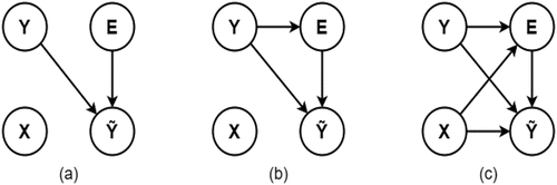
In Figure 1, Y represents the true labels, E represents the possibility of occurrence of an error, X represents the input feature vector and $\tilde{y}$ represents the predicted output. From the figure, we can see that occurrence of a NCAR type of label noise is not dependent on the other variables, including the true labels itself with an error probability of $P_e=P\left(E=1\right)=P\left(Y\ne \tilde{y}\right)$ where the incorrectness in the label is chosen at random (Frenay and Verleysen 2013; Angluin and Laird 1988). In the case of NAR, the possibility of error in labels is dependent on the true label while the error probability is $P_e=P\left(E=1\right)=\hspace{0.17em}\sum _{y\in Y}P\left(Y=y\right)P(E=1|Y=y)$ (Frenay and Verleysen 2013). NNAR is the most realistic case of noise as the source of noise can both be the input images and the label images (Algan and Ulusoy 2020). This representation of label noise is the most complex label noise relation with the probability of error which follows the equation, $P_e\left(x,y\right)=P\left(E=1|X=x,Y=y\right)$ (Frenay and Verleysen 2013).

Extraordinary improvement of deep learning methods has created more advanced and efficient techniques for different computer vision tasks over the last decade (Khamparia and Mehtab Singh 2019). However, obstacles like label noise still need to be dealt with as it is an inseparable part of modern computer vision. Many researchers found that deep learning models can put up with noise up to a certain level (Algan and Ulusoy 2020; Rolnick et al. 2017). Go¨rkem Algan and Ilkay Ulusoy showed that feature dependent label noise which is a NAR type of label noise, affects the model’s performance by reducing the test accuracy (Algana and Ulusoy 2021). Another study showed that the more the presence of label noise, the more the accuracy is reduced in the case of satellite image classification, but the proper distribution of high-intensity noise into the study area tends to increase the correctness of the model (Boonprong et al. 2018).

Deep Neural Networks for Image Segmentation

A rapid paradigm shift was seen in the deep learning paradigm when the ImageNet model outperformed all other state-of-the-art techniques in the ImageNet LSVRC-2010 contest (Alex, Sutskever, and Hinton 2017). In the following years, varying deep learning techniques and approaches for innumerable use cases were discovered by researchers. The use of different deep learning approaches bought significant improvement in the segmentation task with remarkable performance (Garcia-Garcia et al. 2017). As the progression of deep learning thrived over the last decade, the convolutional neural network (CNN) has performed admirably in many computer vision tasks (Voulodimos et al. 2018). However, image segmentation has been one of the most difficult tasks in computer vision for the previous three decades (Wurm et al. 2019). Image segmentation holds a major position in the domain of computer vision for its further implications in many other sectors. Crucial sectors like medical (Nima et al. 2020; Olaf, Fischer, and Brox 2015), geospatial data analysis (Liu et al. 2018), and autonomous driving (Sharma et al. 2019) uses segmentation technique as a solution to several other implementations.

Application of recent findings in semantic image segmentation (Yanming et al. 2018) has yielded some encouraging results in terms of accuracy and performance. Furthermore, advanced Convolutional Neural Network models have resulted in significant improvements over previous semantic segmentation methods (Long, Shelhamer, and Darrell 2015; Ming et al. 2019). Cas-FCN, a less sophisticated but high-performing model for ultrasound maternity image segmentation which has been proposed (Ming et al. 2019). (Long, Shelhamer, and Darrell 2015) developed a segmentation architecture that includes fully convolutional models such as AlexNet, GoogleNet, and VGG. For enhanced feature extraction, their study used a combination of upsampling technique and patch-wise training mechanisms, as well as skip connections, which are employed across the layers to fuse coarse. Despite the fact that deep learning works effectively for segmentation tasks, vanishing gradient and overfitting are still issues when training deep neural networks (Evgin 2019).

Complex images are difficult to segment because information localized in images poses difficulty for the model to understand. Satellite images, for example, are a collection of compressed high-level data that can be difficult to segment. More advanced deep learning models, such as UNet (Khryashchev et al. 2019) and DeepLabV3 (Chen et al. 2017), come in helpful here. For the optimum feature extraction, UNet is an FCNN (Fully Connected Neural Network) that uses skip connections between the ‘contracting’ and ‘expansive’ components of the network (Olaf, Fischer, and Brox 2015). The medical sector has seen the most impactful deployment of U-Net-based segmentation models so far (Garcia-Garcia et al. 2017; Nima et al. 2020). This architecture has been used for chronic stroke lesion segmentation (Liu et al. 2018), retina-vessel segmentation (Robert and Shapiro 1985), nuclei segmentation in histology images (Olaf, Fischer, and Brox 2015), liver and tumor segmentation (Garcia-Garcia et al. 2017), and investigating heart-conditions from ultrasound images (echo-cardiography) (Naz, Majeed, and Irshad 2010).

The positive impact of U-net-like architecture in the medical field prompted numerous researchers to investigate its usage in other circumstances where segmentation is advantageous and required in some cases. Though it was originally designed for medical image segmentation, UNet has been used for a variety of other applications, including sea-land segmentation (Chu et al. 2019), street tree segmentation (Junjun et al. 2020), satellite image segmentation (Khryashchev et al. 2019), sediment segmentation (Pranto et al. 2021), tomato leaf segmentation (C. Ngugi, Abdelwahab, and Abo-Zahhad 2020), real-time hair segmentation (Yoon, Park, and Yoo 2021), hand segmentation in complex background (Wang, Wang, and Juan 2011), pedestrian segmentation (Nurhadiyatna and Lončarić 2017), etc. We extended our previous study (Pranto et al. 2021) on sedimentation segmentation and analyzed three different label noise on the performance of segmentation model and the model performance under different magnitude and volume of these noises.

Study Area

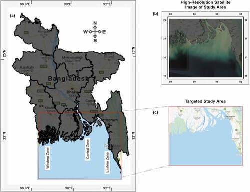
Bangladesh’s marine territory is separated into three zones (Belal 2012): the coastal marine region (12 nautical miles), the exclusive economic zone (200 nautical miles), and the seabed off the coast (350 nautical miles). These marine regions conjointly occupy an area of 165,887 square kilometers. The geographic coordinate of the Bangladesh marine region is at the latitude and longitude of 20.99°N, 90.73°E (Marine Gazetteer Placedetails 2020). Our frame of reference for this study is located at (89.09, 20.37) in the South-West, (92.34, 20.37) in the South-East, (92.34, 22.91) in the North-East, and (89.09, 22.91) in the North-West, which is located at the lower stream to many rivers, which creates a large load of sedimentation in the Bay of Bengal’s estuary. The study area is divided into three parts based on geographic features, the eastern zone, central zone, and western zone, among which the central zone is considered to the most susceptible to sediment load as river Meghna falls into this region which is a major contributor of sedimentation (Ahmad 2019). Our study area has been depicted in Figure 2.

Figure 2. (a) Bangladesh geographical location. (b) High-resolution satellite image of target Region. (c) Targeted marine region.

Data Extraction and Preparation

Labeling and Extracting Satellite Images in GEE

For the purpose of image extraction, we used Copernicus Sentinel-2 satellite and images at 10 m resolution were used in our study. The rectangular area is located at (89.09, 20.37) in South-West, (92.34, 20.37) in the South-East, (92.34, 22.91) in North-East, and (89.09, 22.91) in North-West is our reference frame for clipping images. We also collected the images of four separate time frames, which are January–February 2020, November–December 2019, January–February 2019, and November–December 2018. The whole process of image labeling and extraction is shown in the figure below (Figure 3). More details of the process could be found elsewhere (Pranto et al. 2021).

Figure 3. Image labeling and band extraction (a) 12-band satellite image. (b) Labeling with google earth engine. (c) Generating shapefile by QGis Software. (d) Adding shapefile as the 13^th band to the original image.

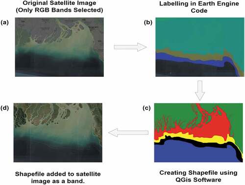
Collecting images from satellites and making them compatible with deep learning algorithms required several steps of data perpetration and pre-processing. For that purpose, we used Google Earth Engine (GEE), which provides a compact package of various tools and functionalities. First of all, we extracted image tiles of our target area. From several image tiles of a particular location, we filtered out the best possible tile using different filtration mechanisms provided by the GEE JavaScript API. Using the in-built filtration tools of GEE, we selected tiles that had cloud cover less than 1%, and we also checked if the image tile passed geometric, radiometric and sensor tests of GEE. Only these selected tiles were used to form our original image. After the selection of tiles has been made, for labeling the image tiles, we used the GEE polynomial tool. Using the polynomial tool, we can define the categorical class of a labeled region. For our study, we have five classes, among which we labeled four classes in GEE and the remaining portion is the fifth class. After finishing the labeling, we collected the labeled images to further process them in QGIS software. The target area is erroneous in size and for that reason, the total area is composed of several disjointed image tiles which need to be joined as well as the labeling which falls out of the target area also needs to be clipped from the original area of interest. We used QGIS for these tasks and the final resultant shapefile was our mask that needed to be added to the original images. We added this labeled image as the fourth band of our original image, which made the original image a four-band image where the first three bands (RGB) compose the input image and the fourth band is the mask for our segmentation model.

Data Preparation

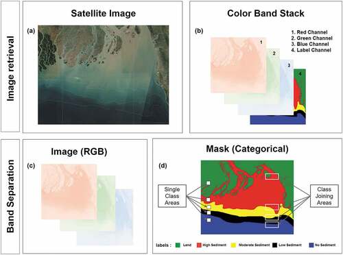
Deep learning models are not compatible with huge satellite image tiles. Comparatively smaller labeled images can be used directly, but in our case, the image size was 36141 × 28197 units at 10 m resolution. For making images usable to the deep learning algorithm, first, we separated the label (4th band) from the original image which is our mask images for the segmentation model. Then, image and mask were cropped into 15762 patches using the python GDAL library where each patch was measured 256 × 256 pixels in height and width. Both images and masks contain two kinds of regions that the model has to distinguish which is shown in Figure 4(b). Moreover, these images are often affected by values that are hard to be dealt with (e.g., infinite values, ‘Nan’ values). These values do not cause any error while reading the images but affect the error metrics substantially. These kinds of concealed flaws are hard to find which caused us great difficulty to fine-tune the model’s performance. ‘Nan’ values were replaced by the nearest class labels in our study. The process of image-mask separation and patch cropping is shown in the figure below (Figure 4).

Figure 4. Preparing dataset from the satellite image. (a) 4-band satellite image (4^th band is a label). (b) Stacked layers of an image. (c) The first three layers (bands) are separated as the image. (d) 4^th band is separated as a mask.

Methodology: Modification U-Net Architecture

The left part of the U-Net design (Olaf, Fischer, and Brox 2015) is called the contracting part, and the right part is called the expansive part. Juxtaposing these two parts forms a shape identical to “U” which reflects on the model’s architecture. We used the same form of architecture with modification in the shapes across the model while sub-dividing the model into 11 groups for easier explanation. The Rectified linear unit (ReLU) activation is used between the layers and the output layer uses a SoftMax activation function. The model is divided into two parts and a combination of these two parts together segments an input image. The model architecture is shown in the figure below (Figure 5).

Figure 5. Modified U-Net architecture used in this study.

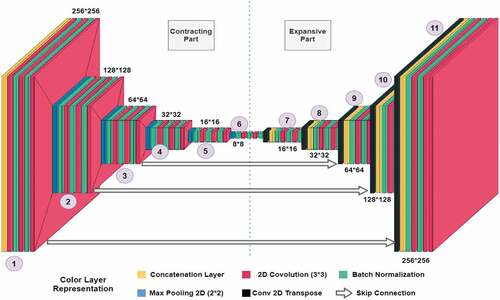
Contracting Part

The stack indicated as 1 in Figure 5 takes 256 × 256 images as input. This layer is constructed of concatenating layers which precede a layer of unpadded 2d-convolution with 64, (3*3) kernels, followed by batch normalization with 2*2 kernel, stride size of 2, and momentum of 0.01. The second and third stacks are identical in the architecture. Values are copied or sent to the expanded portion of the model through skip connection at this step. The picture is then shrunk to 128*128 by passing it through a 2d-max-polling layer with kernel size (2*2) and stride 2. Group 3ʹs layer layout is identical to that of group 2. The layer configuration in groups 4,5 and 6 is identical to that in group 2, with the exception that there is no skip connection in these layers.

Expansive Part

The model’s expansive component begins with group 7. A Conv2d-transpose layer with 64 kernels of size (3*3) and stride of 2 is used to start a group in the expansive section. This layer does the inverse of 2d-Convolution. This is followed by a concatenation layer, batch normalization, and a 2d-convolution layer. This pattern is repeated until the 11th group, and the final layer picture has a form of 256*256*5.

Evaluation Metrics and Loss Function

Dice Coefficient

The dice coefficient is a statistic for evaluating segmentation performance of. It quantifies the proportion of similarity between the real image and the image predicted by the model (Tustison and Gee 2009). Equation 1(1) $DiceCoefficient=\frac{2\ast intersection\left(A\ast B\right)}{\left(A+B\right)}$(1) represents the formula of dice coefficient where A is the true image and the predicted image is denoted as B.

(1) $DiceCoefficient=\frac{2\ast intersection\left(A\ast B\right)}{\left(A+B\right)}$(1)

Categorical Cross-Entropy

Categorical Cross-entropy, often known as negative log loss function, is often used as a loss calculation metric to multi-class classification problems (Yaoshiang and Wookey 2019). For real image representation $y$ and predicted image representation $\hat{y}$, the loss is calculated using equation 2(2) $\mathrm{L}\left(y,\hat{y}\right)=\sum _{j=0}^M\sum _{i=0}^N\left(y_{ij}\ast log\left(\hat{y}\right)\right)$(2) .

(2) $\mathrm{L}\left(y,\hat{y}\right)=\sum _{j=0}^M\sum _{i=0}^N\left(y_{ij}\ast log\left(\hat{y}\right)\right)$(2)

SoftMax

SoftMax activation determines the difference between two vectorized one-hot encoded probability distributions and examines the probability of a pixel belonging to a particular class (Nwankpa et al. 2018). The task of semantic segmentation requires classification of each class, hence, calls for pixel-wise SoftMax to each pixel. The softMax activation function is expressed as following equation 3(3) $\sigma \left({\vec{z}}_i\right)=\frac{e^{z_i}}{\sum _{k=1}^n{e}^{z_k}}$(3) .

(3) $\sigma \left({\vec{z}}_i\right)=\frac{e^{z_i}}{\sum _{k=1}^n{e}^{z_k}}$(3)

The normal exponential function is represented by e, the input vector is represented by z, and the number of classes is represented by n in equation 3(3) $\sigma \left({\vec{z}}_i\right)=\frac{e^{z_i}}{\sum _{k=1}^n{e}^{z_k}}$(3) .

Pixelwise Accuracy

Pixel accuracy holds profound importance in semantic segmentation. Pixel accuracy refers to the percentage of pixels successfully classified (percentage of true positive rate) by the segmentation algorithm (Wang, Wang, and Zhu 2020). True-positive is represented as TP and false-positive as FP, and the equation of pixel accuracy is shown in equation 4(4) $PixelAccuracy=\frac{{\sum }_{n}T{P}_n}{{\sum }_n(T{P}_n+F{P}_n)}$(4) .

(4) $PixelAccuracy=\frac{{\sum }_{n}T{P}_n}{{\sum }_n(T{P}_n+F{P}_n)}$(4)

Result and Analysis

We have analyzed the results and predictions of our model from two perspectives, with and without noisy labels. In the satellite image, noise is a common phenomenon (Asokan and Anitha 2020) where, on the other hand, labeling by human experts also increases the amount of noise (Frenay and Verleysen 2013) as different human being labels an image from their own confidence (deciding upon the label). We have tested our best-performing model, that is, Dec2019, under three kinds of label noise.

In extension to our previous work (Pranto et al. 2021), we conducted a comprehensive study on label noise in this study. The best image over a region is taken on when the satellite is in its NADIR position (Zhou et al. 2020) (satellite perpendicular to a point on earth). The off-NADIR position creates an angle between the sensor of the satellite and the region. Moreover, sunlight also has an angle of reflectance over a region in which satellite image is being taken. So, analysis of the model’s robustness under different levels of rotation and flip has been analyzed in this study. On the other hand, salt and paper (Lopes et al. 2020) is another common noise seen in satellite images. So, we also experimented with complete random noise, which represents salt and pepper noise.

Analysis of Result under Noiseless Labels

During the model training, 70% of the data was utilized for training, while the remaining 30% was used for testing. For 30 epochs, the models were trained. This criterion was applied to each of the four datasets. Figures 6 and 7 illustrate the change in training and validation dice co-efficient and training and validation loss over 30 epochs, respectively.

Figure 6. Dice coefficient during training and validation over 30 epochs.

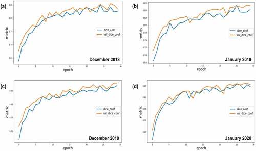
Figure 7. Loss during training and validation over 30 epochs.

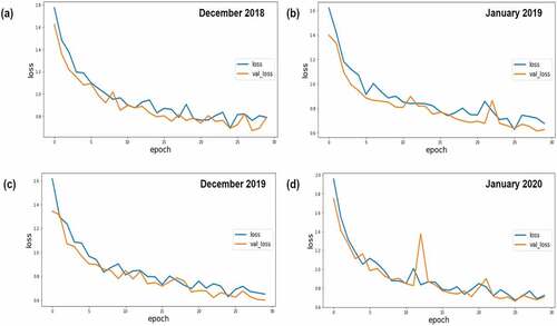
The model looks to be learning some pattern in the data based on the pixel accuracy, loss, and dice coefficient values and graphs. The loss is smoothly dropping in accordance with the validation loss, while the dice coefficient follows the same pattern. As for dice coefficient as a performance evaluation metric, the models appear to perform well, with the greatest co-efficient of 85% for both training and validation. The images contain two types of areas, one with one of the five classes and the other with two independent classes joining. Our experiment considers both these cases to determine the predictive capability of the model. The Dice coefficient, loss and pixel-wise accuracy scores have been shown in Table 1.

Table 1. Performance measurement for four-year dataset.

	Dice coefficient (%)	Validation dice coefficient (%)	Loss	Validation loss	Validation loss (%)	Validation pixel accuracy (%)
December 2018	85.51	85.42	0.695	0.667	74.88	73.34
January 2019	86.72	86.76	0.627	0.614	77.47	77.07
December 2019	86.86	87.81	0.628	0.600	77.00	78.97
January 2020	85.76	86.22	0.672	0.661	75.25	75.83

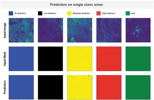
The next two consecutive figures below show the prediction of our model for class join regions (Figure 8) as well as for single class regions (Figure 9).

Figure 8. Prediction on regions with two class.

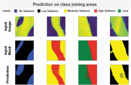
Figure 9. Prediction on regions with one class.

Analysis of Result under Label Noise

In the previous section, we saw how the models perform for different year datasets under noiseless labels. The same model performed almost similarly for all these datasets, but the Dec-2019 model comparatively performed better than the other datasets. In this section, we will present the result and metric as well as model predictions for our best-performing model.

NCAR – Noise Completely at Random

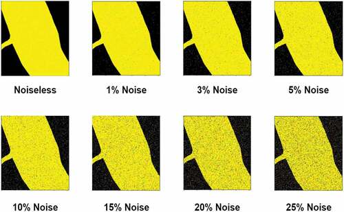
The noise completely at random appears completely randomly and class independently. In our study, each pixel in an image belongs to one of the five classes as follows: Class 0: Land, class1: high-sediment, class 2: moderate sedimentation, class 3: low sedimentation, and class 4: water/no-sedimentation. We randomly chose x% of the pixels and randomly altered the class to any of the other classes creating completely random noise. For instance, 5% NCAR noise injection means every training image will have 5% of its pixels intentionally miss-classed. We injected random noise in the range of 1% to 25%. The percentage we chose are 1,3,5,10,15,20 & 25%. The figure below (Figure 10) shows the gradual increase of complete random label noise.

Figure 10. Example of complete random label noise in a range from 1% to 25%.

The table below (Table 2) shows the metric and accuracy measurements of the model under different percentages of complete random noise.

Table 2. Dice coefficient, pixel accuracy, and loss for complete random label noise.

Noise (%)	Dice coefficient (%)	Validation dice coefficient (%)	Loss	Validation loss	Pixel accuracy (%)	Validation pixel accuracy (%)
1%	87.51	87.42	0.595	0.607	78.88	78.34
3%	85.02	86.15	0.734	0.703	74.99	76.44
5%	83.94	85.33	0.796	0.752	72.16	75.11
10%	82.85	83.94	0.874	0.843	71.48	73.35
15%	81.14	81.70	0.954	0.952	69.07	69.40
20%	79.18	79.76	1.03	1.02	65.11	65.85
25%	78.65	79.20	1.07	1.05	64.11	65.21

From the table (Table 2), we can clearly see that, as we increase the percentage of completely random label noise, the model’s performance seems to drop. Where the dice coefficient for 1% noise was 87.51% and pixel accuracy was 78.88%, for 25% label noise, dice coefficient drops to 78.65% and pixel accuracy drops to 64.11%. The same scenario is seen in the case of loss. From 0.595 for 1% completely random noise, loss increases to 1.07 for 25% complete random noise. The following figure (Figure 11) shows prediction on class join regions under different percentages of completely random label noise.

Figure 11. Class-join prediction under complete random label noise.

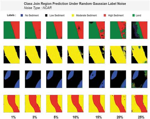
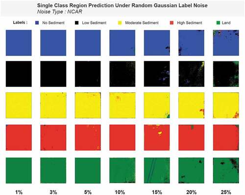
The figure shows that the model performs almost similarly to noiseless models up until 10% noise. After that, a slight drop is seen for 15% noise. But, as we get closer to the highest noise, that is 25%, performance changes drastically. The same characteristic of performance drop is also seen in predictions of single class region areas (Figure 12).

Figure 12. Single-class region prediction under random Gaussian label noise.

NAR – Rotation with Nearest Fill Mode Label Noise

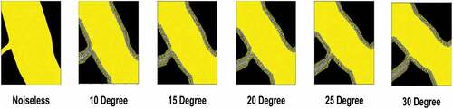
Rotation is a type of random noise but not completely at random. An image can only be rotated at a certain angle which is not entirely random. Our approach to rotation is slightly different; labels were rotated between 10^◦ to 30^◦ with an interval of 5^◦, and the gap created due to rotation was filled with the “Nearest” mode of the python SciPy library to avoid artificial pixel filling. The figure below (Figure 13) contains some examples of rotation with nearest fill noise.

Figure 13. Example of rotational label noise (10^◦ to 40^◦) with nearest fill mode.

The next two figures (Figure 14,15) show the model’s prediction capability under different levels of rotational noise.

Figure 14. Class-join region prediction under rotational label noise.

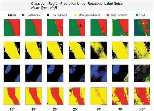
Figure 15. Single class prediction under rotational noise ranging from 10^◦ to 30^◦.

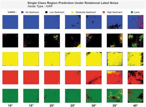
The figures depict that up to 20^◦ rotations; the model predicts almost similar to the noiseless model while more rotation than 20^◦ rotation causes performance drop. From the metric-accuracy table (Table 3), we can also see that rotation more than 20^◦ brings down both pixel accuracy and dice coefficient drastically. The prediction image also shows the same characteristic as we can clearly see the model guessing randomly both for a single class and class join regions. The table below (Table 3) contains the accuracy and metrics of model performance under rotation noise.

Table 3. Dice coefficient, pixel accuracy, and loss for rotational label noise.

Rotation	Dice coefficient (%)	Validation dice coefficient (%)	Loss	Validation loss	Pixel accuracy (%)	Validation pixel accuracy (%)
10◦	88.46	87.54	0.562	0.610	80.78	78.21
15◦	87.53	87.65	0.616	0.613	79.09	79.01
20◦	85.43	86.76	0.705	0.649	74.49	77.14
25◦	80.78	81.14	0.717	0.726	72.28	71.84
30◦	71.23	73.26	0.958	0.918	67.35	68.16

As we can see from the table (Table 3), as we increase rotation performance of the model de- creases notably. Dice coefficient of 88.46% for 10^◦ rotation reduces down to 71.23% for 30^◦ rotations. Same type of scenario is seen in the case of validation dice coefficient. On the other hand, loss of 0.562 for 10^◦ rotations increases up to 0.95 for 30^◦ of rotations. These values of evaluation metrics clearly depict that up to 20^◦, the models show robust nature against noise but rotation more than 20^◦ drops performance significantly.

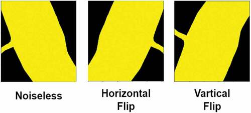
NNAR – Label Flip Noise

In label flip noise, we flipped the labels vertically and horizontally. This is an NNAR (noise not at random) type of noise. The figure below (Figure 16) shows an example of label flip noise on a mask image.

Figure 16. Example of horizontal and vertical flip label noise.

The next two figures below (Figure 17,18) show the prediction of our deep neural model under label flip noise.

Figure 17. Class-join region prediction under horizontal and vertical flip label noise.

Figure 18. Single-class region prediction under horizontal and vertical flip label noise.

We can see in Figures 17 and Figure 18 that, under label flip, the model’s performance is considerably poor. The model for some labels cannot segment properly, let alone a clean segmentation. For both horizontal and vertical flip, the model seems to lose its segmentation capability. This intuition seeing the prediction images can be further justified using metrics, loss and accuracy table. The table below (Table 4) shows the pixel accuracy and metrics results under horizontal and vertical label flip noise.

Table 4. Dice coefficient, pixel accuracy, and loss for label flip noise.

Flip	Dice coefficient (%)	Validation dice coefficient (%)	Loss	Validation loss	Pixel accuracy (%)	Validation pixel accuracy (%)
Horizontal	65.94	63.83	1.365	1.647	61.50	63.23
Vertical	67.53	64.65	1.416	1.513	63.09	62.01

Table 4 shows that, for label flip, U-Net does not perform well for segmentation tasks. The loss is high and accuracy and dice coefficient is considerably low which leads the model to random guesses for pixels. The next two images show the model’s performance under label flip noise for both class-join regions and single class regions.

Discussion

In this study, we investigated how a semantic segmentation model behaves under different intensities of label noise. We specifically worked with label noise because satellite image data is generally extracted using filtration techniques which removes feature noises in the earliest stage. But, during labeling, human experts or crowd-sourced labeling are often noisy. This impairs the model’s learning and also eventually hurts the performance of the model. From our experimentation, we found that an increasing amount of NCAR noise gradually decreases the model’s performance. Until 20^◦ rotation (NAR noise), the U-Net model yields competitive performance and rotation greater than 20^◦ is intolerable by the segmentation model. Whereas on the other hand, flipping the labels completely puzzles the model and performance drops drastically where the model seems to produce random predictions. All these three noises were injected into the training images based on their intensity while the original masks being noise-free. After training, the result was generated using noise-free test sets.

Conclusion

Noise is an inseparable part of satellite images data. Understanding noise thus aids the purpose of building robust solutions to specific problems under label noise. Without a proper understanding of how a deep learning segmentation model can react to different kinds of noises, it is difficult to build precise solutions. In this study, we conducted an in-depth analysis of the performance of deep learning model under three prevalent kinds of noise (NCAR – noise completely at random, NAR – noise at random and NNAR – noise not at random) that can be present in the labels. For complete random label noise, which is a NCAR type of noise, seven magnitudes of noise percentage were used. As we increase the percentage of complete random noise, Dice Coefficient falls, loss increases, and pixel-wise accuracy drops at an equidistant trend compared to the previous value of each other. There is no sudden dramatic change in these values. However, for rotation noise, which is a NAR type of noise the trend is different. Up to 20^◦, the model Dice Coefficient stays above 85% and drops in an equidistant trend. But after 20^◦, rotation, a sudden downfall of every parameter is observed. For NNAR, horizontal or vertical flip of noise shows a significant negative impact on the performance. Dice Coefficient drops in the vicinity of 65% and pixel-wise accuracy to 62%, which leads the model to random guess. Although noise imparts the performance of segmentation, augmentation is a strong means of improving model performance via providing more data. Augmentation uses different noise-like techniques to generate new data. Using remotely sensed satellite data is a cost-effective way to investigate and analyze sedimentation in the marine area without reaching into the study field while wasting valuable time and resources. For the future work of this study, we have the desire to work with the de-lineation of sediment in the marine region of Bangladesh as well as in the river banks. Our implementation has been made generic enough that can aid the other similar works. For encouraging future research, our implementation has been made public and can be found at https://github.com/Tahmid1406/Sediment-Load-Performance-Under-Label-Noise.

Acknowledgments

This work is supported by Faculty Research Grant (CTRG-20-SEPS-14), North South University, Bashundhara, Dhaka 1229, Bangladesh.

Disclosure statement

No potential conflict of interest was reported by the authors.

References

- Ahmad, H. 2019. Bangladesh coastal zone management status and future trends. Journal of Coastal Zone Management 22 (1):1–2453.
- Alex, K., I. Sutskever, and G. E. Hinton. 2017. ImageNet classification with deep convolutional neural networks. Communications of the ACM (ACM New York, NY, USA) 60(6):84–90. doi:10.1145/3065386.
- Algan, G., and İ. Ulusoy. 2020. “Label noise types and their effects on deep learning.” arXiv preprint arXiv:2003.10471.
- Algana, G., and I. Ulusoy. 2021. Image classification with deep learning in the presence of noisy labels: A survey. Knowledge-Based Systems (Elsevier) 215:106771. doi:10.1016/j.knosys.2021.106771.
- Angluin, D., and P. Laird. 1988. Learning from noisy examples. Machine Learning (Springer) 2(4):343–70. doi:10.1023/A:1022873112823.
- Asokan, A., and J. Anitha. 2020. Adaptive Cuckoo search based optimal bilateral filtering for denoising of satellite images. ISA Transactions (Elsevier) 100:308–21. doi:10.1016/j.isatra.2019.11.008.
- Belal, A. S. M. 2012. Maritime boundary of Bangladesh: Is Our Sea Lost? Bangladesh Institute of Peace and Security Studies. https://www.files.ethz.ch/isn/164392/mb_bd.pdf
- Boonprong, S., C. Cao, W. Chen, N. Xiliang, X. Min, and B. Kumar Acharya. 2018. The classification of noise-afflicted remotely sensed data using three machine-learning techniques: Effect of different levels and types of noise on accuracy. ISPRS International Journal of Geo-Information (Multidisciplinary Digital Publishing Institute) 7 (7):274. doi:10.3390/ijgi7070274.
- Borra, S., R. Hanki, and N. Dey. 2019. Satellite image enhancement and analysis. In Satellite image analysis: clustering and classification, ed. Janusz Kacprzyk,13–29. Singapore: Springer. doi:10.1007/978-981-13-6424-2_2.
- BWDB. 2021. Bangladesh Water Development Board | On Going Project. January. Accessed January 11, 2021. https://www.bwdb.gov.bd/rivers-information.
- C. Ngugi, L., M. Abdelwahab, and M. Abo-Zahhad. 2020. Tomato leaf segmentation algorithms for mobile phone applications using deep learning. Computers and Electronics in Agriculture (Elsevier) 178:105788. doi:10.1016/j.compag.2020.105788.
- CEGIS. 2021. Comprehensive Resource Database. Accessed February 03, 2021. https://www.cegisbd.com/cegis/Home.aspx.
- Chen, L.-C., G. Papandreou, F. Schroff, and H. Adam. 2017. “Rethinking atrous convolution for semantic image segmentation.” arXiv:1706.05587.
- Chouhan, S. S., A. Kaul, and U. Pratap Singh. 2018. Soft computing approaches for image segmentation: A survey. Multimedia Tools and Applications (Springer) 77 (21):28483–537. doi:10.1007/s11042-018-6005-6.
- Chu, Z., T. Tian, R. Feng, and L. Wang. 2019. “Sea-land segmentation with res-UNet and fully connected CRF.” IGARSS 2019-2019 IEEE International Geoscience and Remote Sensing Symposium. Yokohama, Japan: IEEE. 3840–43. doi:10.1109/IGARSS.2019.8900625.
- Cui, B., X. Chen, and L. Yan. 2020. Semantic segmentation of remote sensing images using transfer learning and deep convolutional neural network with dense connection. IEEE Access (IEEE) 8:116744–55. doi:10.1109/ACCESS.2020.3003914.
- Ericson, J. P., J. Charles, S. Vörösmarty, L. Dingman, L. G. Ward, and M. Meybeckc. 2006. Effective sea-level rise and deltas: Causes of change and human dimension implications. Global and Planetary Change (Elsevier) 50 (1–2):63–82. doi:10.1016/j.gloplacha.2005.07.004.
- Evgin, G. 2019. “Challenges and recent solutions for image segmentation in the era of deep learning.” 2019 Ninth International Conference on Image Processing Theory, Tools and Applications (IPTA). Istanbul, Turkey: IEEE. 1–6. doi:10.1109/IPTA.2019.8936087.
- Frenay, B., and M. Verleysen. 2013. Classification in the presence of label noise: A survey. IEEE Transactions on Neural Networks and Learning Systems (IEEE) 25 (5):845–69. doi:10.1109/TNNLS.2013.2292894.
- Garcia-Garcia, A., S. Orts-Escolano, S. Oprea, V. Villena-Martinez, and J. Garcia-Rodriguez. 2017. “A review on deep learning techniques applied to semantic segmentation.” arXiv preprint arXiv:1704.06857.
- Hussain, M. G., A. A. K. Pierre Failler, M. Khurshed Alam, and M. K. Alam. 2018. Major opportunities of blue economy development in Bangladesh. Journal of the Indian Ocean Region (Taylor &Francis) (1) 14:88–99. doi:10.1080/19480881.2017.1368250.
- Islam, M. M., and M. Shamsuddoha. 2018. Coastal and marine conservation strategy for Bangladesh in the context of achieving blue growth and sustainable development goals (SDGs). Environmental Science & Policy (Elsevier) 87:45–54. doi:10.1016/j.envsci.2018.05.014.
- Junjun, L., J. Cao, M. Ebissa Feyissa, and X. Yang. 2020. Automatic building detection from very high-resolution images using multiscale morphological attribute profiles. Remote Sensing Letters (Taylor & Francis) 11(7):640–49. doi:10.1080/2150704X.2020.1750729.
- Khamparia, A., and K. Mehtab Singh. 2019. A systematic review on deep learning architectures and applications. Expert Systems (Wiley Online Library) 36(3):e12400. doi:10.1111/exsy.12400.
- Khryashchev, V., R. Larionov, A. Ostrovskaya, and A. Semenov. 2019. “Modification of U-Net neural network in the task of multichannel satellite images segmentation.” 2019 IEEE East-West Design & Test Symposium (EWDTS). Batumi, Georgia: IEEE. 1–4. doi:10.1109/EWDTS.2019.8884452.
- Lei, M., Y. Liu, X. Zhang, Y. Yuanxin, G. Yin, and B. Alan Johnson. 2019. Deep learning in remote sensing applications: A meta-analysis and review. ISPRS Journal of Photogrammetry and Remote Sensing (Elsevier) 152:166–77. doi:10.1016/j.isprsjprs.2019.04.015.
- Liu, Y., Q. Ren, J. Geng, M. Ding, and L. Jiangyun. 2018. Efficient patch-wise semantic segmentation for large-scale remote sensing images. Sensors (Multidisciplinary Digital Publishing Institute) 18 (10):3232. doi:10.3390/s18103232.
- Long, J., E. Shelhamer, and T. Darrell. 2015. “Fully convolutional networks for semantic segmentation.” 2015 IEEE Conference on Computer Vision and Pattern Recognition (CVPR). Boston, MA, USA: IEEE. 3431–40. doi:10.1109/CVPR.2015.7298965.
- Lopes, M., P.-L. Frison, M. Crowson, E. Warren-Thomas, B. Hariyadi, W. D. Kartika, F. Agus, K. C. Hamer, L. Stringer, J. K. Hill, et al. 2020. Improving the accuracy of land cover classification in cloud persistent areas using optical and radar satellite image time series. Methods in Ecology and Evolution (Wiley Online Library) 11(4):532–41. doi:10.1111/2041-210X.13359.
- Marine Gazetteer Placedetails. Accessed January 20, 2020. https://www.marineregions.org/gazetteer.php?p=details&id=25431.
- Ming, W., C. Zhang, J. Liu, L. Zhou, and L. Xiaoqi. 2019. Towards accurate high resolution satellite image semantic segmentation. IEEE Access (IEEE) 7:55609–19. doi:10.1109/ACCESS.2019.2913442.
- Naz, S., H. Majeed, and H. Irshad. 2010. “Image segmentation using fuzzy clustering: A survey.” 2010 6th International Conference on Emerging Technologies (ICET). Islamabad, Pakistan: IEEE. 181–86. doi:10.1109/ICET.2010.5638492.
- Nima, T., L. Jeyaseelan, L. Qian, J. N. Chiang, W. Zhihao, and X. Ding. 2020. Embracing imperfect datasets: A review of deep learning solutions for medical image segmentation. Medical Image Analysis (Elsevier) 63:101693. doi:10.1016/j.media.2020.101693.
- Nurhadiyatna, A., and S. Lončarić. 2017. “Semantic image segmentation for pedestrian detection.” Proceedings of the 10th International Symposium on Image and Signal Processing and Analysis. Ljubljana, Slovenia: IEEE. 153–58. doi:10.1109/ISPA.2017.8073587.
- Nwankpa, C., W. Ijomah, A. Gachagan, and S. Marshall. 2018. “Activation functions: Comparison of trends in practice and research for deep Learning.” arXiv preprint arXiv:1811.03378.
- O’Shea, K., and R. Nash. 2015. “An introduction to convolutional neural networks.” arXiv preprint arXiv:1511.08458.
- Olaf, R., P. Fischer, and T. Brox. 2015. MICCAI: International Conference on Medical Image Computing and Computer-Assisted Intervention, October 5-9, Munich, Germany. In Edited by J. Hornegger, W. M. Wells, and A. F. F. N. Navab, vol. 9351, 234–41. Springer. doi:10.1007/978-3-319-24574-4_28.
- Panboonyuen, T., K. Jitkajornwanich, S. Lawawirojwong, P. Srestasathiern, and P. Vateekul. 2019. Semantic segmentation on remotely sensed images using an enhanced global convolutional network with channel attention and domain specific transfer learning. Remote Sensing (Multidisciplinary Digital Publishing Institute) 11 (1):83. doi:10.3390/rs11010083.
- Pranto, T. H., A. All Noman, A. Noor, U. Habiba Deepty, and R. M. Rahman. 2021. Patch-wise semantic segmentation of sedimentation from high-resolution satellite images using deep learning. Vol. 12861, in International Work-Conference on Artificial Neural Networks (IWANN, 2021) part of Lecture Notes in Computer Science, by Ignacio Rojas, Andreu Catala and Gonzalo Joya, 498–509. Springer, Cham. doi:10.1007/978-3-030-85030-2_41.
- Robert, M. H., and L. G. Shapiro. 1985. Image segmentation techniques. Computer Vision, Graphics, and Image Processing (Elsevier) 29 (1):100–32. doi:10.1016/S0734-189X(85)90153-7.
- Rolnick, D., A. Veit, S. Belongie, and N. Shavit. 2017. “Deep learning is robust to massive label noise.” arXiv preprint arXiv:1705.10694.
- Sharma, S., J. E. Ball, B. Tang, D. W. Carruth, M. Doude, and M. Aminul Islam. 2019. Semantic segmentation with transfer learning for Off-Road autonomous driving. Sensors (Multidisciplinary Digital Publishing Institute) 19 (11):2577. doi:10.3390/s19112577.
- Singh, P., and R. Shree. 2016. “Analysis and effects of speckle noise in SAR images.” 2016 2nd International Conference on Advances in Computing, Communication, & Automation (ICACCA)(Fall). Bareilly, India: IEEE. 1–5. doi:10.1109/ICACCAF.2016.7748978.
- Talukdar, S., P. Singha, S. Mahato, S. Swades Pal, Y.-A. Liou, A. Rahman, and A. Rahman. 2020. Land-use land-cover classification by machine learning classifiers for satellite observations—A review. Remote Sensing (Multidisciplinary Digital Publishing Institute) 12 (7):1135. doi:10.3390/rs12071135.
- Tustison, N., and J. C. Gee. 2009. Introducing Dice, Jaccard, and other label overlap measures to ITK. The Insight Journal. doi:10.54294/1vixgg.
- Voulodimos, A., N. Doulamis, A. Doulamis, and E. Protopapadakis. 2018. Deep learning for computer vision: A brief review. Computational Intelligence and Neuroscience (Hindawi) 2018:1–13. doi:10.1155/2018/7068349.
- Wang, X.-Y., T. Wang, and B. Juan. 2011. Color image segmentation using pixel wise support vector machine classification. Pattern Recognition (Elsevier) 44 (4):777–87. doi:10.1016/j.patcog.2010.08.008.
- Wang, Z., E. Wang, and Y. Zhu. 2020. Image segmentation evaluation: A survey of methods. Artificial Intelligence Review (Springer) 53 (8):5637–74. doi:10.1007/s10462-020-09830-9.
- Wurm, M., T. Stark, X. Xiang Zhu, M. Weigand, and H. Taubenböck. 2019. Semantic segmentation of slums in satellite images using transfer learning on fully convolutional neural networks. ISPRS Journal of Photogrammetry and Remote Sensing (Elsevier) 150:59–69. doi:10.1016/j.isprsjprs.2019.02.006.
- Xiao, P., Y. Guo, and P. Zhuang. 2018. Removing stripe noise from infrared cloud images via deep convolutional networks. IEEE Photonics Journal (IEEE) 10 (4):1–14. doi:10.1109/JPHOT.2018.2854303.
- Yang, C., C. Zhang, L. Qingquan, H. Liu, W. Gao, T. Shi, X. Liu, and W. Guofeng. 2020. Rapid urbanization and policy variation greatly drive ecological quality evolution in Guangdong-Hong Kong-Macau Greater Bay Area of China: A remote sensing perspective. Ecological Indicators 115:106373. doi:10.1016/j.ecolind.2020.106373.
- Yanming, G., Y. Liu, T. Georgiou, and M. S. Lew. 2018. A review of semantic segmentation using deep neural networks. International Journal of Multimedia Information Retrieval 7 (2):87–93. doi:10.1007/s13735-017-0141-z.
- Yaoshiang, H., and S. Wookey. 2019. The real-world-weight cross-entropy loss function: Modeling the costs of mislabeling. IEEE Access (IEEE) 8:4806–13. doi:10.1109/ACCESS.2019.2962617.
- Yoon, H.-S., S.-W. Park, and J.-H. Yoo. 2021. Real-time hair segmentation using mobile-Unet. Electronics (MDPI) 10(2):99. doi:10.3390/electronics10020099.
- Zeyu, X., Z. Shen, L. Yang, L. Xia, H. Wang, L. Shuo, S. Jiao, and Y. Lei. 2021. Road extraction in mountainous regions from high-resolution images based on DSDNet and terrain optimization. Remote Sensing (Multidisciplinary Digital Publishing Institute) 13 (1):90. doi:10.3390/rs13010090.
- Zhou, Q., L. Tian, L. Jian, W. Hua, and Q. Zeng. 2020. Radiometric cross-calibration of large-view-angle satellite sensors using global searching to reduce BRDF influence. IEEE Transactions on Geoscience and Remote Sensing (IEEE) 59 (6):5234–45. doi:10.1109/TGRS.2020.3019969.