A Fully Bayesian Inference with Gibbs Sampling for Finite and Infinite Discrete Exponential Mixture Models

ABSTRACT

In this paper, we propose clustering algorithms based on finite mixture and infinite mixture models of exponential approximation to the Multinomial Generalized Dirichlet (EMGD), Multinomial Beta-Liouville (EMBL) and Multinomial Shifted-Scaled Dirichlet (EMSSD) with Bayesian inference. The finite mixtures have already shown superior performance in real data sets clustering using the Expectation–Maximization approach. The proposed approaches in this paper are based on a Monte Carlo simulation technique namely Gibbs sampling algorithm including an additional Metropolis–Hastings step, and we utilize exponential family conjugate prior information to construct their posterior relying on Bayesian theory. Furthermore, we also present the infinite models based on Dirichlet processes, which results in clustering algorithms that do not require the specification of the number of mixture components to be given in advance and selects it in a principled manner. The performance of our Bayesian approaches was evaluated in some challenging real-world applications concerning text sentiment analysis, fake news detection, and human face gender recognition.

Introduction

Clustering count vectors is a challenging task on large data sets considering its high dimensionality and sparsity nature (Jain 2010). The bag of words representation for text systematically exhibits the burstiness phenomenon, if a word appears once in a document, it is much more likely to appear again (Church and Gale 1995; Katz 1996). This phenomenon is not limited to text and can also be observed in images with visual words (Jegou, Douze, and Schmid 2009).

Table 1. Experiment results for IMDB movie reviews.

Method	Precision	Recall	F-Measure
FinEMBL-MCMC	$84.72\pm 0.1$	$87.88\pm 0.07$	$86.27\pm 0.05$
FinEMGD-MCMC	$85.16\pm 0.05$	$88.73\pm 0.03$	$87.03\pm 0.04$
FinEMSSD-MCMC	$86.14\pm 0.07$	$83.84\pm 0.04$	$84.96\pm 0.07$
InfEMBL-MCMC	$89.18\pm 0.09$	$88.93\pm 0.07$	$89.06\pm 0.06$
InfEMGD-MCMC	$88.68\pm 0.03$	$88.49\pm 0.04$	$88.58\pm 0.06$
InfEMSSD-MCMC	$\mathbf{88}\mathbf{.57}\pm \mathbf{0}\mathbf{.05}$	$\mathbf{89}\mathbf{.60}\pm \mathbf{0}\mathbf{.07}$	$\mathbf{89}\mathbf{.08}\pm \mathbf{0}\mathbf{.05}$
EMGD-EM	$81.36\pm 0.10$	$85.55\pm 0.11$	$83.59\pm 0.09$
EMBL-EM	$83.75\pm 0.12$	$84.60\pm 0.13$	$84.17\pm 0.10$
EMSSD-EM	$82.96\pm 0.11$	$83.01\pm 0.12$	$82.98\pm 0.10$

Table 2. Experiment results for Tripadvisor hotel reviews.

Method	Precision	Recall	F-Measure
FinEMBL-MCMC	$70.23\pm 0.05$	$70.31\pm 0.10$	$70.16\pm 0.12$
FinEMGD-MCMC	$69.94\pm 0.01$	$69.88\pm 0.08$	$69.84\pm 0.16$
FinEMSSD-MCMC	$74.37\pm 0.17$	$74.45\pm 0.04$	$74.32\pm 0.23$
InfEMBL-MCMC	$70.36\pm 0.09$	$70.43\pm 0.07$	$70.31\pm 0.06$
InfEMGD-MCMC	$70.39\pm 0.13$	$70.47\pm 0.34$	$70.34\pm 0.26$
InfEMSSD-MCMC	$\mathbf{74}\mathbf{.67}\pm \mathbf{0}\mathbf{.15}$	$\mathbf{74}\mathbf{.76}\pm \mathbf{0}\mathbf{.13}$	$\mathbf{74}\mathbf{.58}\pm \mathbf{0}\mathbf{.09}$
EMGD-EM	$67.50\pm 0.17$	$69.48\pm 0.15$	$68.48\pm 0.12$
EMBL-EM	$66.73\pm 0.17$	$70.68\pm 0.16$	$68.65\pm 0.13$
EMSSD-EM	$73.39\pm 0.15$	$73.39\pm 0.14$	$73.39\pm 0.14$

It also has a sparsity nature that few words show up with high occurrence and some are less as often as possible or do not appear at all (Margaritis and Thrun 2001). Thus, such data are generally represented as sparse high-dimensional vectors, with few thousands of dimensions with a sparsity of 95–99% (Dhillon and Modha 2001).

Hierarchical Bayesian modeling frameworks, such as Generalized Dirichlet multinomial mixture model (GDM), Beta-Liouville multinomial mixture model (MBL) and Shifted-Scaled Dirichlet multinomial mixture model (MSSD) (Alsuroji, Zamzami, and Bouguila 2018; Bouguila 2008; Elkan 2006), have shown excellent performance for high-dimensional count data clustering. However, their estimation procedures are very inefficient when the data collection size is large (Zamzami and Bouguila 2020a). The exponential family of distributions has a finite-sized sufficient statistics (Brown 1986), meaning that we can compress the data into a fixed-sized summary without loss of information (DasGupta 2011). Efficient exponential family approximations to the MGD (EMGD), MBL (EMBL) and MSSD (EMSSD) have been previously proposed by Zamzami and Bouguila (Zamzami and Bouguila 2020a, 2022, 2020b). These distributions have shown to address the burstiness phenomenon successfully and to be considerably computationally faster than their original distribution forms especially when dealing with sparse and high-dimensional data (i.e. these exponential approximations are evaluated as functions or non-zero counts only as we will see in the next section).

The main problem in the case of finite mixture models is the estimation of the model parameters (Brooks 2001). Expectation–maximization (EM) algorithm is a simple and effective approach for model’s parameters estimation (Emanuel and Herman 1987). However, the EM algorithm for finite mixtures has several drawbacks. For example, the occurrence of local maximum and singularities in likelihood function will often cause problems for deterministic gradients method (Robert 2007). Moreover, in high dimensional estimation, it will be hard to obtain reliable estimates which possess generalization capabilities to predict the densities at new data points (Cai 2010; Dias and Wedel 2004). Some Bayesian approaches are based on simulation methods, such as Gibbs sampling, which explore high-density regions (Roeder and Wasserman 1997). The stochastic aspect of these simulation methods ensures the escape from local maximum (e.g., Bouguila, Ziou, and Hammoud 2009). Tsionas (2004) proposed an estimation approach for multivariate t distribution using Gibbs sampling with data augmentation. Amirkhani, Manouchehri, and Bouguila (2021) presented a fully Bayesian approach within Monte Carlo simulation for Multivariate Beta mixture parameters estimation. Bouguila, Ziou, and Hammoud (2009) successfully adopted a Bayesian algorithm based on Metropolis-within Gibbs sampling for a finite Generalized Dirichlet mixture. Najar, Zamzami, and Bouguila (2019) used Monte Carlo simulation method for exponential family approximation to the Dirichlet Compound Multinomial mixture model (EDCM) parameters estimation and shown excellent results in some real applications. Xuanbo, Bouguila, and Zamzami (2021) successfully proposed a fully Bayesian approach based on Gibbs sampling technique for exponential family approximation to the Multinomial Scaled Dirichlet mixture model (EMSD).

Another challenging aspect when using finite mixture model is usually to estimate the number of clusters which best describes the data without overfitting or underfitting it. For this purpose, many approaches have been suggested. These approaches can be divided into two different strategies for mixture models. The first strategy is the implementation of model selection criteria. The second strategy is resampling from the full posterior distribution with the number of clusters considered unknown. However, the majority of these approaches cannot be easily used for high-dimensional data (Bouguila and Ziou 2010). The infinite mixture models based on Dirichlet process (Antoniak 1974; Korwar and Hollander 1973) have recently attracted wide attention, thanks to the development of MCMC techniques. Dirichlet process mixture (DPM) models resolve the difficulties related to model selection (MacEachern and Muller 1998). Rasmussen (1999) successfully applied Dirichlet process on Gaussian mixture model with Gibbs sampling to obtain accurate number of classes. Bouguila and Ziou (2010) also presented a clustering algorithm for Dirichlet process mixture of Generalized Dirichlet distributions with MCMC techniques. Najar, Zamzami, and Bouguila (2020) proposed an infinite mixture of exponential family approximation to the Multinomial Dirichlet Compound mixture model and showed superior experimental results in recognition of human interactions in feature films. Thus, we extend these finite mixture models to infinite mixture models based on Dirichlet process to tackle model selection in the case of sparse high-dimensional vectors.

In this paper, we present clustering algorithms based on finite and infinite mixtures of EMGD, EMBL and EMMSD from Bayesian viewpoint using Gibbs sampling within M–H steps. These distributions have already shown excellent performances in clustering real-world high-dimensional count data sets with deterministic approach. The key contributions of this article are as following: (1) Determination of conjugate priors to EMGD, EMBL and EMSSD by taking into account the fact that these distributions are members of the exponential family, and (2) through challenging applications that concern text sentiment analysis, text fake news detection and human face gender recognition, we show that the proposed algorithms are efficient for clustering sparse high-dimensional count data. The learning of the proposed finite mixtures and their infinite counterparts will be based on MCMC algorithms namely Gibbs sampling and Metropolis–Hastings (M–H) (Favaro and Whye Teh 2013).

The rest of this paper is organized as follows. The next two sections, review and develop conjugate prior distributions for the EMBL, EMGD and EMSSD distributions. Then, we present a Bayesian estimation for their finite mixture models parameters using Gibbs sampling, and extend these finite mixture models to infinite mixture models while developing complete clustering algorithms. After we exhibit the abilities of the proposed approaches in text sentiment analysis, text fake news detection, human face gender recognition. The concluding remarks and future work directions are given at the end of the paper.

Exponential Approximation of Distributions for Count Data

In this section, we review the approximations to the MGD, the MBL and the MSSD to bring them to the exponential family of distributions.

Exponential Family

The exponential family of distributions is widely used in machine learning research due to its sufficient property, as the sufficient statistics can give all of needed parameter information by the whole sample data set. For a random variable $X$ and a distribution with $M$ parameters in exponential family we have:

(1) $p(X|\xi )\propto H(X)exp(\sum _{l=1}^M{G}_l(\xi ))T_l(X)+\mathrm{\Phi }(\xi ))$(1)

where $G_l(\xi )$ is called the natural parameter, $T_l$ (X) is the sufficient statistic, $H(X)$ is the underlying measure, and $\mathrm{\Phi }(\xi )$ is called log normalizer used to ensure that the distribution integrates to one (DasGupta 2011).

The Exponential Family Approximation to Multinomial Generalized Dirichlet (MGD) Distribution

We define $X=(x_1,\cdots ,x_{D+1})$ as a sparse count data vector describing a text document, or an image where $x_d$ corresponds to the frequency of appearances of a word or visual word $w$. The MGD distribution is defined by (Bouguila 2008):

(2) $MGD(X|\xi )=\frac{\mathrm{\Gamma }(n+1)}{{\prod }_{d=1:x_d\ge 1}^{D+1}\mathrm{\Gamma }(x_d+1)}\prod _{d=1:x_d\ge 1}^D\frac{\mathrm{\Gamma }({\alpha }_d+{\beta }_d)}{\mathrm{\Gamma }({\alpha }_d)\mathrm{\Gamma }({\beta }_d)}\frac{\mathrm{\Gamma }({\alpha }_d^{\mathrm{\prime }}+{\beta }_d^{\mathrm{\prime }})}{\mathrm{\Gamma }({\alpha }_d^{\mathrm{\prime }})\mathrm{\Gamma }({\beta }_d^{\mathrm{\prime }})}$(2)

where $n={\sum }_d^{D+1}{x}_d$, ${\alpha }^{\mathrm{\prime }}={\alpha }_d+x_d$, ${\beta }^{\mathrm{\prime }}={\beta }_d+x_{d+1}\cdots +x_{D+1}$, for $d=1,\cdots ,D$, and $\xi =(\alpha ,\beta )$. In count data represented as bag-of-words, Zamzami and Bouguila (2020a) found, experimentally, that ${\alpha }_d\ll {\beta }_d\ll 1$ for almost all words $w$ based on different data sets. Moreover, we have for $x\ge 1$ (Elkan 2006):

(3) $\underset{\alpha \to 0}{lim}\frac{\mathrm{\Gamma }(\alpha +x)}{\mathrm{\Gamma }(\alpha )}-\alpha \mathrm{\Gamma }(x)=0$(3)

Then, the exponential family form for MGD can be written as (Zamzami and Bouguila 2022):

(4) $\begin{array}{c}EMGD(X|\xi )\propto (\prod _{D:x_D\ge 1}{x}_d^{-1})\prod _{D:x_D\ge 1}\frac{\mathrm{\Gamma }(z_d)}{\mathrm{\Gamma }(x_d+z_d)}n\times \{exp\sum _{d=1}^{D}I(x_d>=1)log\frac{{\alpha }_d{\beta }_d}{{\alpha }_d+{\beta }_d}\}\end{array}$(4)

where $I(x_d>=1)$ is an indicator that represents whether a word $w$ shows up at any entry in the vector $X$, and $z_d=x_{d+1}+\cdots +x_{D+1}$.

The Exponential-Family Approximation to Multinomial Beta-Liouville (MBL) Distribution

If a random vector $X=(x_1,\cdots ,x_{D+1})$ follows a Multinomial Beta-Liouville distribution, then (Bouguila 2011):

(5) $MBL(X|\xi )=\frac{\mathrm{\Gamma }(({\sum }_{d=1}^{D+1}{x}_d)+1)}{{\prod }_{d=1}^{D+1}\mathrm{\Gamma }(x_d+1)}\times \frac{\mathrm{\Gamma }({\sum }_{d=1}^D{\alpha }_d)\mathrm{\Gamma }(\alpha +\beta )\mathrm{\Gamma }({\alpha }^{\mathrm{\prime }})\mathrm{\Gamma }({\beta }^{\mathrm{\prime }}){\prod }_{d=1}^D\mathrm{\Gamma }({\alpha }_d^{\mathrm{\prime }})}{\mathrm{\Gamma }({\sum }_{d=1}^D{\alpha }_d^{\mathrm{\prime }})\mathrm{\Gamma }({\alpha }^{\mathrm{\prime }}+{\beta }^{\mathrm{\prime }})\mathrm{\Gamma }(\alpha )\mathrm{\Gamma }(\beta ){\prod }_{d=1}^D\mathrm{\Gamma }({\alpha }_d)}$(5)

where ${\alpha }_d^{\mathrm{\prime }}={\alpha }_d+x_d$, ${\alpha }^{\mathrm{\prime }}=\alpha +{\sum }_{d=1}^D{x}_d$, ${\beta }^{\mathrm{\prime }}=\beta +x_{D+1}$, and $\xi =(\alpha ,\beta )$.

In several real world applications, the MBL mixture model has provided good high clustering accuracy, comparably to Multinomial Scaled Dirichlet mixture model (MSD) (Zamzami and Bouguila 2019), and Multinomial Generalized Dirichlet mixture model (MGD) (Bouguila 2008), it also outperforms other widely used mixture models, such as mixtures of Multinomial distributions (MM) and Dirichlet Compound Multinomial (DCM) distributions (Bouguila and Ziou 2007; Madsen, Kauchak, and Elkan 2005). However, MBL does not belong to the exponential family, and it is not efficient in high-dimensional spaces where many parameters need to be estimated (Zamzami and Bouguila 2020a). Approximating MBL to belong to exponential family can reduce the computation cost and improve the efficiency of MBL to model sparse high-dimensional count data (Elkan 2006).

Zamzami and Bouguila (2020a) found empirically that $\alpha \ll 1$ and $\beta \simeq 1$ for real data sets and proposed maximum likelihood method for model parameters estimation. Thus, relying on Equation (3)(3) $\underset{\alpha \to 0}{lim}\frac{\mathrm{\Gamma }(\alpha +x)}{\mathrm{\Gamma }(\alpha )}-\alpha \mathrm{\Gamma }(x)=0$(3) , we have the form of exponential approximation for multinomial Beta-Liouville distribution as:

(6) $EMBL(X|\xi )\propto (\prod _{d:x_d>=1}{x}_d^{-1})n!\frac{\mathrm{\Gamma }(S)\mathrm{\Gamma }({\alpha }^{\mathrm{\prime }})\mathrm{\Gamma }({\beta }^{\mathrm{\prime }})\alpha }{\mathrm{\Gamma }(S+n)\mathrm{\Gamma }({\alpha }^{\mathrm{\prime }}+{\beta }^{\mathrm{\prime }})}exp\{\sum _{d=1}^{D}I(x_d\le 1)log({\alpha }_d)\}$(6)

where $I(x_d>=1)$, the sufficient static, is an indicator whether the word $d$ appears at least once in the vector $X$ and $S={\sum }_{d=1}^D{\alpha }_d$.

2.4. The Exponential-Family Approximation to Shifted Scaled Dirichlet Multinomial (MSSD) Distribution

Define a random vector $X=(x_d,\cdots ,x_D)$ that follows a Shifted Scaled Dirichlet Multinomial Distribution, then:

(7) $MSSD(X|\xi )\approx \frac{n!\mathrm{\Gamma }({\alpha }_{+})}{\prod _{d:x_d\ge 1}^D{x}_d!\mathrm{\Gamma }({\alpha }_{+}\tau N)}\prod _{d:x_d\ge 1}^D\frac{\mathrm{\Gamma }({\alpha }_d+\tau x_d)}{{\beta }_d^{x_d}\mathrm{\Gamma }({\alpha }_d)}$(7)

where ${\alpha }_{+}={\sum }_d^D{\alpha }_d$, $n={\sum }_{d=1}^D{x}_d!$ and $\xi =(\alpha ,\beta ,\tau )$.

For high dimensional data, Zamzami and Bouguila (2020b) found that the value of $\alpha$ parameters are really small which combined with some approximations gave the exponential Multinormial Shifted-Scaled Dirichlet (EMSSD) as:

(8) $EMSSD(X|\xi )\propto n!\frac{\mathrm{\Gamma }({\alpha }_{+}){\tau }^D}{\mathrm{\Gamma }({\alpha }_{+}+\tau N)}\prod _{d:x_d\ge 1}^D\frac{\alpha }{{\beta }_d^{x_d}{x}_d\tau }$(8)

The Proposed Bayesian Learning Framework

In this section, we propose the algorithms to learn the parameters for finite and infinite mixture models of EMBL, EMGD and EMMSD.

Finite Mixture of Distributions

A finite mixture of distributions with $M$ components is defined as (e.g., (Bouguila and Fan 2020)):

(9) $P(X|\xi )=\sum _{j=1}^{M}p(X|{\xi }_j)P_j$(9)

where the $P_j$ are the mixing weights and $p(X|{\xi }_j)$ is the components distribution, $\mathrm{\Theta }=(\xi ,P)$ is the entire set of parameters to be estimated, where $\xi =({\xi }_1\cdots {\xi }_M)$, ${\xi }_j$ represents the parameters of distribution $j$, and $P=(P_1,\cdots ,P_M)$ is the vector of weight parameters. The $P_j$ must satisfy: $0\le P_j\le 1,j=1\cdots M,{\sum }_{j=1}^M{P}_j=1$.

Bayesian Learning for Finite Mixture Weight Parameters

Given a set of $N$ independent vectors $\mathcal{X}=(X_1\cdots X_N)$ described by a finite mixture model, and $M$ is the number of mixture components, supposed to be known, the main problem is to estimate the mixture parameters. In this work, we rely on Bayesian techniques to resolve this problem.

We define an indicator for each $X_i$ in data set $\mathcal{X}$ for each class $j$ as:

(10) $Z_{ij}=\left\{\begin{array}{ccc}\hspace{0.17em}& 1& if{X}_{i}belongstoclassj\\ \hspace{0.17em}& 0& otherwise\end{array}\right.$(10)

where $\mathbf{Z}=\{Z_1,\cdots ,Z_N\}$ and $Z_i=(Z_{i1},\cdots ,Z_{iM})$. In the Bayesian paradigm information brought by the complete data ($\mathcal{X},\mathbf{Z}$), a realization of ($\mathcal{X},\mathbf{Z}$) $\sim p(\mathcal{X},\mathbf{Z}|\mathrm{\Theta })$ is combined with prior information about the parameters $\mathrm{\Theta }$ that is specified in a prior distribution with density $\pi (\mathrm{\Theta })$ and summarized in probability distribution $\pi (\theta |\mathcal{X},\mathbf{Z})$ called the posterior distribution. This can be derived from the joint distribution, $p(\mathcal{X},\mathbf{Z}|\mathrm{\Theta })\pi (\theta )$ (Nizar, Ziou, and Hammoud 2009). Thus, we have:

(11) $\begin{array}{ccc}\pi (\xi |\mathcal{X},\mathbf{Z})& =\frac{\pi (\xi )p(\mathcal{X},\mathbf{Z}|\xi )}{\int \pi (\xi )p(\mathcal{X},\mathbf{Z}|\xi )d\xi }& \propto \pi (\xi )\times p(\mathcal{X},\mathbf{Z}|\xi )\end{array}$(11)

where $\int \pi (\xi )p(\mathcal{X},\mathbf{Z}|\xi )d\xi$ is the marginal density of the complete data $(\mathcal{X},\mathbf{Z})$. We can directly simulate $\xi \sim \pi (\xi |\mathcal{X},\mathbf{Z})$ with well-known Gibbs sampler rather than directly computing it. Gibbs sampling is widely used in Bayesian mixture model, especially in the case of incomplete data (Train 2009; Xuanbo, Bouguila, and Zamzami 2021). That is, associate with each observation $X_i$ a missing multinomial variable $\mathbf{Z}\sim \mathbf{M}(1,{\hat{Z}}_{i1},\cdots ,{\hat{Z}}_{iM})$.

(12) ${\hat{Z}}_{ij}=\frac{p(X_j|\xi )P_j}{{\sum }_{j=1}^{M}p(X_j|\xi )P_j}$(12)

In fact, the weight parameter is independent of $\mathcal{X}$, $P\propto \pi (P|\mathbf{Z})$ (Samuel, Balakrishnan, and Johnson 2000), and we know that the vector $P$ is defined on the simplex {($P_1,\cdots ,P_M);{\sum }_{j=1}^{M-1}{P}_j<1$}, then the natural prior distribution for vector $P$ is the Dirichlet distribution, we determine the prior of $P$ (Lee 2012) as:

(13) $\pi (P|\eta )=\frac{\mathrm{\Gamma }({\sum }_{j=1}^M{\eta }_j)}{{\prod }_{j=1}^M\mathrm{\Gamma }({\eta }_j)}\prod _{j=1}^M{P}_j^{{\eta }_j-1}$(13)

where $\eta =({\eta }_1,\cdots ,{\eta }_M)$ is the parameters vector of the Dirichlet distribution. Moreover, we have:

(14) $\begin{array}{c}\pi (\mathbf{Z}|P)=\prod _{i=1}^N\pi (Z_i|P)=\prod _{i=1}^N{P}_1^{Z_{i1}}\cdots P_M^{Z_{iM}}=\prod _{i=1}^N\prod _{j=1}^M{P}_j^{Z_{ij}}=\prod _{j=1}^M{P}_j^{n_j}\end{array}$(14)

where $n_j={\sum }_{i=1}^N{I}_{Z_{ij}=1}$, Having the prior distribution and likelihood distribution in hand, we can obtain the posterior for weight parameters $P$ by the following:

(15) $\begin{array}{cc}\pi (P|\mathbf{Z})& \propto \pi (P)\pi (\mathbf{Z}|P)\\ \hspace{0.17em}& =\prod _{j=1}^M{P}_j^{n_j}\frac{\mathrm{\Gamma }(\sum _{j=1}^M{\eta }_j)}{{\prod }_{j=1}^M\mathrm{\Gamma }({\eta }_j)}\prod _{j=1}^M{P}_j^{{\eta }_j-1}\\ \hspace{0.17em}& =\frac{\mathrm{\Gamma }({\sum }_{j=1}^M{\eta }_j)}{{\prod }_{j=1}^M\mathrm{\Gamma }({\eta }_j)}\prod _{j=1}^M{P}_j^{{\eta }_j+n_j-1}\\ \hspace{0.17em}& \propto D({\eta }_1+n_1\cdots {\eta }_M+n_M)\end{array}$(15)

where $D$ is Dirichlet distribution with parameters $({\eta }_1+n_1,\cdots ,{\eta }_M+n_M)$. We note that the prior and posterior distributions $\pi (P)$ and $\pi (P|\mathbf{Z})$ are both Dirichlet distributions. In this case, we say that the Dirichlet is conjugate prior for mixture proportions. Therefore, the weight parameters can be sampled from Dirichlet distribution. We selected ${\eta }_j=1,j=1,\dots ,M$ in our experiments.

The Bayesian Learning for Infinite Mixture Weight Parameters

In finite mixture model, we have considered $M$ to be fixed finite quantity. In this section, we will explore the limit $M\to \mathrm{\infty }$ and present the conditional posteriors for the indicators and weight parameters based on Dirichlet process. We take $({\eta }_1,\cdots ,{\eta }_M)=(\eta /M,\cdots ,\eta /M)$ for Equation (11)(11) $\begin{array}{ccc}\pi (\xi |\mathcal{X},\mathbf{Z})& =\frac{\pi (\xi )p(\mathcal{X},\mathbf{Z}|\xi )}{\int \pi (\xi )p(\mathcal{X},\mathbf{Z}|\xi )d\xi }& \propto \pi (\xi )\times p(\mathcal{X},\mathbf{Z}|\xi )\end{array}$(11) , thus we obtain a simpler form for prior probability of infinite mixture weight parameters:

(16) $\pi (P_{inf}|\eta )=\frac{\mathrm{\Gamma }(\eta )}{\mathrm{\Gamma }{(\eta /M)}^M}\prod _{j=1}^M{\pi }_j^{\eta /M-1}$(16)

where we have $P_{inf}=(P_{in{f}^1},\cdots ,P_{in{f}^M})$. From Equation (12)(12) ${\hat{Z}}_{ij}=\frac{p(X_j|\xi )P_j}{{\sum }_{j=1}^{M}p(X_j|\xi )P_j}$(12) , we have the prior distribution for the Z parameter that corresponds to multinomial distribution. Using the standard Dirichlet integral, we could marginalize out the $P_{inf}$ parameter to get the following probability for the prior directly in terms of the indicators (Rasmussen 1999):

(17) $\begin{array}{cc}p(\mathbf{Z}|\eta )& =\int P(\mathbf{Z}|P_{inf})P(P_{inf}|\eta )\\ \hspace{0.17em}& =\frac{\mathrm{\Gamma }(\eta )}{\mathrm{\Gamma }{(\eta /M)}^M}\int \prod _{j=1}^M{\pi }^{n_j+\eta /M-1}d{\pi }_j\\ \hspace{0.17em}& =\frac{\mathrm{\Gamma }(\eta )}{\mathrm{\Gamma }(N+\eta )}\prod _{j=1}^M\frac{\mathrm{\Gamma }(n_j+\eta /M)}{\mathrm{\Gamma }(\eta /M)}\end{array}$(17)

Based on Bayes principle, we obtain the conditional posterior distribution for the mixing weight vector:

(18) $\begin{array}{cc}\pi (P_{inf}|\mathbf{Z})& =\frac{p(P_{inf}|\eta )p(\mathbf{Z}|P_{inf})}{p(\mathbf{Z}|\eta )}\\ \hspace{0.17em}& =\prod _{j=1}^M{P}_{in{f}^j}^{n_j}\frac{\mathrm{\Gamma }({\sum }_{j=1}^M\eta )}{{\prod }_{j=1}^M\mathrm{\Gamma }({\eta }_j)}\prod _{j=1}^M{P}_{in{f}^j}^{\eta /M-1}\\ \hspace{0.17em}& =\frac{\mathrm{\Gamma }({\sum }_{j=1}^M\eta /M)}{{\prod }_{j=1}^M\mathrm{\Gamma }(\eta /M)}\prod _{j=1}^M{P}_{in{f}^j}^{\eta /M+n_j-1}\\ \hspace{0.17em}& \propto D(\eta /M+n_1\cdots \eta /M+n_M)\end{array}$(18)

In order to be able to use Gibbs sampling for the indicators $Z_i$, we need the conditional prior for a single indicator given all the others: this is easily obtained from Equation (17)(17) $\begin{array}{cc}p(\mathbf{Z}|\eta )& =\int P(\mathbf{Z}|P_{inf})P(P_{inf}|\eta )\\ \hspace{0.17em}& =\frac{\mathrm{\Gamma }(\eta )}{\mathrm{\Gamma }{(\eta /M)}^M}\int \prod _{j=1}^M{\pi }^{n_j+\eta /M-1}d{\pi }_j\\ \hspace{0.17em}& =\frac{\mathrm{\Gamma }(\eta )}{\mathrm{\Gamma }(N+\eta )}\prod _{j=1}^M\frac{\mathrm{\Gamma }(n_j+\eta /M)}{\mathrm{\Gamma }(\eta /M)}\end{array}$(17) by keeping all but a single indicator fixed (Najar, Zamzami, and Bouguila 2020):

(19) $p(Z_i=j|Z_{\mathrm{\_}}i,\eta )=\frac{n_{\mathrm{\_}i,j}+\eta /M}{N-1+\eta }$(19)

where the subscript $-i$ indicates all except $i$ and $n_{\mathrm{\_}i,j}$ is the number of observations, excluding $X_i$, that are associated with component $j$.

Lastly, we choose inverse Gamma as prior for parameters $\eta$:

(20) $\begin{array}{c}p(\eta |\vartheta ,\rho )=\frac{{\rho }^{\vartheta }exp(-\rho /\eta )}{\mathrm{\Gamma }(\vartheta ){\eta }^{\vartheta +1}}\end{array}$(20)

The likelihood for $\eta$ can be derived from Equation (17)(17) $\begin{array}{cc}p(\mathbf{Z}|\eta )& =\int P(\mathbf{Z}|P_{inf})P(P_{inf}|\eta )\\ \hspace{0.17em}& =\frac{\mathrm{\Gamma }(\eta )}{\mathrm{\Gamma }{(\eta /M)}^M}\int \prod _{j=1}^M{\pi }^{n_j+\eta /M-1}d{\pi }_j\\ \hspace{0.17em}& =\frac{\mathrm{\Gamma }(\eta )}{\mathrm{\Gamma }(N+\eta )}\prod _{j=1}^M\frac{\mathrm{\Gamma }(n_j+\eta /M)}{\mathrm{\Gamma }(\eta /M)}\end{array}$(17) , which together with the prior from Equation (19)(19) $p(Z_i=j|Z_{\mathrm{\_}}i,\eta )=\frac{n_{\mathrm{\_}i,j}+\eta /M}{N-1+\eta }$(19) gives:

(21) $p(\eta |\vartheta ,\rho ,M,N)=\frac{{\rho }^{\vartheta }exp(-\rho /\eta )}{\mathrm{\Gamma }(\vartheta ){\eta }^{\vartheta +1}}\times \frac{{\eta }^M\mathrm{\Gamma }(\eta )}{\mathrm{\Gamma }(N+\eta )}$(21)

We selected $(\vartheta ,\rho )=(4,2)$ in our experiments. These values were previously used in Bouguila and Ziou (2010), because they allow a diffuse range of values of the number of clusters $M$ (more details and discussions can be found in Escobar and West 1995). For the indicators, letting $M\to \mathrm{\infty }$ in Equation (19)(19) $p(Z_i=j|Z_{\mathrm{\_}}i,\eta )=\frac{n_{\mathrm{\_}i,j}+\eta /M}{N-1+\eta }$(19) , the conditional prior reaches the following limits (Rasmussen 1999):

(22) $p(Z_i=j|\eta ,Z_{\mathrm{\_}i})=\left\{\begin{array}{ccc}\hspace{0.17em}& \frac{n_{\mathrm{\_}i,j}}{N-1+\eta }& if{n}_{\mathrm{\_}ij}>0\\ \hspace{0.17em}& \frac{\eta }{N-1+\eta }& if{n}_{\mathrm{\_}ij}=0\\ \hspace{0.17em}& \hspace{0.17em}& \hspace{0.17em}\end{array}\right.$(22)

Having this prior distribution, we can obtain the conditional posterior by multiplying the model likelihood:

(23) $p(Z_i=j|\eta ,Z_{\mathrm{\_}i})=\left\{\begin{array}{ccc}\hspace{0.17em}& \frac{n_{\mathrm{\_}i,j}}{N-1+\eta }p(\mathcal{X}|\xi )& if{n}_{\mathrm{\_}ij}>0\\ \hspace{0.17em}& \int \frac{\eta }{N-1+\eta }p(\mathcal{X}|\xi )p(\xi )d\xi & if{n}_{\mathrm{\_}ij}=0\\ \hspace{0.17em}& \hspace{0.17em}& \hspace{0.17em}\end{array}\right.$(23)

Unfortunately, this integral is not analytically tractable in Equation (23)(23) $p(Z_i=j|\eta ,Z_{\mathrm{\_}i})=\left\{\begin{array}{ccc}\hspace{0.17em}& \frac{n_{\mathrm{\_}i,j}}{N-1+\eta }p(\mathcal{X}|\xi )& if{n}_{\mathrm{\_}ij}>0\\ \hspace{0.17em}& \int \frac{\eta }{N-1+\eta }p(\mathcal{X}|\xi )p(\xi )d\xi & if{n}_{\mathrm{\_}ij}=0\\ \hspace{0.17em}& \hspace{0.17em}& \hspace{0.17em}\end{array}\right.$(23) , hence, we consider a Monte Carlo sampling approximation.

Learning Algorithm for Finite Mixture Model of EMGD

Define $\pi (\xi )$ as the prior distribution for the parameters of the EMGD distribution. We use the fact that EMGD belongs to the exponential family. In fact, if a S-parameters density $\rho$ belongs to the exponential family then we can rewrite it in the exponential form which has been shown in Equation (1)(1) $p(X|\xi )\propto H(X)exp(\sum _{l=1}^M{G}_l(\xi ))T_l(X)+\mathrm{\Phi }(\xi ))$(1) .

Writing the EMGD in the exponential form gives:

(24) $\begin{array}{cc}H(X)& =(\prod _{W:x_W\ge 1}{x}_w^{-1})\prod _{W:x_W\ge 1}\frac{\mathrm{\Gamma }(z_w)}{\mathrm{\Gamma }(x_w+z_w)}n!\\ G_w(\xi )& =log\frac{{\alpha }_w{\beta }_w}{{\alpha }_w+{\beta }_w}\\ T_w(X)& =\sum _{w=1}^{W}I(x_w>=1)\\ \varphi (\xi )& =0\\ \hspace{0.17em}& \hspace{0.17em}\end{array}$(24)

In this case, a prior of $\xi$ is given by (Lee 2012) as:

(25) $\pi (\xi )\propto exp(\sum _{w=1}^W{\rho }_l{G}_w(\xi )+k\mathrm{\Phi }(\xi ))$(25)

where $\rho =({\rho }_1,\cdots ,{\rho }_w)$, and $k>0$ are referred as hyperparameters.

The prior for EMGD can be written as following:

(26) $\pi (\alpha ,\beta )\propto exp(\sum _{w=1}^W{\rho }_{l}log\frac{{\alpha }_w{\beta }_w}{{\alpha }_w+{\beta }_w})$(26)

Having the prior in hand, the mixture model posterior is (see Appendix A):

(27) $\begin{array}{cc}\pi ({\xi }_j|\mathbf{M},\mathbf{X})& \propto \pi ({\xi }_j)\prod _{Z_{ij}=1}EMGD(X_i|{\xi }_j)\\ \hspace{0.17em}& \propto exp[\sum _{w=1}^{W}log\frac{{\alpha }_w{\beta }_w}{{\alpha }_w+{\beta }_w}({\rho }_w+\sum _{Z_{ij}=1}^{N}I(x_{iw}\ge 1))]\\ \hspace{0.17em}& \times \prod _{Z_{ij}=1}^N(\prod _{w:x_{iw}\ge 1}{x}_{iw}^{-1}\frac{\mathrm{\Gamma }(z_{iw})}{\mathrm{\Gamma }(x_{iw}+z_{iw})}n!)\end{array}$(27)

According to the posterior hyperparameters, following (Nizar, Ziou, and Hammoud 2009), once the sample $\mathbf{X}$ is known, we can use it to get the prior hyperparameters. Then, we held $({\rho }_1,\cdots ,{\rho }_W)$ and $({\eta }_1,\cdots ,{\eta }_M)$ fixed at: ${\eta }_j=1$, $j=1\cdots M$, ${\rho }_w=1$, $w=1\cdots W$.

Algorithm 1 Finite EMGD (FinEMGD) learning algorithm

Initialization: Using MOM and K-means method to initialize model parameters

Input: A data set $\mathcal{X}=\{X_1\cdots X_N\}$, each is $W$-dimensional sparse count vector, the number of clusters $M$

output: $\mathrm{\Theta }$

for $t=1\cdots :$

(1) Generate ${\mathbf{Z}}^{\mathbf{t}}\sim \mathcal{M}(1;{\hat{Z}}_{i1}^{t-1}\cdots {\hat{Z}}_{iM}^{t-1})$

(2) Generate weight parameters $P^t$ from Equation 13(13) $\pi (P|\eta )=\frac{\mathrm{\Gamma }({\sum }_{j=1}^M{\eta }_j)}{{\prod }_{j=1}^M\mathrm{\Gamma }({\eta }_j)}\prod _{j=1}^M{P}_j^{{\eta }_j-1}$(13)

(3) Generate model ${\xi }^t$ from Equation 11(11) $\begin{array}{ccc}\pi (\xi |\mathcal{X},\mathbf{Z})& =\frac{\pi (\xi )p(\mathcal{X},\mathbf{Z}|\xi )}{\int \pi (\xi )p(\mathcal{X},\mathbf{Z}|\xi )d\xi }& \propto \pi (\xi )\times p(\mathcal{X},\mathbf{Z}|\xi )\end{array}$(11) using M–H algorithm

M–H algorithm:

(1) Generate ${\tilde{\xi }}_j$ from $q({\tilde{\xi }}_j|{\xi }_j^{t-1})$ and $u\sim U[0,1]$

(2) compute $r=\frac{\pi ({\tilde{\xi }}_j|\mathbf{M},\mathbf{X})q({\xi }_j^{t-1}|{\tilde{\xi }}_j)}{\pi ({\xi }_j^{t-1}|\mathbf{M},\mathbf{X})q({\tilde{\xi }}_j|{\xi }_j^{t-1})}$

(3) if $r<u$ then: ${\xi }^t=\tilde{\xi }$ else: ${\xi }^t={\xi }^{t-1}$

In Algorithm 1, ${\xi }_j=({\alpha }_{j1},{\beta }_{j1},\cdots ,{\alpha }_{jW},{\beta }_{jW})$, and we take the K-means (Hartigan and Wong 1979) and the method of moments (MOM) (Wong 2010) for initializing the model parameters. In the M–H step, the major factor is choosing proposal distribution $q$ (Sorensen and Gianola 2002; Train 2009). As the model parameters are satisfied $0<{\alpha }_{jw}\ll {\beta }_{jw}\le 1$, we choose the Gamma distribution as the proposal distribution for ${\alpha }_{jw}$ and ${\beta }_{jw}$.

(28) ${\alpha }_{jw}\sim \mathcal{G}(\alpha ,{\sigma }_1),{\beta }_{jw}\sim \mathcal{G}(\beta ,{\sigma }_2)$(28)

The complexity of an algorithm is determined by the size of data set (i.e., number of observations $N$), and the number of mixture components $K$. The algorithm computation complexity for one iteration is $O(NK)$ where ${\sigma }_1$ and ${\sigma }_2$ are scale parameters of the Gamma distributions. The complete algorithm for estimating the EMGD parameters using the proposed approach is presented in Algorithm 1.

Learning Algorithm for Infinite Mixture Model of EMGD

We know that the model parameters $\alpha$ and $\beta$ in EMGD satisfy $0<{\alpha }_{jw}\ll {\beta }_{jw}<1$, then appealing flexible choice as prior is the Beta distribution, with shape parameters: $\delta ,$ and $\varpi ,\rho$, then:

(29) $p({\alpha }_j)\propto \frac{\mathrm{\Gamma }(\delta +)}{\mathrm{\Gamma }(\delta )\mathrm{\Gamma }()}{\alpha }_j^{\delta -1}(1-{\alpha }_j{)}^{-1}$(29)

(30) $p({\beta }_j)\propto \frac{\mathrm{\Gamma }(\varpi +\rho )}{\mathrm{\Gamma }(\varpi )\mathrm{\Gamma }(\rho )}{\beta }_j^{\varpi -1}(1-{\beta }_j{)}^{\rho -1}$(30)

where ${\alpha }_j=({\alpha }_{j1},\cdots ,{\alpha }_{jD})$, ${\beta }_j=({\beta }_{j1},\cdots {\beta }_{jD})$.

Then, the conditional posterior distributions for ${\alpha }_j$ and ${\beta }_j$ are:

(31) $\begin{array}{cc}p({\alpha }_j|\mathcal{X},\mathbf{Z})& \propto p({\alpha }_j)\prod _{Z_{ij}=1}EGDM(X_i|{\xi }_j)\\ \hspace{0.17em}& \frac{\mathrm{\Gamma }(\delta +)}{\mathrm{\Gamma }(\delta )\mathrm{\Gamma }()}{\alpha }_j^{\delta -1}{(1-{\alpha }_j)}^{-1}\prod _{Z_{ij}=1}\{(\prod _{W:x_W\ge 1}{x}_w^{-1})\prod _{W:x_W\ge 1}\frac{\mathrm{\Gamma }(z_w)}{\mathrm{\Gamma }(x_w+z_w)}n\\ \hspace{0.17em}& \times \{exp\sum _{w=1}^{W}I(x_w>=1)log\frac{{\alpha }_w{\beta }_w}{{\alpha }_w+{\beta }_w}\}\}\end{array}$(31)

(32) $\begin{array}{cc}p({\beta }_j|\mathcal{X},\mathbf{Z})& \propto p({\beta }_j)\prod _{Z_{ij}=1}EGDM(X_i|{\xi }_j)\\ \hspace{0.17em}& \frac{\mathrm{\Gamma }(\varpi +\rho )}{\mathrm{\Gamma }(\varpi )\mathrm{\Gamma }(\rho )}{\beta }_j^{\varpi -1}{(1-{\beta }_j)}^{\rho -1}\prod _{Z_{ij}=1}\{(\prod _{W:x_W\ge 1}{x}_w^{-1})\prod _{W:x_W\ge 1}\frac{\mathrm{\Gamma }(z_w)}{\mathrm{\Gamma }(x_w+z_w)}n\\ \hspace{0.17em}& \times \{exp\sum _{w=1}^{W}I(x_w>=1)log\frac{{\alpha }_w{\beta }_w}{{\alpha }_w+{\beta }_w}\}\}\end{array}$(32)

In order to have more flexible model, we introduce an additional hierarchical level by allowing the hyperparmeters to follow some selected distributions. The hyperparmeters $\delta ,$ and $\varpi ,\rho$ associated with $\alpha$ and $\beta$ respectively are given Beta distribution and exponential distribution:

(33) $p(\delta |\varsigma ,\upsilon )=\frac{\mathrm{\Gamma }(\varsigma +\upsilon )}{\mathrm{\Gamma }(\varsigma )\mathrm{\Gamma }(\upsilon )}{\delta }^{\varsigma -1}(1-\varsigma {)}^{\upsilon -1}$(33)

(34) $p(|\lambda )=\lambda exp(-\lambda )$(34)

(35) $p(\varpi |\kappa ,\omega )=\frac{\mathrm{\Gamma }(\kappa +\omega )}{\mathrm{\Gamma }(\kappa )\mathrm{\Gamma }(\omega {\varpi }^{\kappa -1}{(1-\kappa )}^{\omega -1}}$(35)

(36) $p(\rho |\iota )=\iota exp(-\iota \rho )$(36)

For those hyperparameters $\delta ,$ and $\varpi ,\rho$, the prior of $\alpha$ and $\beta$ is considered as likelihood. Thus, the conditional posterior can be obtained (see Appendix C).

Then, we have the learning algorithm 2 for infinite mixture model of EGDM:

Algorithm 2 Infinite EGDM (InfEGDM) learning algorithm

Initialization: Using MOM to initialize model parameters

Input: a data set $\mathcal{X}=\{X_1\cdots X_N\}$, each is W-dimensional sparse count data

output: $\mathrm{\Theta }$

for $t=1\cdots :$

(1) Generate ${\mathbf{Z}}^{\mathbf{t}}$ from Equation (23)(23) $p(Z_i=j|\eta ,Z_{\mathrm{\_}i})=\left\{\begin{array}{ccc}\hspace{0.17em}& \frac{n_{\mathrm{\_}i,j}}{N-1+\eta }p(\mathcal{X}|\xi )& if{n}_{\mathrm{\_}ij}>0\\ \hspace{0.17em}& \int \frac{\eta }{N-1+\eta }p(\mathcal{X}|\xi )p(\xi )d\xi & if{n}_{\mathrm{\_}ij}=0\\ \hspace{0.17em}& \hspace{0.17em}& \hspace{0.17em}\end{array}\right.$(23) with Monte Carlo sampling approximation

(2) Update the number of represented components

(3) Generate weight parameters $\eta$ from Equation (20)(20) $\begin{array}{c}p(\eta |\vartheta ,\rho )=\frac{{\rho }^{\vartheta }exp(-\rho /\eta )}{\mathrm{\Gamma }(\vartheta ){\eta }^{\vartheta +1}}\end{array}$(20) with adaptive reject sampling (ARS)

(4) Generate weight parameters $P^t$ from $Dir(\eta /M+n_1,\cdots ,\eta /M+n_M)$

(5) Update $\alpha ,\beta$ in M–H algorithm

M–H algorithm:

for ${\gamma }_j$ in (${\alpha }_j,{\beta }_j$):

(1) Generate ${\tilde{\gamma }}_j$ from $q({\tilde{\gamma }}_j|{\gamma }_j^{t-1})$ and $u\sim U[0,1]$

(2) compute $r=\frac{p({\tilde{\gamma }}_j|\mathbf{M},\mathbf{X})q({\gamma }_j^{t-1}|{\tilde{\gamma }}_j)}{p({\gamma }_j^{t-1}|\mathbf{M},\mathbf{X})q({\tilde{\gamma }}_j|{\gamma }_j^{t-1})}$ from Equation (31)(31) $\begin{array}{cc}p({\alpha }_j|\mathcal{X},\mathbf{Z})& \propto p({\alpha }_j)\prod _{Z_{ij}=1}EGDM(X_i|{\xi }_j)\\ \hspace{0.17em}& \frac{\mathrm{\Gamma }(\delta +)}{\mathrm{\Gamma }(\delta )\mathrm{\Gamma }()}{\alpha }_j^{\delta -1}{(1-{\alpha }_j)}^{-1}\prod _{Z_{ij}=1}\{(\prod _{W:x_W\ge 1}{x}_w^{-1})\prod _{W:x_W\ge 1}\frac{\mathrm{\Gamma }(z_w)}{\mathrm{\Gamma }(x_w+z_w)}n\\ \hspace{0.17em}& \times \{exp\sum _{w=1}^{W}I(x_w>=1)log\frac{{\alpha }_w{\beta }_w}{{\alpha }_w+{\beta }_w}\}\}\end{array}$(31) or Equation (32)(32) $\begin{array}{cc}p({\beta }_j|\mathcal{X},\mathbf{Z})& \propto p({\beta }_j)\prod _{Z_{ij}=1}EGDM(X_i|{\xi }_j)\\ \hspace{0.17em}& \frac{\mathrm{\Gamma }(\varpi +\rho )}{\mathrm{\Gamma }(\varpi )\mathrm{\Gamma }(\rho )}{\beta }_j^{\varpi -1}{(1-{\beta }_j)}^{\rho -1}\prod _{Z_{ij}=1}\{(\prod _{W:x_W\ge 1}{x}_w^{-1})\prod _{W:x_W\ge 1}\frac{\mathrm{\Gamma }(z_w)}{\mathrm{\Gamma }(x_w+z_w)}n\\ \hspace{0.17em}& \times \{exp\sum _{w=1}^{W}I(x_w>=1)log\frac{{\alpha }_w{\beta }_w}{{\alpha }_w+{\beta }_w}\}\}\end{array}$(32)

(3) if $r<u$ then: ${\xi }^t=\tilde{\xi }$ else: ${\xi }^t={\xi }^{t-1}$

Update the hyperparameters $\delta ,$ and $\varpi ,\rho$ with MCMC sampling in their conditional posterior

Learning Algorithm for Finite Mixture Model of EMBL

EMBL also belongs to the exponential family. We define $\mathcal{X}=\{X_1,\cdots ,X_N\}$, where $X_i=[x_{i1}\cdots x_{iW}]$. We can show following Equation (1)(1) $p(X|\xi )\propto H(X)exp(\sum _{l=1}^M{G}_l(\xi ))T_l(X)+\mathrm{\Phi }(\xi ))$(1) , that:

(37) $\begin{array}{cc}H(X)& =(\prod _{W:x_W\ge 1}{x}_w^{-1})n!\\ G_w(\xi )& =log({\alpha }_w)\\ T_w(X)& =\sum _{w=1}^{W}I(x_w>=1)\\ \varphi (\xi )& =log\{\frac{\mathrm{\Gamma }({\alpha }^{\mathrm{\prime }})\mathrm{\Gamma }(s)\mathrm{\Gamma }({\beta }^{\mathrm{\prime }})\mathrm{\Gamma }(\alpha )\alpha }{\mathrm{\Gamma }(s+n)\mathrm{\Gamma }({\alpha }^{\mathrm{\prime }}+{\beta }^{\mathrm{\prime }})}\}\\ \hspace{0.17em}& \hspace{0.17em}\end{array}$(37)

Based on Equation (15)(15) $\begin{array}{cc}\pi (P|\mathbf{Z})& \propto \pi (P)\pi (\mathbf{Z}|P)\\ \hspace{0.17em}& =\prod _{j=1}^M{P}_j^{n_j}\frac{\mathrm{\Gamma }(\sum _{j=1}^M{\eta }_j)}{{\prod }_{j=1}^M\mathrm{\Gamma }({\eta }_j)}\prod _{j=1}^M{P}_j^{{\eta }_j-1}\\ \hspace{0.17em}& =\frac{\mathrm{\Gamma }({\sum }_{j=1}^M{\eta }_j)}{{\prod }_{j=1}^M\mathrm{\Gamma }({\eta }_j)}\prod _{j=1}^M{P}_j^{{\eta }_j+n_j-1}\\ \hspace{0.17em}& \propto D({\eta }_1+n_1\cdots {\eta }_M+n_M)\end{array}$(15) , we have a prior as following:

(38) $\pi (\alpha ,\beta )\propto exp[\sum _{w=1}^W{\rho }_{d}log({\alpha }_d)+k(log(\frac{\mathrm{\Gamma }(s)\mathrm{\Gamma }({\alpha }^{\mathrm{\prime }})\mathrm{\Gamma }({\beta }^{\mathrm{\prime }})\alpha }{\mathrm{\Gamma }(s+n)\mathrm{\Gamma }({\alpha }^{\mathrm{\prime }}+{\beta }^{\mathrm{\prime }})}))]$(38)

From Bayesian theory, the posterior can be written as (see Appendix B):

(39) $\begin{array}{cc}\pi ({\xi }_j|\mathbf{M},\mathbf{X})& \propto \pi ({\xi }_j)\prod _{Z_{ij}=1}EMBL(X_i|{\xi }_j)\\ \hspace{0.17em}& \propto exp[\sum _{w=1}^{W}log({\alpha }_w)({\rho }_w+\sum _{Z_{ij}=1}^{N}I(x_{iw}\ge 1))\\ \hspace{0.17em}& +k(log(\frac{\mathrm{\Gamma }({\alpha }_j^{\mathrm{\prime }})\mathrm{\Gamma }({\beta }_j^{\mathrm{\prime }}){\alpha }_j}{(S)\times (S+1)\cdots (S+n-1)\mathrm{\Gamma }({\alpha }_j^{\mathrm{\prime }}+{\beta }_j^{\mathrm{\prime }})}))\\ \hspace{0.17em}& +\sum _{i=1,z_{ij}=1}(log(\frac{\mathrm{\Gamma }({\alpha }^{\mathrm{\prime }})\mathrm{\Gamma }({\beta }^{\mathrm{\prime }})\alpha }{(S)\times (S+1)\cdots (S+n-1)\mathrm{\Gamma }({\alpha }^{\mathrm{\prime }}+{\beta }^{\mathrm{\prime }})}))]\end{array}$(39)

Once the sample $\mathcal{X}$ is known, the posterior hyperparameters can be fixed, we fix ${\rho }_w=1$, $k=1$ and $\eta =1$ (Bouguila, Ziou, and Hammoud 2009).

In Bayesian approach, choosing an effective proposal prior distribution is significant factor for the model parameters estimation and convergence time. With many different common proposal distributions attempts, we finally select Beta distribution as proposal distribution for ${\alpha }_{jw}$, and inv-Gamma distribution for $\beta$.

Algorithm 3 Finite EMBL (FinEMBL) learning algorithm

Initialization: Using the MOM and the K-means method to initialize model parameters

Input: a data set $\mathcal{X}=X_1\cdots X_N$, each is W-dimensional sparse count data, the number of clusters $M$

output: $\mathrm{\Theta }$

for $t=1\cdots :$

(1) Generate ${\mathbf{Z}}^{\mathbf{t}}\sim \mathcal{M}(1;{{\hat{Z}}_{i1}}^{t-1}\cdots {{\hat{Z}}_{iM}}^{t-1})$

(2) Generate weight parameters $P^t$ from Equation (13)(13) $\pi (P|\eta )=\frac{\mathrm{\Gamma }({\sum }_{j=1}^M{\eta }_j)}{{\prod }_{j=1}^M\mathrm{\Gamma }({\eta }_j)}\prod _{j=1}^M{P}_j^{{\eta }_j-1}$(13)

(3) Generate model ${\xi }^t$ from Equation (39)(39) $\begin{array}{cc}\pi ({\xi }_j|\mathbf{M},\mathbf{X})& \propto \pi ({\xi }_j)\prod _{Z_{ij}=1}EMBL(X_i|{\xi }_j)\\ \hspace{0.17em}& \propto exp[\sum _{w=1}^{W}log({\alpha }_w)({\rho }_w+\sum _{Z_{ij}=1}^{N}I(x_{iw}\ge 1))\\ \hspace{0.17em}& +k(log(\frac{\mathrm{\Gamma }({\alpha }_j^{\mathrm{\prime }})\mathrm{\Gamma }({\beta }_j^{\mathrm{\prime }}){\alpha }_j}{(S)\times (S+1)\cdots (S+n-1)\mathrm{\Gamma }({\alpha }_j^{\mathrm{\prime }}+{\beta }_j^{\mathrm{\prime }})}))\\ \hspace{0.17em}& +\sum _{i=1,z_{ij}=1}(log(\frac{\mathrm{\Gamma }({\alpha }^{\mathrm{\prime }})\mathrm{\Gamma }({\beta }^{\mathrm{\prime }})\alpha }{(S)\times (S+1)\cdots (S+n-1)\mathrm{\Gamma }({\alpha }^{\mathrm{\prime }}+{\beta }^{\mathrm{\prime }})}))]\end{array}$(39) using M–H algorithm

M–H algorithm:

(1) Generate ${\tilde{\xi }}_j$ from $q({\tilde{\xi }}_j|{\xi }_j^{t-1})$ and $u\sim U[0,1]$

(2) compute $r=\frac{\pi ({\tilde{\xi }}_j|\mathbf{M},\mathbf{X})q({\xi }_j^{t-1}|{\tilde{\xi }}_j)}{\pi ({\xi }_j^{t-1}|\mathbf{M},\mathbf{X})q({\tilde{\xi }}_j|{\xi }_j^{t-1})}$

(3) if $r<u$ then: ${\xi }^t=\tilde{\xi }$ else: ${\xi }^t={\xi }^{t-1}$

(40) ${\alpha }_{jw}\sim \mathcal{B}(\alpha ,{\sigma }_1),\beta \sim invG(\beta ,{\sigma }_2)$(40)

The complete steps for estimating the EMBL model parameters using the proposed approach are given in Algorithm 3. Note that the proposed Algorithm 3 requires computational cost $O(NK)$ per step.

Learning Algorithm for Infinite Mixture Model of EMBL

As shown empirically, the values of $\alpha$ and $\beta$ satisfy $0<\alpha \ll 1$ and $\beta \simeq 1$. Thus, we choose the beta distribution and Inverse Gamma distribution as priors for $\alpha$ and $\beta$ with hyperparameters $\delta ,$ and $\varpi ,\rho$, then

(41) $p({\alpha }_j)\sim \frac{\mathrm{\Gamma }(\delta +)}{\mathrm{\Gamma }(\delta )\mathrm{\Gamma }()}{\alpha }_j^{\delta -1}(1-{\alpha }_j{)}^{-1}$(41)

(42) $p({\beta }_j)\sim \frac{{\rho }^{\varpi }exp(-\rho /{\beta }_j)}{\mathrm{\Gamma }(\varpi ){\beta }_j^{\varpi -1}}$(42)

Having this prior, the full conditional posteriors for ${\alpha }_j$ and ${\beta }_j$ are:

(43) $\begin{array}{cc}p({\alpha }_j|\mathcal{X},\mathbf{Z})& \propto p({\alpha }_j)\prod _{Z_{ij}=1}{P}_{EMBL}(X_i|{\xi }_j)\\ \hspace{0.17em}& \propto \frac{\mathrm{\Gamma }(\delta +)}{\mathrm{\Gamma }(\delta )\mathrm{\Gamma }()}{\alpha }_j^{\delta -1}{(1-{\alpha }_j)}^{-1}\prod _{Z_{ij}=1}\{(\prod _{d:x_d>=1}{x}_d^{-1})n!\\ \hspace{0.17em}& \propto \frac{\mathrm{\Gamma }(S)\mathrm{\Gamma }({\alpha }^{\prime })\mathrm{\Gamma }({\beta }^{\prime })\alpha }{\mathrm{\Gamma }(S+n)\mathrm{\Gamma }({\alpha }^{\prime }+{\beta }^{\prime })}\times exp\left\{\sum _{d=1}^{D}I(x_d\ge 1)log({\alpha }_d)\right\}\}\end{array}$(43)

(44) $\begin{array}{cc}p({\beta }_j|\mathcal{X},\mathbf{Z})& \propto p({\beta }_j)\prod _{Z_{ij}=1}{P}_{EMBL}(X_i|{\xi }_j)\\ \hspace{0.17em}& \propto \frac{{\rho }^{\varpi }exp(-\rho /{\beta }_j)}{\mathrm{\Gamma }(\varpi ){\beta }_j^{\varpi -1}}\prod _{Z_{ij}=1}\{(\prod _{d:x_d>=1}{x}_d^{-1})n!\\ \hspace{0.17em}& \propto \frac{\mathrm{\Gamma }(S)\mathrm{\Gamma }({\alpha }^{\mathrm{\prime }})\mathrm{\Gamma }({\beta }^{\mathrm{\prime }})\alpha }{\mathrm{\Gamma }(S+n)\mathrm{\Gamma }({\alpha }^{\mathrm{\prime }}+{\beta }^{\mathrm{\prime }})}\times exp\{\sum _{d=1}^{D}I(x_d\ge 1)log({\alpha }_d)\}\}\end{array}$(44)

In order to reduce the sensitivity of parameters, we give priors for the hyperparmaeters $\delta ,$ and $\varpi ,\rho$, by choosing Beta distribution, exponential distribution and Inverse Gamma distribution, exponential distribution, respectively

(45) $p(\delta |\varsigma ,\upsilon )\sim \frac{\mathrm{\Gamma }(\varsigma +\upsilon )}{\mathrm{\Gamma }(\varsigma )\mathrm{\Gamma }(\upsilon )}{\delta }^{\varsigma -1}(1-\varsigma {)}^{\upsilon -1}$(45)

(46) $p(|\lambda )\sim \lambda exp(-\lambda )$(46)

(47) $p(\varpi |\kappa ,\omega )\sim \frac{{\omega }^{\kappa }exp(-\omega /\varpi )}{\mathrm{\Gamma }(\kappa ){\varpi }_j^{\kappa -1}}$(47)

(48) $p(\rho |\iota )\sim \iota exp(-\iota \rho )$(48)

For those hyperparameters $\delta ,$ and $\varpi ,\rho$, the prior of $\alpha$ and $\beta$ is considered as likelihood. Thus, the conditional posterior can be obtained (see Appendix C). The parameter learning algorithm of this infinite model is similar to the infinite mixture model of EGDM, we only need to replace the posterior probability for $\alpha ,\beta$ and $\delta ,,\varpi ,\rho$ in M–H steps.

Thus, we have the learning algorithm 4:

Algorithm 4 Infinite EMBL (InfEMBL) learning algorithm

Initialization: Using MOM to initialize model parameters

Input: a data set $\mathcal{X}=X_1\cdots X_N$, each is W-dimensional sparse count data

output: $\mathrm{\Theta }$

for $t=1\cdots :$

(1) Generate ${\mathbf{Z}}^{\mathbf{t}}$ from Equation (22)(22) $p(Z_i=j|\eta ,Z_{\mathrm{\_}i})=\left\{\begin{array}{ccc}\hspace{0.17em}& \frac{n_{\mathrm{\_}i,j}}{N-1+\eta }& if{n}_{\mathrm{\_}ij}>0\\ \hspace{0.17em}& \frac{\eta }{N-1+\eta }& if{n}_{\mathrm{\_}ij}=0\\ \hspace{0.17em}& \hspace{0.17em}& \hspace{0.17em}\end{array}\right.$(22) with Monte Carlo sampling approximation

(2) Update the number of represented components

(3) Generate weight parameters $\eta$ from Equation (20)(20) $\begin{array}{c}p(\eta |\vartheta ,\rho )=\frac{{\rho }^{\vartheta }exp(-\rho /\eta )}{\mathrm{\Gamma }(\vartheta ){\eta }^{\vartheta +1}}\end{array}$(20) with adaptive reject sampling (ARS)

(4) Generate weight parameters $P^t$ from $Dir(\eta /M+n_1,\cdots ,\eta /M+n_M)$

(5) Update $\alpha ,\beta$ in M–H algorithm

M–H algorithm:

for ${\gamma }_j$ in (${\alpha }_j,{\beta }_j$):

(1) Generate ${\tilde{\gamma }}_j$ from $q({\tilde{\gamma }}_j|{\gamma }_j^{t-1})$ and $u\sim U[0,1]$

(2) compute $r=\frac{p({\tilde{\gamma }}_j|\mathbf{M},\mathbf{X})q({\gamma }_j^{t-1}|{\tilde{\gamma }}_j)}{p({\gamma }_j^{t-1}|\mathbf{M},\mathbf{X})q({\tilde{\gamma }}_j|{\gamma }_j^{t-1})}$ from Equation (43)(43) $\begin{array}{cc}p({\alpha }_j|\mathcal{X},\mathbf{Z})& \propto p({\alpha }_j)\prod _{Z_{ij}=1}{P}_{EMBL}(X_i|{\xi }_j)\\ \hspace{0.17em}& \propto \frac{\mathrm{\Gamma }(\delta +)}{\mathrm{\Gamma }(\delta )\mathrm{\Gamma }()}{\alpha }_j^{\delta -1}{(1-{\alpha }_j)}^{-1}\prod _{Z_{ij}=1}\{(\prod _{d:x_d>=1}{x}_d^{-1})n!\\ \hspace{0.17em}& \propto \frac{\mathrm{\Gamma }(S)\mathrm{\Gamma }({\alpha }^{\prime })\mathrm{\Gamma }({\beta }^{\prime })\alpha }{\mathrm{\Gamma }(S+n)\mathrm{\Gamma }({\alpha }^{\prime }+{\beta }^{\prime })}\times exp\left\{\sum _{d=1}^{D}I(x_d\ge 1)log({\alpha }_d)\right\}\}\end{array}$(43) or Equation (44)(44) $\begin{array}{cc}p({\beta }_j|\mathcal{X},\mathbf{Z})& \propto p({\beta }_j)\prod _{Z_{ij}=1}{P}_{EMBL}(X_i|{\xi }_j)\\ \hspace{0.17em}& \propto \frac{{\rho }^{\varpi }exp(-\rho /{\beta }_j)}{\mathrm{\Gamma }(\varpi ){\beta }_j^{\varpi -1}}\prod _{Z_{ij}=1}\{(\prod _{d:x_d>=1}{x}_d^{-1})n!\\ \hspace{0.17em}& \propto \frac{\mathrm{\Gamma }(S)\mathrm{\Gamma }({\alpha }^{\mathrm{\prime }})\mathrm{\Gamma }({\beta }^{\mathrm{\prime }})\alpha }{\mathrm{\Gamma }(S+n)\mathrm{\Gamma }({\alpha }^{\mathrm{\prime }}+{\beta }^{\mathrm{\prime }})}\times exp\{\sum _{d=1}^{D}I(x_d\ge 1)log({\alpha }_d)\}\}\end{array}$(44)

(3) if $r<u$ then: ${\xi }^t=\tilde{\xi }$ else: ${\xi }^t={\xi }^{t-1}$

Update the hyperparameters $\delta ,$ and $\varpi ,\rho$ with MCMC sampling in their conditional posterior

Learning Algorithm for Finite Mixture Model of EMMSD

EMMSD can be written following Equation (1)(1) $p(X|\xi )\propto H(X)exp(\sum _{l=1}^M{G}_l(\xi ))T_l(X)+\mathrm{\Phi }(\xi ))$(1) , as:

(49) $\begin{array}{cc}H(X)& =\frac{n!}{\prod _{w:x_w\ge 1}^D{x}_{i}w}\\ G_{w1}(\xi )& =log({\alpha }_w)-log(\tau )\\ G_{w2}(\xi )& =log({\beta }_w)\\ T_{w1}(X)& =\sum _{w=1}^{W}I(x_w>=1)\\ T_{w2}(X)& =\sum _{w=1}^{W}I(x_w>=1)x_w\\ \varphi (\xi )& =log\{\frac{\mathrm{\Gamma }({\alpha }_{+}){\tau }^D}{\mathrm{\Gamma }({\alpha }_{+}+\tau n)}\}\\ \hspace{0.17em}& \hspace{0.17em}\end{array}$(49)

Based on Equation (15)(15) $\begin{array}{cc}\pi (P|\mathbf{Z})& \propto \pi (P)\pi (\mathbf{Z}|P)\\ \hspace{0.17em}& =\prod _{j=1}^M{P}_j^{n_j}\frac{\mathrm{\Gamma }(\sum _{j=1}^M{\eta }_j)}{{\prod }_{j=1}^M\mathrm{\Gamma }({\eta }_j)}\prod _{j=1}^M{P}_j^{{\eta }_j-1}\\ \hspace{0.17em}& =\frac{\mathrm{\Gamma }({\sum }_{j=1}^M{\eta }_j)}{{\prod }_{j=1}^M\mathrm{\Gamma }({\eta }_j)}\prod _{j=1}^M{P}_j^{{\eta }_j+n_j-1}\\ \hspace{0.17em}& \propto D({\eta }_1+n_1\cdots {\eta }_M+n_M)\end{array}$(15) , we have a prior as following:

(50) $\begin{array}{cc}\pi (\alpha ,\beta )& \propto exp[\sum _{w=1}^W\{{\rho }_{1w}(log({\alpha }_w)-log(\tau ))+{\rho }_{2w}log({\beta }_w)\}\\ \hspace{0.17em}& +k\times log\{\frac{\mathrm{\Gamma }({\alpha }_{+}){\tau }^D}{\mathrm{\Gamma }({\alpha }_{+}+\tau n)}\}\end{array}$(50)

From Bayesian theory, the posterior can be written as

(51) $\begin{array}{cc}p({\xi }_j|\mathcal{X},\mathbf{Z})& \propto \pi (\alpha ,\beta )\prod _{Z_{ij}=1}^{N}EMMSD(X|{\xi }_j,M)\\ =& exp[\sum _{w=1}^W\{{\rho }_{1w}(log({\alpha }_w)-log(\tau ))+{\rho }_{2w}log({\beta }_w)\}\\ \hspace{0.17em}& +k\times log\{\frac{\mathrm{\Gamma }({\alpha }_{+}){\tau }^W}{\mathrm{\Gamma }({\alpha }_{+}+\tau n)}\}\prod _{Z_{ij}=1}^N{p}_{EMMSD}(X|{\xi }_j,M)\\ \propto & exp\{(\sum _{Z_{ij}=1}^N[I(x_{i}w\ge 1)+{\rho }_{1w})(\sum _{w=1}^{W}log({\alpha }_{jw}-{\tau }_{jw}))\\ \hspace{0.17em}& +(\sum _{Z_{ij}=1}^N[I(x_{i}w\ge 1)x_{iw}+{\rho }_{2w})(\sum _{w=1}^{W}log({\beta }_{j}w))\\ \hspace{0.17em}& +k\times log\{\frac{\mathrm{\Gamma }({\alpha }_{+}){\tau }^D}{\mathrm{\Gamma }({\alpha }_{+}+\tau n)}+\sum _{Z_{ij}=1}^N\frac{\mathrm{\Gamma }({\alpha }_{+}){\tau }^W}{\mathrm{\Gamma }({\alpha }_{+}+\tau n_i)}\}\end{array}$(51)

Once the sample $\mathcal{X}$ is known, the posterior hyperparameters can be fixed, we fix ${\rho }_{1w}=1,{\rho }_{2w}=1$, $k=1$ and $\eta =1$. Having the posterior in hand, we can propose the algorithm for finite mixture model of EMMSD.

Algorithm 5 Finite EMMSD (FinEMSSD) learning algorithm

Initialization: Using MOM and K-means method to initialize model parameters

Input: a data set $\mathcal{X}=X_1\cdots X_N$, each is W-dimensional sparse count data, the number of clusters $M$

output: $\mathrm{\Theta }$

for $t=1\cdots :$

(1) Generate ${\mathbf{Z}}^{\mathbf{t}}\sim \mathcal{M}(1;{\hat{Z}}_{i1}^{t-1}\cdots {\hat{Z}}_{iM}^{t-1})$

(2) Generate weight parameters $P^t$ from Equation 13(13) $\pi (P|\eta )=\frac{\mathrm{\Gamma }({\sum }_{j=1}^M{\eta }_j)}{{\prod }_{j=1}^M\mathrm{\Gamma }({\eta }_j)}\prod _{j=1}^M{P}_j^{{\eta }_j-1}$(13)

(3) Generate model ${\xi }^t$ from Equation 11(11) $\begin{array}{ccc}\pi (\xi |\mathcal{X},\mathbf{Z})& =\frac{\pi (\xi )p(\mathcal{X},\mathbf{Z}|\xi )}{\int \pi (\xi )p(\mathcal{X},\mathbf{Z}|\xi )d\xi }& \propto \pi (\xi )\times p(\mathcal{X},\mathbf{Z}|\xi )\end{array}$(11) using M–H algorithm

M–H algorithm:

(1) Generate ${\tilde{\xi }}_j$ from $q({\tilde{\xi }}_j|{\xi }_j^{t-1})$ and $u\sim U[0,1]$

(2) compute $r=\frac{\pi ({\tilde{\xi }}_j|\mathbf{M},\mathbf{X})q({\xi }_j^{t-1}|{\tilde{\xi }}_j)}{\pi ({\xi }_j^{t-1}|\mathbf{M},\mathbf{X})q({\tilde{\xi }}_j|{\xi }_j^{t-1})}$

(3) if $r<u$ then: ${\xi }^t=\tilde{\xi }$ else: ${\xi }^t={\xi }^{t-1}$

In Algorithm (5), ${\xi }_j=[{\alpha }_{j1},{\beta }_{j1}.,{\tau }_{j1},\cdots ,{\alpha }_{jW},{\beta }_{jW},{\tau }_{jW}]$, and we take the K-means and the method of Moment (MOM) (Wong 2010) for initializing model parameters $\alpha$. We initialize $\beta$ with a constant proportion vector and $\tau$ as a vector one. Choosing proposal distribution is significant part in M–H steps (Sorensen and Gianola 2002; Train 2009). As the model parameters satisfy $0<{\alpha }_{jw}\ll 1$ and $0<{\beta }_{jw}<1$, we choose the Beta distribution and Gamma distribution as the proposal distributions for ${\alpha }_{jw}$, ${\beta }_{jw}$ and the Inverse Gamma distribution for $\tau$.

(52) ${\alpha }_{jw}\sim \mathcal{B}(\alpha ,{\sigma }_1),\tau \sim invG(\tau ,{\sigma }_2),\beta \sim Gamma(\beta ,{\sigma }_3)$(52)

The algorithm computation complexity for one iteration is $O(NK)$

Learning Algorithm for Infinite Mixture Model of EMMSD

We find that taking the prior (Equation (50)(50) $\begin{array}{cc}\pi (\alpha ,\beta )& \propto exp[\sum _{w=1}^W\{{\rho }_{1w}(log({\alpha }_w)-log(\tau ))+{\rho }_{2w}log({\beta }_w)\}\\ \hspace{0.17em}& +k\times log\{\frac{\mathrm{\Gamma }({\alpha }_{+}){\tau }^D}{\mathrm{\Gamma }({\alpha }_{+}+\tau n)}\}\end{array}$(50) ) and the posterior (Equation (51)(51) $\begin{array}{cc}p({\xi }_j|\mathcal{X},\mathbf{Z})& \propto \pi (\alpha ,\beta )\prod _{Z_{ij}=1}^{N}EMMSD(X|{\xi }_j,M)\\ =& exp[\sum _{w=1}^W\{{\rho }_{1w}(log({\alpha }_w)-log(\tau ))+{\rho }_{2w}log({\beta }_w)\}\\ \hspace{0.17em}& +k\times log\{\frac{\mathrm{\Gamma }({\alpha }_{+}){\tau }^W}{\mathrm{\Gamma }({\alpha }_{+}+\tau n)}\}\prod _{Z_{ij}=1}^N{p}_{EMMSD}(X|{\xi }_j,M)\\ \propto & exp\{(\sum _{Z_{ij}=1}^N[I(x_{i}w\ge 1)+{\rho }_{1w})(\sum _{w=1}^{W}log({\alpha }_{jw}-{\tau }_{jw}))\\ \hspace{0.17em}& +(\sum _{Z_{ij}=1}^N[I(x_{i}w\ge 1)x_{iw}+{\rho }_{2w})(\sum _{w=1}^{W}log({\beta }_{j}w))\\ \hspace{0.17em}& +k\times log\{\frac{\mathrm{\Gamma }({\alpha }_{+}){\tau }^D}{\mathrm{\Gamma }({\alpha }_{+}+\tau n)}+\sum _{Z_{ij}=1}^N\frac{\mathrm{\Gamma }({\alpha }_{+}){\tau }^W}{\mathrm{\Gamma }({\alpha }_{+}+\tau n_i)}\}\end{array}$(51) ) for EMSSD parameters in infinite mixture model, we can obtain a superior performance in real applications. Thus, we directly use them to the infinite mixture model. Then, the complete algorithm can be presented:

Algorithm 6 Infinite EMSSD (InfEMSSD) learning algorithm

Initialization: Using MOM to initialize model parameters

Input: a data set $\mathcal{X}=X_1\cdots X_N$, each is W-dimensional sparse count data

output: $\mathrm{\Theta }$

for $t=1\cdots :$

(1) Generate ${\mathbf{Z}}^{\mathbf{t}}$ from Equation (22)(22) $p(Z_i=j|\eta ,Z_{\mathrm{\_}i})=\left\{\begin{array}{ccc}\hspace{0.17em}& \frac{n_{\mathrm{\_}i,j}}{N-1+\eta }& if{n}_{\mathrm{\_}ij}>0\\ \hspace{0.17em}& \frac{\eta }{N-1+\eta }& if{n}_{\mathrm{\_}ij}=0\\ \hspace{0.17em}& \hspace{0.17em}& \hspace{0.17em}\end{array}\right.$(22) with Monte Carlo sampling approximation

(2) Update the number of represented components

(3) Generate weight parameters $\eta$ from Equation (20)(20) $\begin{array}{c}p(\eta |\vartheta ,\rho )=\frac{{\rho }^{\vartheta }exp(-\rho /\eta )}{\mathrm{\Gamma }(\vartheta ){\eta }^{\vartheta +1}}\end{array}$(20) with adaptive reject sampling (ARS)

(4) Generate weight parameters $P^t$ from $Dir(\eta /M+n_1,\cdots ,\eta /M+n_M)$

(5) Update $\alpha ,\beta ,\tau$ in M–H algorithm

M–H algorithm:

(1) Generate ${\tilde{\xi }}_j$ from $q({\tilde{\xi }}_j|{\xi }_j^{t-1})$ and $u\sim U[0,1]$

(2) compute $r=\frac{\pi ({\tilde{\xi }}_j|\mathbf{M},\mathbf{X})q({\xi }_j^{t-1}|{\tilde{\xi }}_j)}{\pi ({\xi }_j^{t-1}|\mathbf{M},\mathbf{X})q({\tilde{\xi }}_j|{\xi }_j^{t-1})}$

(3) if $r<u$ then: ${\xi }^t=\tilde{\xi }$ else: ${\xi }^t={\xi }^{t-1}$

Experimental Results

In this section, we aim at comparing the proposed algorithms and their corresponding finite mixture models learned in a deterministic way using EM algorithm in different data clustering applications. The first experiment and second one concentrate on textual data for sentiment analysis and fake news detection. The last one considers images data for distinguishing male and female faces. All experiments were conducted using optimized python code on Inter (R) Core (TM) i7-9750 H processor PC with Windows 10 Enterprise Service Pack 1 operating system with a 16 GB main memory. The results that we will present in the following subsections represent the average over 20 runs of the proposed algorithms. For our proposed algorithm, The empirical assessment of MCMC convergence is delicate, especially in high dimensional spaces. In our experiments we applied the widely used one-long run technique as proposed in Raftery and Lewis (1992).

Text Sentiment Analysis

Sentiment analysis, also called opinion mining, involves analyzing evaluations, attitudes, and emotions, expressed in a piece of text, toward entities such as products, services, or movies (Batista and Ratté 2014). In our first experiment, we classify whether a whole opinion document expresses a positive or negative sentiment. The challenges in sentiment analysis, as a text clustering application, include that the reviews are usually limited in length, have many misspellings, and shortened forms of words. Thus, the vocabulary size is immense, and the count vector that represents each review will be highly sparse. The experiment used large data set of IMDB movies reviews with two labels: negative and positive, and TripAdvisor Hotel reviews with three labels: negative, neutral and positive. The experimental results are based on comparing recall, precision, and F-measure values. We take 50,000 samples from each IMDB reviews of different labels with 76,340 unique words in total, and we used 5,000 samples from TripAdvisor Hotel reviews with 1,000 unique words. We compare the proposed algorithms with other methods, such as EGDM mixture model (Zamzami and Bouguila 2022), EMBL mixture model (Zamzami and Bouguila 2020a), EMSSD mixture model (Zamzami and Bouguila 2020b) that have been proposed for modeling count data.

The results are shown in Tables 1 and 2. According to the F-measure in these tables, we can note that the proposed approaches outperform other compared models and approaches, and that infinite models show better results, compared with finite mixture models.

Covid-19 Fake News Detection

This data set contains 947 twitters which are related with Covid-19 information, and that have been already divided into two classes, one contains real news and the other contains fake news. In this experiment, we take all samples and select the most frequently used 1,000 unique words as a count data.

From Table 3, our proposed algorithms still show excellent performance in the fake news detection task. Compared with other approaches and models, InfEMGD-MCMC yields the best accuracy of 87.45 $\mathrm{\%}$ and FinEMGD-MCMC also reaches 86.48 $\mathrm{\%}$. Comparing with finite mixture models, the performance of our infinite mixture models show higher accuracy rate.

Table 3. The experiment result for CON-19 fake news detection.

Method	Accuracy
FinEMSSD-MCMC	$85.04\pm 0.05$
FinEMGD-MCMC	$86.48\pm 0.07$
FinEMBL-MCMC	$86.24\pm 0.10$
InfEMSSD-MCMC	$86.78\pm 0.06$
InfEMGD-MCMC	$\mathbf{87}\mathbf{.45}\pm 0.08$
InfEMBL-MCMC	$86.26\pm 0.07$
EMGD -EM	$86.50\pm 0.10$
EMBL-EM	$83.75\pm 0.12$
EMSSD-EM	$84.54\pm 0.12$

Human Face Gender Recognition

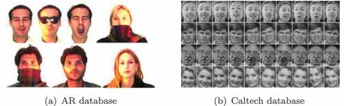
In this experiment, we use two standard and challenging face recognition databases. The first database is the AR face database, which has 4000 color images corresponding to 126 people’s faces (70 men and 56 women). Images feature frontal view faces with different facial expressions, illumination conditions, and occlusions (sunglasses and scarf). The second database is Caltech faces by California Institute of Technology, consists of 450 face images of around 27 unique people (both genders) with different lighting/expressions/backgrounds (sample images are shown in Figure 1. We apply bag of feature (BOF) for representing the image vectors where SIFT has been used for feature extraction, treating the local image patches as the visual equivalent of individual words.

Figure 1. Sample from face recognition database.

Figures 2 and 3 show that our proposed approaches permit good discrimination. The intraclass performance for the AR using proposed approaches is shown in Figure 3. We note that InfEMSSD-MCMC shows superior performance in distinguishing women class ($97\mathrm{\%}$) from men class ($94\mathrm{\%}$) and InfEMBL-MCMC achieves $96.01\mathrm{\%}$ in Caltech data set as we can see in Figure 2. Overall, all of our proposed models and algorithms ensure an accuracy above 85 $\mathrm{\%}$ in this application. Compared with the EM algorithm, our proposed MCMC algorithms show higher accuracy with the corresponding models.

Figure 2. Intraclass accuracy for proposed approaches models in Caltech data.

Figure 3. Intraclass accuracy for proposed approaches models in AR data.

Conclusion

In this paper, we have proposed a novel approach for finite mixtures of EMGD, EMBL and EMSSD based on the development of conjugate prior distributions and on the Monte Carlo simulation techniques of Gibbs sampling mixed with a M–H step. Generally, with the help of prior information and the stochastic aspect of the simulation in Gibbs sampling, our proposed algorithms ensure accurate models learning. Moreover, via a Bayesian nonparametric extension based on these mixtures, we show that the problem of determining the number of clusters can be cured and avoided by using infinite mixtures which model well the structure of the data. Our proposed approaches and infinite models offer excellent modeling capabilities as shown in the experimental part, which involves text sentiment analysis, fake news detection and human face recognition, compared to the widely used maximal likelihood approaches in high-dimensional count data. However, our modeling framework still has some drawbacks as follows. First, the high computational complexity of the proposed inference led to slow convergence. A promising future work could be replacing the classical M–H by the Scalable M–H algorithm proposed in Cornish et al. (2019). This scheme is based on combination of factorized acceptance probabilities, procedures of Bernoulli processes, and control variate idea. It can be used to reduce the computational complexity by discovering in advance the sampling points that may be rejected. Second, Gibbs sampling might take a long time to converge. When two or more mixture components have similar parameters, the Gibbs sampling method can get stuck in a local mode, resulting in inaccurate data points clustering. A possible solution that could be investigated is to consider the spilt-merge Markov Chain Monte Carlo procedure for the Dirichlet process as described in Jain and Neal (2004). Finally, the proposed approaches may be sensitive to the choice of the hyperparameters values. A potential future work could be devoted to developing an approach for the automatic selection of these values depending on the data to model.

Acknowledgments

The authors would like the thank the associate editor and the reviewers for their comments and suggestions that helped to improve the paper.

Disclosure Statement

No potential conflict of interest was reported by the author(s).

Additional information

Funding

This work was supported by the Natural Sciences and Engineering Research Council of Canada [6656-2017].

Appendix A

Proof of Equation 17(17) $\begin{array}{cc}p(\mathbf{Z}|\eta )& =\int P(\mathbf{Z}|P_{inf})P(P_{inf}|\eta )\\ \hspace{0.17em}& =\frac{\mathrm{\Gamma }(\eta )}{\mathrm{\Gamma }{(\eta /M)}^M}\int \prod _{j=1}^M{\pi }^{n_j+\eta /M-1}d{\pi }_j\\ \hspace{0.17em}& =\frac{\mathrm{\Gamma }(\eta )}{\mathrm{\Gamma }(N+\eta )}\prod _{j=1}^M\frac{\mathrm{\Gamma }(n_j+\eta /M)}{\mathrm{\Gamma }(\eta /M)}\end{array}$(17)

(A1) $\begin{array}{cc}\pi ({\xi }_j|\mathbf{M},\mathbf{X})& \propto \pi ({\xi }_j)\prod _{Z_{ij}=1}EGDM(X_i|{\xi }_j)\\ \hspace{0.17em}& =exp(\sum _{w=1}^W{\rho }_{l}log\frac{{\alpha }_w{\beta }_w}{{\alpha }_w+{\beta }_w})\prod _{Z_{ij}=1}\{(\prod _{W:x_W\ge 1}{x}_w^{-1})\prod _{W:x_W\ge 1}\frac{\mathrm{\Gamma }(z_w)}{\mathrm{\Gamma }(x_w+z_w)}n\\ \hspace{0.17em}& \times \{exp\sum _{w=1}^{W}I(x_w>=1)log\frac{{\alpha }_w{\beta }_w}{{\alpha }_w+{\beta }_w}\}\}\end{array}$(A1)

Removing the equation parts which is only related with data set $\mathcal{X}$, because it does not have an effect on the r calculation in M–H step.

(A2) $\begin{array}{cc}\pi ({\xi }_j|\mathbf{M},\mathbf{X})& \propto \pi ({\mathrm{\Theta }}_j)\prod _{Z_{ij}=1}EGDM(X_i|{\mathrm{\Theta }}_j)\\ \hspace{0.17em}& \propto exp[\sum _{w=1}^{W}log\frac{{\alpha }_w{\beta }_w}{{\alpha }_w+{\beta }_w}({\rho }_w+\sum _{Z_{ij}=1}^{N}I(x_{iw}\ge 1))]\\ \hspace{0.17em}& \times \prod _{Z_{ij}=1}^N(\prod _{w:x_{iw}\ge 1}{x}_{iw}^{-1}\frac{\mathrm{\Gamma }(z_{iw})}{\mathrm{\Gamma }(x_{iw}+z_{iw})}n!)\end{array}$(A2)

Appendix B

Proof of Equation 21(21) $p(\eta |\vartheta ,\rho ,M,N)=\frac{{\rho }^{\vartheta }exp(-\rho /\eta )}{\mathrm{\Gamma }(\vartheta ){\eta }^{\vartheta +1}}\times \frac{{\eta }^M\mathrm{\Gamma }(\eta )}{\mathrm{\Gamma }(N+\eta )}$(21)

(B1) $\begin{array}{cc}\pi ({\xi }_j|\mathbf{M},\mathbf{X})& \propto \pi ({\xi }_j)\prod _{Z_{ij}=1}EMBL(X_i|{\xi }_j)\\ \hspace{0.17em}& =exp[\sum _{w=1}^W{\rho }_{d}log({\alpha }_d)+k(log(\frac{\mathrm{\Gamma }(S)\mathrm{\Gamma }({\alpha }^{\mathrm{\prime }})\mathrm{\Gamma }({\beta }^{\mathrm{\prime }})\alpha }{\mathrm{\Gamma }(S+n)\mathrm{\Gamma }({\alpha }^{\mathrm{\prime }}+{\beta }^{\mathrm{\prime }})}))]\\ \hspace{0.17em}& \times \prod _{Z_{ij}=1}\{(\prod _{d:x_d>=1}{x}_d^{-1})n!\frac{\mathrm{\Gamma }(S)\mathrm{\Gamma }({\alpha }^{\mathrm{\prime }})\mathrm{\Gamma }({\beta }^{\mathrm{\prime }})\alpha }{\mathrm{\Gamma }(S+n)\mathrm{\Gamma }({\alpha }^{\mathrm{\prime }}+{\beta }^{\prime })}\times exp\{\sum _{d=1}^{D}I(x_d\le 1)log({\alpha }_d)\}\}\\ \hspace{0.17em}& =\prod _{Z_{ij}=1}(\prod _{d:x_d>=1}{x}_d^{-1}n!)exp[\sum _{w=1}^{W}log({\alpha }_w)({\rho }_w+\sum _{Z_{ij}=1}^{N}I(x_{iw}\ge 1))\\ \hspace{0.17em}& +k(log(\frac{\mathrm{\Gamma }(S)\mathrm{\Gamma }({\alpha }_j^{\mathrm{\prime }})\mathrm{\Gamma }({\beta }_j^{\mathrm{\prime }}){\alpha }_j}{\mathrm{\Gamma }(S+n)\mathrm{\Gamma }({\alpha }_j^{\mathrm{\prime }}+{\beta }_j^{\mathrm{\prime }})}))\\ \hspace{0.17em}& \hspace{0.17em}\end{array}$(B1)

We remove the equations which are only related with data set $\mathcal{X}$.

For the fact that:

(B2) $\mathrm{\Gamma }(S+n)=\mathrm{\Gamma }(S)(S)\times (S+1)\cdots (S+n-1)$(B2)

So we have this:

(B3) $\propto exp[\sum _{w=1}^{W}log({\alpha }_w)({\rho }_w+\sum _{Z_{ij}=1}^{N}I(x_{iw}\ge 1))+k(log(\frac{\mathrm{\Gamma }({\alpha }_j^{\mathrm{\prime }})\mathrm{\Gamma }({\beta }_j^{\mathrm{\prime }}){\alpha }_j}{(S)\times (S+1)\cdots (S+n-1)\mathrm{\Gamma }({\alpha }_j^{\mathrm{\prime }}+{\beta }_j^{\mathrm{\prime }})}))+\sum _{i=1,z_{ij}=1}(log(\frac{\mathrm{\Gamma }({\alpha }^{\mathrm{\prime }})\mathrm{\Gamma }({\beta }^{\mathrm{\prime }})\alpha }{(S)\times (S+1)\cdots (S+n-1)\mathrm{\Gamma }({\alpha }^{\mathrm{\prime }}+{\beta }^{\mathrm{\prime }})}))]$(B3)

Appendix C.

Conditional Posterior of model hyperparmeters

In EMGD, those conditional posteriors becomes:

(C1) $\begin{array}{cc}p(|\cdots )& \propto p()\prod _{j=1}^{M}p({\alpha }_j|\delta ,)\\ \hspace{0.17em}& \lambda exp(-\lambda )\\ \hspace{0.17em}& \prod _{j=1}^M\times \frac{\mathrm{\Gamma }(\delta +)}{\mathrm{\Gamma }(\delta )\mathrm{\Gamma }()}{\alpha }_j^{\delta -1}{(1-{\alpha }_j)}^{-1}\end{array}$(C1)

(C2) $\begin{array}{cc}p(\delta |\cdots )& \propto p(\delta )\prod _{j=1}^{M}p({\alpha }_j|\delta ,)\\ \hspace{0.17em}& \frac{\mathrm{\Gamma }(\varsigma +\upsilon )}{\mathrm{\Gamma }(\varsigma )\mathrm{\Gamma }(\upsilon )}{\delta }^{\varsigma -1}{(1-\varsigma )}^{\upsilon -1}\\ \hspace{0.17em}& \times \frac{\mathrm{\Gamma }(\delta +)}{\mathrm{\Gamma }(\delta )\mathrm{\Gamma }()}{\alpha }_j^{\delta -1}{(1-{\alpha }_j)}^{-1}\end{array}$(C2)

(C3) $\begin{array}{cc}p(\rho |\cdots )& \propto p(\rho )\prod _{j=1}^{M}p({\beta }_j|\varpi ,\rho )\\ \hspace{0.17em}& =\iota exp(-\iota \rho )\\ \hspace{0.17em}& \times \prod _{j=1}^M\frac{\mathrm{\Gamma }(\varpi +\rho )}{\mathrm{\Gamma }(\varpi )\mathrm{\Gamma }(\rho )}{\beta }_j^{\varpi -1}{(1-{\beta }_j)}^{\rho -1}\end{array}$(C3)

(C4) $\begin{array}{c}p(\varpi |\cdots )\propto p(\varpi ))\prod _{j=1}^{M}p({\beta }_j|\varpi ,\rho )\\ =\frac{\mathrm{\Gamma }(\kappa +\omega )}{\mathrm{\Gamma }(\kappa )\mathrm{\Gamma }(\omega {\varpi }^{\kappa -1}{(1-\kappa )}^{\omega -1}}\\ \hspace{0.17em}\times \prod _{j=1}^M\frac{\mathrm{\Gamma }(\varpi +\rho )}{\mathrm{\Gamma }(\varpi )\mathrm{\Gamma }(\rho )}{\beta }_j^{\varpi -1}{(1-{\beta }_j)}^{\rho -1}\end{array}$(C4)

In EMBL, the form of $p(|\cdots )$ and $p(\delta |\cdots )$ are same in Equation (C1) and Equation (C2). the conditional posterior for $\rho$ and $\varpi$, we have:

(C5) $\begin{array}{cc}p(\rho |\cdots )& \propto p(\rho )\prod _{j=1}^{M}p({\beta }_j|\varpi ,\rho )\\ \hspace{0.17em}& =\iota exp(-\iota \rho )\prod _{j=1}^M\frac{{\rho }^{\varpi }exp(-\rho /{\beta }_j)}{\mathrm{\Gamma }(\varpi ){\beta }_j^{\varpi -1}}\end{array}$(C5)

(C6) $\begin{array}{cc}p(\varpi |\cdots )& \propto p(\varpi )\prod _{j=1}^{M}p({\beta }_j|\varpi ,\rho )\\ \hspace{0.17em}& =\frac{{\omega }^{\kappa }exp(-\omega /\varpi )}{\mathrm{\Gamma }(\kappa ){\varpi }^{\kappa -1}}\prod _{j=1}^M\frac{{\rho }^{\varpi }exp(-\rho /{\beta }_j)}{\mathrm{\Gamma }(\varpi ){\beta }_j^{\varpi -1}}\end{array}$(C6)

References

- Alsuroji, R., N. Zamzami, and N. Bouguila. 2018. “Model selection and estimation of a finite shifted-scaled dirichlet mixture model.” In 17th IEEE International Conference on Machine Learning and Applications, ICMLA 2018, Orlando, FL, USA, December 17-20, edited by M. A. Wani, M. M. Kantardzic, M. S. Mouchaweh, J. Gama, and E. Lughofer, 707–2542. IEEE.
- Amirkhani, M., N. Manouchehri, and N. Bouguila. 2021. Birth-death MCMC approach for multivariate beta mixture models in medical applications. In Advances and trends in artificial intelligence. artificial intelligence practices, ed. H. Fujita, A. Selamat, J. C.-W. Lin, and M. Ali, 285–96. Cham: Springer International Publishing.
- Antoniak, C. E. 1974. Mixtures of dirichlet processes with applications to bayesian nonparametric problems. The Annals of Statistics 2 (6):1152–74. doi:10.1214/aos/1176342871.
- Batista, L., and S. Ratté. 2014. Multi-classifier system for sentiment analysis and opinion mining. In Encyclopedia of social network analysis and mining, ed. R. Alhajj and J. Rokne, 989–98. New York: Springer New York.
- Bouguila, N. 2008. Clustering of count data using generalized dirichlet multinomial distributions. IEEE Transactions on Knowledge and Data Engineering 20 (4):462–74. doi:10.1109/TKDE.2007.190726.
- Bouguila, N. 2011. Count data modeling and classification using finite mixtures of distributions. IEEE Transactions on Neural Networks 22 (2):186–98. doi:10.1109/TNN.2010.2091428.
- Bouguila, N., and W. Fan. 2020. Mixture models and applications. Springer.
- Bouguila, N., and D. Ziou. 2007. Unsupervised learning of a finite discrete mixture: Applications to texture modeling and image databases summarization. Journal of Visual Communication and Image Representation 18 (4):295–309. doi:10.1016/j.jvcir.2007.02.005.
- Bouguila, N., and D. Ziou. 2010. A Dirichlet process mixture of generalized Dirichlet distributions for proportional data modeling. IEEE Transactions on Neural Networks 21 (1):107–22. doi:10.1109/TNN.2009.2034851.
- Bouguila, N., D. Ziou, and R. I. Hammoud. 2009. On Bayesian analysis of a finite generalized dirichlet mixture via a Metropolis-within-Gibbs sampling. Pattern Analysis and Applications 12 (2):151–66. doi:10.1007/s10044-008-0111-4.
- Brooks, S. P. 2001. On Bayesian analyses and finite mixtures for proportions. Statistics and Computing 11 (2):179–90. doi:10.1023/A:1008983500916.
- Brown, L. D. 1986. Fundamentals of statistical exponential families with applications in statistical decision theory. Lecture Notes-Monograph Series 9:100–279.
- Cai, L. 2010. High-dimensional exploratory item factor analysis by a Metropolis–Hastings Robbins–Monro algorithm. Psychometrika 75 (1):33–57. doi:10.1007/s11336-009-9136-x.
- Church, K. W., and W. A. Gale. 1995. Poisson mixtures. Natural Language Engineering 1 (2):163–90. doi:10.1017/S1351324900000139.
- Cornish, R., P. Vanetti, A. Bouchard-Cote, G. Deligiannidis, and A. Doucet. 2019. “Scalable Metropolis–Hastings for exact Bayesian inference with large datasets.” In International Conference on Machine Learning, 1351–60.
- DasGupta, A. 2011. The exponential family and statistical applications. In Probability for statistics and machine learning. edited by Anirban DasGupta, 583–612. New York, NY: Springer.
- Dhillon, I. S., and D. S. Modha. 2001. Concept decompositions for large sparse text data using clustering. Machine Learning 42 (1/2):143–75. doi:10.1023/A:1007612920971.
- Dias, J. G., and M. Wedel. 2004. An empirical comparison of EM, SEM and MCMC performance for problematic gaussian mixture likelihoods. Statistics and Computing 14 (4):323–32. doi:10.1023/B:STCO.0000039481.32211.5a.
- Elkan, C. 2006. “Clustering documents with an exponential-family approximation of the dirichlet compound multinomial distribution.” In Proceedings of the 23rd International Conference on Machine Learning, ICML ‘06, New York, NY, USA, 289–96. Association for Computing Machinery.
- Emanuel, L., and G. T. Herman. 1987. A maximum a posteriori probability expectation maximization algorithm for image reconstruction in emission tomography. IEEE Transactions on Medical Imaging 6 (3):185–92. doi:10.1109/TMI.1987.4307826.
- Escobar, M. D., and M. West. 1995. Bayesian density estimation and inference using mixtures. Journal of the American Statistical Association 90 (430):577–88. doi:10.1080/01621459.1995.10476550.
- Favaro, S., and Y. Whye Teh. 2013. MCMC for normalized random measure mixture models. Statistical Science 28 (3):335–59. doi:10.1214/13-STS422.
- Hartigan, J., and M. Wong. 1979. Algorithm AS 136: A K-Means Clustering Algorithm. Journal of the Royal Statistical Society 28 (1):100–08.
- Jain, A. K. 2010. Data clustering: 50 years beyond K-means. Pattern Recognition Letters 31 (8):651–66. doi:10.1016/j.patrec.2009.09.011.
- Jain, S., and R. Neal. 2004. A split-merge markov chain monte carlo procedure for the dirichlet process mixture model. Journal of Computational and Graphical Statistics 13 (1):158–82. doi:10.1198/1061860043001.
- Jegou, H., M. Douze, and C. Schmid. 2009. On the burstiness of visual elements. In 2009 IEEE Conference on Computer Vision and Pattern Recognition, 1169–76.
- Katz, S. M. 1996. Distribution of content words and phrases in text and language modelling. Natural Language Engineering 2 (1):15–59. doi:10.1017/S1351324996001246.
- Korwar, R. M., and M. Hollander. 1973. Contributions to the theory of dirichlet processes. The Annals of Probability 1 (4):705–11. doi:10.1214/aop/1176996898.
- Lee, P. M. 2012. Bayesian Statistics: An Introduction. Wiley.
- MacEachern, S. N., and P. Muller. 1998. Estimating mixture of dirichlet process models. Journal of Computational and Graphical Statistics 7:223–38.
- Madsen, R. E., D. Kauchak, and C. Elkan. 2005. “Modeling WORD BURSTINESS USING THE DIRICHLET DISTRIBUTION.” In Proceedings of the 22nd International Conference on Machine Learning, ICML ‘05, New York, NY, USA, 545?552. Association for Computing Machinery.
- Margaritis, D., and S. Thrun. 2001. A bayesian multiresolution independence test for continuous variables. In Proceedings of the Seventeenth Conference on Uncertainty in Artificial Intelligence, 346–53. Morgan Kaufmann Publishers Inc.
- Najar, F., N. Zamzami, and N. Bouguila. 2019. “Fake news detection using bayesian inference.” In 2019 IEEE 20th International Conference on Information Reuse and Integration for Data Science (IRI), 389–94.
- Najar, F., N. Zamzami, and N. Bouguila. 2020. “Recognition of human interactions in feature films based on infinite mixture of EDCM.” In 2020 International Symposium on Networks, Computers and Communications (ISNCC), 1–6.
- Raftery, A. E., and S. M. Lewis. 1992. [Practical markov chain monte carlo]: comment: one long run with diagnostics: implementation strategies for markov chain monte Carlo. Statistical Science 7 (4):493–97. doi:10.1214/ss/1177011143.
- Rasmussen, C. E. 1999. The infinite Gaussian mixture model. Advances in Neural Information Processing Systems 12:554–60.
- Robert, C. P. 2007. The Bayesian choice. From decision-theoretic foundations to computational implementation. Springer.
- Roeder, K., and L. Wasserman. 1997. Practical bayesian density estimation using mixture of normals. Journal of the American Statistical Association 92 (439):894–902. doi:10.1080/01621459.1997.10474044.
- Samuel, K., N. Balakrishnan, and N. L. Johnson. 2000. Continuous multivariate distributions. New York: Wiley-Interscience.
- Sorensen, D., and D. Gianola. 2002. Likelihood, Bayesian and MCMC methods in quantitative genetics. Springer.
- Train, K. E. 2009. Discrete choice methods with simulation. 2nd ed. Cambridge University Press.
- Tsionas, E. G. 2004. Bayesian inference for multivariate gamma distributions. Statistics and Computing 14 (3):223–33. doi:10.1023/B:STCO.0000035302.87186.be.
- Wong, T.-T. 2010. Parameter estimation for generalized Dirichlet distributions from the sample estimates of the first and the second moments of random variables. Computational Statistics & Data Analysis 54 (7):1756–65. doi:10.1016/j.csda.2010.02.008.
- Xuanbo, S., N. Bouguila, and N. Zamzami. 2021. “Covid-19 News Clustering using MCMC-Based Learing of finite EMSD Mixture Models.” In Proceedings of the Thirty-Fourth International Florida Artificial Intelligence Research Society Conference, North Miami Beach, Florida, USA, May 17-19, edited by E. Bell and F. Keshtkar.
- Zamzami, N., and N. Bouguila. 2019. A novel scaled Dirichlet-based statistical framework for count data modeling: Unsupervised learning and exponential approximation. Pattern Recognition 95:36–47. doi:10.1016/j.patcog.2019.05.038.
- Zamzami, N., and N. Bouguila. 2020a. High-dimensional count data clustering based on an exponential approximation to the multinomial Beta-Liouville distribution. Information Sciences 524:116–35. doi:10.1016/j.ins.2020.03.028.
- Zamzami, N., and N. Bouguila. 2020b. Probabilistic modeling for frequency vectors using a flexible shifted-scaled dirichlet distribution prior. ACM Trans. Knowl. Discov. Data 14 (6):1–35. doi:10.1145/3406242.
- Zamzami, N., and N. Bouguila. 2022. Sparse count data clustering using an exponential approximation to generalized dirichlet multinomial distributions. IEEE Transactions on Neural Networks and Learning Systems 33 (1):89–102. doi:10.1109/TNNLS.2020.3027539.
Appendix A
Proof of EquationEquation 17 (17) (17)