Pattern-of-Life Activity Recognition In Seismic Data

ABSTRACT

Pattern-of-life analysis models the observable activities associated with a particular entity or location over time. Automatically finding and separating these activities from noise and other background activity presents a technical challenge for a variety of data types and sources. This paper investigates a framework for finding and separating a variety of vehicle activities recorded using seismic sensors situated around a construction site. Our approach breaks the seismic waveform into segments, preprocesses them, and extracts features from each. We then apply feature scaling and dimensionality reduction algorithms before clustering and visualizing the data. Results suggest that the approach effectively separates the use of certain vehicle types and reveals interesting distributions in the data. Our reliance on unsupervised machine learning algorithms suggests that the approach can generalize to other data sources and monitoring contexts. We conclude by discussing limitations and future work.

Introduction

Pattern-of-life (PoL) analysis refers to the surveillance of an entity or location to learn about common or repeating activities happening over a period of time (Craddock, Watson, and Saunders 2016). As a very simple example, consider traffic counters, which can count, classify, and measure the speed of vehicles along a given stretch of road. Such data is used to determine traffic light timing, local speed limits, placement of road improvement projects, and even police enforcement efforts. The resulting data stream can also be mined for more complex temporal patterns, such as rush-hour timing, weekend and holiday effects, or changes induced in heavy vehicle usage by opening or closing of local businesses. Variants of pattern-of-life analysis arise in financial data, such as credit card fraud detection, and social media platforms, such as targeting advertisements or news articles.

The entity surveyed in our study is a construction site outfitted with seismic sensors around its perimeter. Relevant activities at the site include operation of vehicles, such as cranes, forklifts or dump trucks, throughout a given day. The analytic task is to automatically separate and model these activities. Although beyond the scope of this paper, the resulting activity models can be used to predict future actions or detect anomalies. For example, a dump truck bringing gravel to the construction site is a strong indicator that a frontend loader or bulldozer will soon follow to disperse the gravel. An anomaly might include an accident, such as a crane load becoming loose and falling to the ground.

Using seismic sensors for surveillance has its own set of unique challenges and advantages due to the nature of seismic waves. Seismic sensors can detect any energy that reaches the sensor, including irrelevant natural seismic activity and anthropogenic activity from elsewhere. Seismic waves are also highly influenced by the underlying geology, so making prior assumptions about wave shapes and propagation can lead to misinterpretation. For these reasons, separating the seismic signal of an activity from noise is a challenging process that requires in-depth analysis of the seismic data. In spite of these challenges, the incorporation of seismic sensors in PoL analysis serves as a promising source of data when the line of sight cannot be established or when temporal resolution is important.

Our contributions can be summarized as follows: (1) We develop an unsupervised machine learning framework for discovering anthropogenic activities captured with a single seismic sensor. (2) We identify the necessary steps for this type of data and analysis, including preprocessing, data segmentation, dimensionality reduction, and clustering. (3) We use traditional and statistical clustering evaluation metrics on a set of experiments to determine how well our framework can separate different classes of activities. (4) We provide an in-depth discussion about the limitations of our framework, properties of the dataset, possible directions for future research, and implications for PoL analysis.

Background and Related Work

Most existing research on seismic analysis of anthropogenic activity uses supervised machine learning methods for a wide range of applications. Much of this work focuses on extracting a set of features from seismic data from one or more of the following domains: time, frequency, or time–frequency. Time domain methods extract features from the seismogram (raw signal) itself. Frequency domain methods extract features from representations of the signal that contain information about frequency content, such as a Fourier transform. Time–frequency domain methods extract features from representations of the signal that reveal frequency content and the time associated with those frequencies, like the wavelet transformation. Most research in seismic data analysis focuses on extracting features from the time–frequency and frequency domains.

Many previous works use supervised or semi-supervised machine learning models to classify seismic data. Ghosh and Sardana (2020, June) classifies seismic and acoustic time series using features extracted from the time, frequency, and time–frequency domains. Kalra, Kumar, and Das (2020) uses empirical wavelet transformation to find features in the time–frequency domain to classify seismic segments such as bus, tractor, or noise. Conversely, Kalra, Kumar, and Das (2018) extracts time–frequency coefficients by using the smooth-pseudo Wigner-Ville distribution technique to detect the presence of a target. Ntalampiras (2018) extracts features from the frequency domain and analyzes dependency among acoustic sequences before classifying. Ghosh et al. (2015) determined vehicle presence based on energy distribution in the time–frequency domain. Huang et al. (2013) found time–frequency domain features using an algorithm called wavelet packet manifold. Jin et al. (2011) created a symbolic representation of wavelet transformations to classify seismic activity from humans, animals, and vehicles. William and Hoffman (2011) classified different military ground vehicles based on time–frequency domain harmonics.

These methods assume seismic activity generated by ground targets of interest are isolated, and therefore the start and end times of an activity in the waveform are easily located. In this relatively simple scenario, features from the time–frequency domain, which have information about the frequency content and where the frequencies appear in the signal, are very useful for finding signatures in the seismic data. However, for a more realistic PoL analysis scenario, determining when specific activities begin and end is very challenging. In practice, supervised approaches that rely on a training set are unrealistic. Different vehicles (make and model) or equipment (bulldozer versus loader) may be used to perform a given task at a construction site. For example, if there are small and large cranes onsite, the large crane may be used to perform tasks typically assigned to the small crane, thereby changing the signature of the activity in the seismic data. Unsupervised methods may therefore be more appropriate.

Unsupervised machine learning methods for seismic analysis of anthropogenic activities exist in the literature, but ours is the first to apply an unsupervised framework to a wide range of activities from a single sensor. Recently, Snover et al. (2021) used deep neural networks to cluster seismic sequences in order to distinguish novel seismic signals from noise. Johnson et al. (2020) used unsupervised learning to identify different levels of seismic noise. Chamarczuk et al. (2020) used clustering to detect and categorize seismic events. Riahi and Gerstoft (2017) focused on using graph clustering to separate seismic activity generated from helicopters and oil processing plants. However, these works applied their methods to a large and dense array of seismic sensors and leveraged the spatiotemporal information inherent in the array to help categorize seismic data. Our PoL scenario focuses on one seismic sensor only.

Importantly, PoL analysis often assumes little about the set of activities present in the data. Taking an unsupervised approach can also be difficult due to the number and variety of activities, changing levels of noise throughout the day, and variance in the signatures for functionally equivalent activities. Importantly, these sources of variance can impact what gets detected and what does not when tuning hyper-parameters of an unsupervised segmentation method. Thus, segmenting individual activities from the waveform by identifying start and end times in active PoL scenarios, such as our construction site, is imprecise at best. Alternatively, a sub-sequencing approach, where a sliding window of fixed size and overlap with the previous window, could be taken. However, sub-sequencing makes time–frequency domain feature extraction methods much less effective at distinguishing different activities because information about where the frequencies are present in the seismic signal no longer matter as frequencies may be broken across multiple windows.

Due to the success of methods based on time–frequency domain feature in ground target identification problems, few methods based on frequency domain features extraction exist. However, Tian, Qi, and Wang (2002) created an algorithm called Spectral Statistics and Wavelet Coefficients Characterization (SSWCC), to extract features from both the frequency and time–frequency domains. The algorithm extracts features by calculating shape statistics of the Fourier transformation, power spectral density, and wavelet transformation of the seismic signal. SSWCC helps us negate the loss in effectiveness of using features from the time–frequency domain, caused by our sub-sequencing approach, by incorporating features from the frequency domain. Because of this benefit, we use SSWCC as our feature extraction method in our pattern of life activity recognition framework. This algorithm is explained further in a later section.

Activity Categorization Framework

An overarching goal of pattern-of-life analysis is to predict future actions at a given site under surveillance. This is equally true of pattern analysis in financial or social domains as in sensor domains. To establish activity patterns and make predictions, we first need to recognize and distinguish among individual activities. In this section, we describe our seismic data and the framework developed for separating different types of anthropogenic activity captured by the sensors.

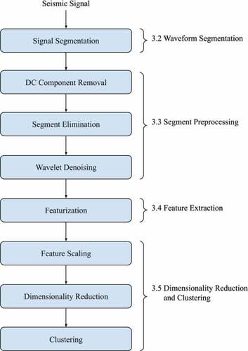
Figure 1 shows a flowchart for our framework. The method begins by breaking the seismic time series into short overlapping time segments. Next, each segment is preprocessed to remove the Direct Current (DC) component, which reduces noise and ensures that the power can be calculated accurately. Next, segments with insufficient power are eliminated as they are unlikely to be capturing any activity. Preprocessing concludes with wavelet denoising and high-pass filtering, which reduces noise from natural seismic activity and off-site anthropogenic activity. Next, we extract features from each segment and apply scaling and dimensionality reduction. Lastly, we cluster on the scaled and reduced features of each segment in an effort to separate different types of vehicles – without providing hints on the classes of activity present. We validate our results using labeled data to highlight the characteristics of different cluster distributions from several classes that represent operation of specific vehicles. The following sections provide details on each analysis stage.

Figure 1. Flowchart describing the stages of unsupervised on-site activity detection for seismic data.

The Dataset

Our dataset consists of daily seismic recordings over a period of several months. The full dataset is used in our analysis to determine which frequencies relate to noise and to determine which segments capture activity from the construction site. We test our framework on a subset of six sequential days of seismic recordings selected for their variety of recorded activity. These recordings came from a single INOVA Hawk geophone recording at 500 Hz, located approximately 500 m from the target construction site. The geophone is equipped with three analog channels and three digital channels. The analog data were digitized using a 24-bit Delta-Sigma covertor. Anti-aliasing was applied at 206 Hz.

The dataset also contains construction logs for each day. The construction logs provide information about which vehicles were operated on a certain day, but they do not specify when they were operated. The construction logs allow us to establish 24-hour periods of seismic recordings with no onsite activity and 24-hour periods with heavy onsite activity. These 24-hour periods are used to help guide our decisions for preprocessing the segments. This process is fully explained in Section 3.3.

For the purposes of this study, activities of the construction site are defined as the operation of specific vehicles at the site. The construction site includes the operation of many different types of vehicles. The semi-trailer and semi-flatbed are large diesel powered trucks used to haul large objects. The cranes are of different sizes, diesel powered, and tracked. The heavy pickup truck, septic truck, boxy tank truck, and water truck are all smaller than the semi-trucks, diesel powered, and wheeled vehicles. The forklift and frontend loader are diesel-powered construction equipment, larger than the trucks with larger wheels. The covering for rain activity captures seismic activity from the movement of workers as they put up covering to protect equipment from rain.

A time-lapse video camera (10 seconds per frame) with a partial field of view of the construction site and no audio captures vehicle operation occurring onsite. The video data helped to establish ground truth of when activities began and ended. Ground truth labels of activities can only be established when vehicles are moving. Vehicles in operation but remaining stationary, or vehicles outside the field of view of the camera, may generate seismic signals but are not labeled, as we cannot determine whether the engines are running and generating signals. Rarely, more than one vehicle could be seen operating, no label was associated for these time periods.

In a real-world deployment for PoL analysis, if several vehicles operate together, they will either form their own cluster or the vehicle generating the most seismic activity will cause the segment to cluster with segments only associated with said vehicle. If the operation of the several vehicles together is infrequent, the associated cluster may be considered noise and ignored in further PoL analysis. If it frequently occurs, then it may be treated as its own activity like the operation of only one vehicle. In practice, there may be several ways to handle simultaneous activities, depending on the specifics of the data. We have not explored the space in detail.

Waveform Segmentation

Research on seismic activity from vehicles shows that the waves travel as Rayleigh waves (Lan et al. 2005). Rayleigh waves are surface waves that travel in both the direction of propagation and perpendicular to it (in the vertical plane). Based on this research and to simplify our analysis, we only use the vertical direction of our three-axial seismic sensor.

The seismic recording for the selected 6 days is sub-sequenced into overlapping segments. In total, there are 14,000 segments, 10 seconds in length, in our dataset. Segments are labeled according to the established ground truth from the video data. We use the labeled segments to validate the final cluster results by checking if similar activities cluster together. Table 1 shows the different classes of activities and the frequency of their occurrence in the segments. Most were not associated with any label. However, a segment without a label may still correspond to an activity, such as a vehicle in operation but running idle on the construction site.

Table 1. Frequency of activities.

Activity	Frequency
No Label	11415
Heavy Pickup	29
Semi-Trailer	708
Frontend Loader	872
Forklift	15
Water Truck	527
Medium Crane	91
Large Tank Truck	125
Septic Truck	111
Covering For Rain	19
Large Crane	226
Semi-Flatbed	62

Initially, we tried several methods for automatic seismic event detection and segmentation. These methods include Short-Term Average over Long-Term Average (STA/LTA) (Allen 1982), which is a traditional seismic event detection technique, along with time-series segmentation methods like Pelt (Killick, Fearnhead, and Eckley 2012), binary segmentation (Scott and Knott 1974), bottom-up segmentation, window-based segmentation, and Bayesian techniques (Adams and MacKay 2007). However, all methods performed poorly, often failing to detect some activities or detecting many change points when none were present. Slight adjustments of hyper-parameters produced very different results, indicating that these methods were very sensitive to the details of the data. The failure of traditional detection methods on the construction site data was expected, as the signals generated by heavy equipment are different from the earthquakes and mining explosions for which these methods are typically used.

Seismic signals emanating from the construction site are complex and varied, introducing both slow gradual changes and abrupt changes to the seismic time series. We therefore segmented the data using a sliding window with 10% overlap in lieu of traditional segmentation methods. The length of the segments is set to 10 seconds and chosen based on pilot clustering experiments. Shorter segments, especially those shorter than 7 seconds, tended to fall into a single cluster. Longer segments of 12 seconds or more produced separate clusters, but these clusters were less homogeneous in terms of labels. The overlap percentage was also chosen based on pilot clustering experiments. Decreasing the overlap percentage resulted in fewer, sparse, and less homogeneous clusters. Increasing the overlap percentage resulted in several small, dense, and more homogeneous clusters, up to a certain percentage, afterward clusters merge and become less homogeneous.

Segment length and overlap percentage are two important hyper-parameters that greatly influence the resulting clusters. In theory, the segment length controls the level of granularity that can be captured from on-site activities. Initial experiments showed that a segment length of 5–7 seconds can capture different types of movement coming from one vehicle. For example, with a segment length of 5–7 seconds, we were able to separate arm movement, pivoting in place, and moving forward for a large crane. Using a longer segment length of 10–15 seconds tended to merge these movements into a single general group for large crane operation. Even longer segment lengths (30 seconds or more) may be better suited for capturing overall processes such as digging a hole. The overlap percentage controls intercluster and intracluster distances. Segments from the same activity with high percentages of overlap share more data and therefore have low intercluster distance (high density). However, intracluster distances may decrease too much with a high percentage of overlap, causing merging between clusters/separate activities. In practice, the overlap percentage should be set as high as possible before clusters start to merge. This analysis can easily be done with basic methods such as silhouette score.

Segment Preprocessing

We use Probabilistic Power Spectral Density (PPSD) (McNamara and Boaz 2006) to help with preprocessing decisions. PPSD allows us to plot possible frequencies in the seismic data with high amounts of energy related to on-site activity. Figure 2 shows a PPSD plot of a day with no site activity and a PPSD plot of a day with heavy site activity. Frequency (Hz) is on the x-axis and power/amplitude (dB) is on the y-axis. The colors in the bins indicate the percentage of 30-second segment spectra passing through the frequency/amplitude bin as shown by the color bar. The gray lines are the Peterson high- and low-noise models plotted for reference (Vasco, Peterson, and Majer 1996). Ninety-five percent of the 30-second segment spectra are contained between the black lines. The 40 Hz frequency is marked by the yellow line. The red line on the right plot reflects the upper 95th percentile line from the left plot.

Figure 2. Probabilistic power spectral density plots for site activity. Each plot is divided into bins based on frequency and amplitude, represented by the grid. The color bar on the right indicates the percentage of segment spectra passing through a specific bin. 95% of segment spectra are contained between the black lines. The red line of the site activity plot references the upper 95th percentile line of the no site activity plot. The vertical yellow line marks the frequency of 40 Hertz.

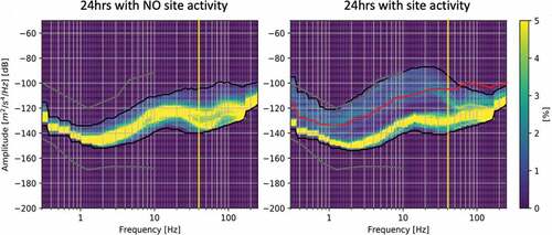
The PPSD plots in Figure 2, show a major difference in the spectral amplitudes between the 2 days. This difference is most noticeable below 40 Hz, where many segments from the active day have spectral amplitudes that exceed the upper 95th percentile line of the day without activity. However, we found little variability in these sub-40 Hz frequencies and their omnipresence obscured frequencies above 40 Hz, which made clustering difficult. We attributed this to a background hum generator running throughout the workdays and filtered it out using a high-pass 40 Hz filter. In practice, the filter threshold is approximate and based on several weeks’ worth of data. It serves to remove most of the background hum, though some will inevitably be left behind.

The first step in segment preprocessing is the removal of the direct current (DC) component. The DC component is removed by subtracting the mean of the segment from itself. Removal of the DC component first is important for eliminating segments of little to no activity because it ensures segments are centered around zero. This allows the power (averaged sum of squared amplitudes) of the segment to be accurately calculated for determining if the segment is capturing any seismic activity.

After DC component removal, we eliminate segments that capture little to no activity. The power of each segment is calculated as $(1/N){\sum }_{t=1}^{N}x(t{)}^2$, where $x(t)$ is observed value at time $t$ and $N$ is the length of the segment. If the power is below a selected threshold value, then the segment is considered to have too little activity and is ignored. The threshold value was determined by using the 24-hour periods with little to no onsite activity established from construction logs. These periods of no onsite activity showed that 95% of segments had power less than 2000 $Amplitud{e}^2/s^2$. Therefore, our threshold for eliminating segments with no activity is set to 2000 $Amplitud{e}^2/s^2$.

If a segment has sufficient power, further steps are taken to remove noise using wavelet denoising (Stephane 1999). Wavelet denoising calculates the wavelet transform of the signal, decomposes the signal into a set of wavelet coefficients, removes coefficients with small magnitude, and then reconstructs the signal. The coefficients found during decomposition correspond to different levels of resolution, and these levels capture different ranges of frequency. Coefficients at higher resolution describe the presence of low-frequency signals, while the coefficients in the lower resolution levels describe the higher frequencies.

In wavelet denoising, segments are decomposed into four levels of wavelet coefficients and denoise on levels four, three, and two, which captures the range of frequencies from 0 to 125 Hz. The selection of how many levels and which levels to denoise was based on ad-hoc experimentation examining segments before and after wavelet denoising. The goal of wavelet denoising is to smooth out tiny fluctuations in the segment without losing the important features, which is what we looked for in these experiments. Small magnitude coefficients at level $d$, determined as coefficients below threshold $T_d$, indicate that there is little energy in the corresponding frequency. $T_d$ is determined based on a standard calculation of statistical parameters of the coefficients defined as $T_d=\sigma \sqrt{2log(n)}$ where $n$ is the length of the segment and $\sigma =1/0.6745$ MAD $(|c_d|)$, MAD $(|c_d|)$ is the Mean Absolute Deviation of the wavelet coefficients of level $d$. The set of coefficients of the level $d$ with magnitudes below threshold, $T_d$, are zeroed out. This removes the corresponding frequencies when the signal is reconstructed. We use the Daubechies wavelet when applying wavelet denoising in our framework. The Daubechies wavelet is widely used in other seismic research (Tian, Qi, and Wang 2002; Huang et al. 2013) that incorporate wavelet analysis and shown to work well versus other wavelets.

Using only wavelet denoising, our framework had difficulty separating activities. Analysis of the frequency content, using the Fast Fourier Transform (FFT) on each segment, showed each segment had a strong presence of frequencies between the 0 and 35 Hz range. Spectral analysis on segments associated with an activity revealed the presence of higher frequencies were closely associated to specific on-site activities. However, the strong presence of frequencies between the 0–35 Hz range obscured the presence of higher frequencies found in the 35–250 Hz range. This was attributed to natural seismic activity or generators constantly running within the construction site. Because of this, we apply a high-pass filter at 35 Hz to all segments, this prevents characteristics found in the higher frequencies from being lost during feature extraction. The combination of wavelet denoising and the high-pass filter provided best results.

Feature Extraction

After segmenting and preprocessing the seismic time series, we extract features from the time series to prepare for clustering. Overall, 30 features are extracted from each segment using Spectral Statistics and Wavelet Coefficients Characterization (SSWCC; Tian, Qi, and Wang 2002) algorithm. This algorithm is used because it extracts most features from the frequency domain instead of the more common time–frequency domain. Using sub-sequencing for segmentation means time–frequency domain information about the location of frequencies within the segment is meaningless and therefore time–frequency domain frequencies are less important for separating segments. For example, the presence of the frequency 65 Hz can be found just as easily at the beginning of a segment as at the end of a segment depending on changes to segment length and overlap during waveform segmentation.

SSWCC extracts features from the frequency domain representation of the segment by calculating the Fast Fourier Transform (FFT) and Power Spectral Density function (PSD). These are two different representations of the segment in the frequency domain that reveal which frequencies are present in the segment. The FFT shows amplitude versus frequency and PSD shows power versus frequency. Features are also extracted from the time–frequency domain using the Discrete Wavelet Transformation (DWT), which returns a set of wavelet coefficients that describe the signal. Wavelet coefficients contain information about frequency content and location of frequencies within the segment.

Equations (1)(1) $\begin{array}{cc}{\mu }_{amp}& =\frac{1}{N}{\sum }_{i=1}^{N}C(i)\\ {\sigma }_{amp}& =\sqrt{\frac{1}{N}{\sum }_{i=1}^N{(C(i)-{\mu }_{amp})}^2}\\ {\gamma }_{amp}& =\frac{1}{N}{\sum }_{i=1}^N{(\frac{C(i)-{\mu }_{amp}}{{\sigma }_{amp}})}^3\\ {\beta }_{amp}& =-3+\frac{1}{N}{\sum }_{i=1}^N{(\frac{C(i)-{\mu }_{amp}}{{\sigma }_{amp}})}^4\end{array}$(1) and (2(2) $\begin{array}{rl}& {\mu }_{shape}=\frac{1}{S}{\sum }_{i=1}^{N}iC(i)\\ & {\sigma }_{shape}=\sqrt{\frac{1}{S}{\sum }_{i=1}^N{(i-{\mu }_{shape})}^{2}C(i)}\\ & {\gamma }_{shape}=\frac{1}{S}{\sum }_{i=1}^N{(\frac{i-{\mu }_{shape}}{{\sigma }_{shape}})}^{3}C(i)\\ & {\beta }_{shape}=-3+\frac{1}{S}{\sum }_{i=1}^N{(\frac{i-{\mu }_{shape}}{{\sigma }_{shape}})}^{4}C(i)\end{array}$(2) ) both measure mean, standard deviation, skewness, and kurtosis of a given frequency domain representation, denoted as $\mu$, $\sigma$, $\gamma$, and $\beta$, respectively. The variable $N$ is the number of frequency bins, $C(i)$ is the maximum amplitude of the $ith$ frequency and $S={\sum }_{n=0}^{N}C(i)$. The four amplitude statistics (Equation (1))(1) $\begin{array}{cc}{\mu }_{amp}& =\frac{1}{N}{\sum }_{i=1}^{N}C(i)\\ {\sigma }_{amp}& =\sqrt{\frac{1}{N}{\sum }_{i=1}^N{(C(i)-{\mu }_{amp})}^2}\\ {\gamma }_{amp}& =\frac{1}{N}{\sum }_{i=1}^N{(\frac{C(i)-{\mu }_{amp}}{{\sigma }_{amp}})}^3\\ {\beta }_{amp}& =-3+\frac{1}{N}{\sum }_{i=1}^N{(\frac{C(i)-{\mu }_{amp}}{{\sigma }_{amp}})}^4\end{array}$(1) capture statistical measurement about energy content within a band of frequencies. The four shape statistics (Equation (2))(2) $\begin{array}{rl}& {\mu }_{shape}=\frac{1}{S}{\sum }_{i=1}^{N}iC(i)\\ & {\sigma }_{shape}=\sqrt{\frac{1}{S}{\sum }_{i=1}^N{(i-{\mu }_{shape})}^{2}C(i)}\\ & {\gamma }_{shape}=\frac{1}{S}{\sum }_{i=1}^N{(\frac{i-{\mu }_{shape}}{{\sigma }_{shape}})}^{3}C(i)\\ & {\beta }_{shape}=-3+\frac{1}{S}{\sum }_{i=1}^N{(\frac{i-{\mu }_{shape}}{{\sigma }_{shape}})}^{4}C(i)\end{array}$(2) capture higher order statistical information about the overall frequency domain representation. These two sets of equations are used to extract features from the FFT and PSD of each segment.

(1) $\begin{array}{cc}{\mu }_{amp}& =\frac{1}{N}{\sum }_{i=1}^{N}C(i)\\ {\sigma }_{amp}& =\sqrt{\frac{1}{N}{\sum }_{i=1}^N{(C(i)-{\mu }_{amp})}^2}\\ {\gamma }_{amp}& =\frac{1}{N}{\sum }_{i=1}^N{(\frac{C(i)-{\mu }_{amp}}{{\sigma }_{amp}})}^3\\ {\beta }_{amp}& =-3+\frac{1}{N}{\sum }_{i=1}^N{(\frac{C(i)-{\mu }_{amp}}{{\sigma }_{amp}})}^4\end{array}$(1)

(2) $\begin{array}{rl}& {\mu }_{shape}=\frac{1}{S}{\sum }_{i=1}^{N}iC(i)\\ & {\sigma }_{shape}=\sqrt{\frac{1}{S}{\sum }_{i=1}^N{(i-{\mu }_{shape})}^{2}C(i)}\\ & {\gamma }_{shape}=\frac{1}{S}{\sum }_{i=1}^N{(\frac{i-{\mu }_{shape}}{{\sigma }_{shape}})}^{3}C(i)\\ & {\beta }_{shape}=-3+\frac{1}{S}{\sum }_{i=1}^N{(\frac{i-{\mu }_{shape}}{{\sigma }_{shape}})}^{4}C(i)\end{array}$(2)

SSWCC calculates the first set of features from a Fast Fourier Transform (FFT) of a given segment using Blackman’s window function, which yields a frequency domain representation of the segment. This representation shows amplitude versus frequency. A total of 11 features will be extracted from the FFT representation. The first three features are the frequencies with the strongest presence within the FFT. These frequencies correspond to the three greatest amplitudes in the FFT. Next, the four amplitude statistics (Equation (1))(1) $\begin{array}{cc}{\mu }_{amp}& =\frac{1}{N}{\sum }_{i=1}^{N}C(i)\\ {\sigma }_{amp}& =\sqrt{\frac{1}{N}{\sum }_{i=1}^N{(C(i)-{\mu }_{amp})}^2}\\ {\gamma }_{amp}& =\frac{1}{N}{\sum }_{i=1}^N{(\frac{C(i)-{\mu }_{amp}}{{\sigma }_{amp}})}^3\\ {\beta }_{amp}& =-3+\frac{1}{N}{\sum }_{i=1}^N{(\frac{C(i)-{\mu }_{amp}}{{\sigma }_{amp}})}^4\end{array}$(1) are calculated. The number of frequency bins, $N$, is set to 250, making each bin span over a single Hertz. Lastly, the four shape statistics (Equation (2))(2) $\begin{array}{rl}& {\mu }_{shape}=\frac{1}{S}{\sum }_{i=1}^{N}iC(i)\\ & {\sigma }_{shape}=\sqrt{\frac{1}{S}{\sum }_{i=1}^N{(i-{\mu }_{shape})}^{2}C(i)}\\ & {\gamma }_{shape}=\frac{1}{S}{\sum }_{i=1}^N{(\frac{i-{\mu }_{shape}}{{\sigma }_{shape}})}^{3}C(i)\\ & {\beta }_{shape}=-3+\frac{1}{S}{\sum }_{i=1}^N{(\frac{i-{\mu }_{shape}}{{\sigma }_{shape}})}^{4}C(i)\end{array}$(2) are calculated with the number of frequency bins, $N$, also set to 250.

SSWCC extracts the second set of features from the Power Spectral Density (PSD) of the segment, which shows the power versus frequency. PSD analysis is closely tied to frequency domain analysis using an FFT, but calculates information about the power distributed across the frequencies of the segments instead of amplitude. PSD analysis is less sensitive to noise and is often used in conjunction with FFT in many signal processing scenarios for frequency domain analysis. Welch’s (1967) averaged periodogram method is used to calculate the PSD function of each segment. From the PSD, a total of seven features will be extracted. The first three features are the three frequencies with the strongest presence within the PSD. These frequencies correspond to the three greatest powers in the PSD. The next four features are the shape statistics (Equation (2))(2) $\begin{array}{rl}& {\mu }_{shape}=\frac{1}{S}{\sum }_{i=1}^{N}iC(i)\\ & {\sigma }_{shape}=\sqrt{\frac{1}{S}{\sum }_{i=1}^N{(i-{\mu }_{shape})}^{2}C(i)}\\ & {\gamma }_{shape}=\frac{1}{S}{\sum }_{i=1}^N{(\frac{i-{\mu }_{shape}}{{\sigma }_{shape}})}^{3}C(i)\\ & {\beta }_{shape}=-3+\frac{1}{S}{\sum }_{i=1}^N{(\frac{i-{\mu }_{shape}}{{\sigma }_{shape}})}^{4}C(i)\end{array}$(2) of the PSD. The PSD representation of a 10 second segment only consists of 128 points of data. In order to avoid empty bins of frequency bands, the number of bins, $N$, was decreased to 100, increasing the bands of frequency span to 2.5 Hz.

Lastly, SSWCC calculates the final set of features from a discrete wavelet transform (DWT) on the segment; we use a Daubechies wavelet for the DWT. The DWT decomposes the signal into a set of coefficients on four different levels. The levels of decomposition relate to different bands of frequency, where coefficients in the higher levels (level four) relate to low frequencies and coefficients in the lower levels (level one) relate to high frequencies. SSWCC calculates three statistical summaries of the coefficients from each of the four levels of the DWT transformation. Thus, a total of 12 features are extracted from the DWT of the segment. These three statistical summaries are the mean, variance, and energy ($||p|{|}^2={\sum }_{n=0}^N{p}_n^2$). These 12 statistical summaries from each level of coefficients are combined with the 11 features from the FFT and the 7 features from the PSD, giving a total of 30 features for each segment.

Dimensionality Reduction and Clustering

Before applying dimensionality reduction methods, we scale the extracted features to prevent any magnitude or range effects. We considered several scaling methods, including normalization, standardization, quantile transformation, power transformation, and robust scaler. Normalization of values from 0 to 1 gave best results in creating separate clusters associated with a single class label. Standardization had similar results, while the other three methods caused heterogeneous clusters to develop.

Dimensionality reduction is applied to the scaled features to simplify cluster visualization, remove noise, and avoid the effects of redundancy. We test two methods: principal component analysis (PCA) (Wold, Esbensen, and Geladi 1987) and t-distributed stochastic neighbor embedding (t-SNE) (van der Maaten and Hinton 2008). PCA was used for reducing features found by SSWCC in the original paper (Tian, Qi, and Wang 2002) and is effective at maintaining variance while reducing the number of features. t-SNE is a non-linear transformation that preserves local variation rather than global and reduces data to two dimensions. In our experiments, the best clusterings were achieved when clustering on the two features of t-SNE by a small margin, typically 1–3% better than PCA features and 2–6% better than the original features. Due to achieving better clustering results and the ability to easily visualize the distributions in the data, we cluster on the t-SNE features in our final experiments. t-SNE uses three hyper-parameters: perplexity, learning rate, and number of iterations. Based on recommendations from the original paper (van der Maaten and Hinton 2008), these hyper-parameters are set to $\sqrt{n}$, 200, and 5,000, respectively, where $n$ is the number of objects being clustered.

We considered three clustering methods in our experiments: k-means (Lloyd 1982), agglomerative (Johnson 1967), and Gaussian mixture model (GMM) (Moore 1998). K-means is widely used and serves as a baseline to compare against other clustering methods. Agglomerative clustering, with ward linkage, is better suited for irregularly shaped distributions since it does not assume any shape to the data. GMM using full covariance and the expected maximization (EM) algorithm, performs well on data with oblong shapes that still follow a Gaussian distribution. Overall, the most accurate clustering results were achieved by GMM clustering on t-SNE features. When clustering on t-SNE features, using full covariance and the EM algorithm, GMM achieved the most accurate clusters by 2–5% compared to K-means and agglomerative. However, when clustering on the original features and PCA features, agglomerative clustering achieved the most accurate clusters by 3–5% compared to GMM and 6–8% compared to K-means. Each clustering algorithm had similar results when clustering on PCA features or the original features. GMM clusters on t-SNE features were 2–3% more accurate than agglomerative clusters on PCA features or the original features. Since best clusters are achieved with GMM on t-SNE features across all our experiments, we only present GMM in our final experiments. The difference among clustering and dimensionality reduction methods are modest, so the details may vary across applications.

Feature Analysis

We performed principal component analysis on the features of each segment to determine which are important for explaining the variance in the data. Table 2 displays the loadings (coefficients that represent variability in the data that is explained by the principal component) for the first seven principal components, which explains 85% of the variance, for the subset of seismic activity corresponding to the large crane and septic truck. Table 2 is a typical example of the loading values of the principal components calculated for any subset. In general, the wavelet coefficients have the smallest loading values, whereas the features calculated from the PSD and FFT have the largest loadings. This analysis confirms that the features extracted from the frequency domain (PSD and FFT) are better at capturing the variance in the dataset compared to features extracted from the time–frequency domain.

Table 2. Principal component analysis loadings.

Original Features	PC1	PC2	PC3	PC4	PC5	PC6	PC7	Average Loading
FFT ${\mu }_{amp}$	0.11	0.33	0.06	0.41	0.18	0.06	0.06	0.17
FFT ${\sigma }_{amp}$	0.04	0.13	0.03	0.41	0.11	0.06	0.03	0.11
FFT ${\gamma }_{amp}$	0.06	0.61	0.11	0.20	0.16	0.07	0.04	0.18
FFT ${\beta }_{amp}$	0.06	0.59	0.15	0.26	0.22	0.08	0.05	0.20
FFT ${\mu }_{shape}$	0.40	0.01	0.07	0.13	0.20	0.11	0.09	0.15
FFT ${\sigma }_{shape}$	0.18	0.03	0.23	0.00	0.27	0.36	0.12	0.17
FFT ${\gamma }_{shape}$	0.27	0.05	0.09	0.14	0.13	0.00	0.09	0.11
FFT ${\beta }_{shape}$	0.19	0.03	0.11	0.11	0.16	0.08	0.04	0.10
FFT Peak 1	0.32	0.18	0.32	0.24	0.27	0.10	0.16	0.23
FFT Peak 2	0.06	0.01	0.01	0.20	0.11	0.20	0.76	0.19
FFT Peak 3	0.15	0.04	0.05	0.18	0.24	0.73	0.48	0.27
Power ${\mu }_{shape}$	0.38	0.02	0.06	0.01	0.03	0.10	0.03	0.09
Power ${\sigma }_{shape}$	0.30	0.11	0.14	0.06	0.22	0.35	0.14	0.19
Power ${\gamma }_{shape}$	0.25	0.06	0.02	0.09	0.26	0.09	0.13	0.13
Power ${\beta }_{shape}$	0.24	0.04	0.09	0.12	0.08	0.10	0.08	0.11
Power Peak 1	0.41	0.10	0.14	0.18	0.32	0.02	0.02	0.17
Power Peak 2	0.08	0.04	0.50	0.06	0.57	0.16	0.05	0.21
Power Peak 3	0.07	0.13	0.69	0.06	0.08	0.02	0.06	0.16
Wavelet Coefficient 1	0.01	0.00	0.02	0.02	0.02	0.14	0.10	0.04
Wavelet Coefficient 2	0.03	0.09	0.02	0.21	0.03	0.08	0.05	0.07
Wavelet Coefficient 3	0.03	0.09	0.02	0.21	0.03	0.08	0.05	0.07
Wavelet Coefficient 4	0.01	0.01	0.00	0.04	0.01	0.02	0.02	0.02
Wavelet Coefficient 5	0.02	0.06	0.02	0.17	0.01	0.08	0.05	0.06
Wavelet Coefficient 6	0.02	0.06	0.02	0.17	0.01	0.08	0.05	0.06
Wavelet Coefficient 7	0.00	0.02	0.02	0.01	0.03	0.03	0.04	0.02
Wavelet Coefficient 8	0.01	0.08	0.01	0.17	0.04	0.09	0.08	0.07
Wavelet Coefficient 9	0.01	0.08	0.01	0.17	0.04	0.09	0.08	0.07
Wavelet Coefficient 10	0.02	0.03	0.02	0.02	0.04	0.02	0.14	0.04
Wavelet Coefficient 11	0.05	0.11	0.01	0.23	0.07	0.08	0.09	0.09
Wavelet Coefficient 12	0.05	0.11	0.01	0.23	0.07	0.08	0.09	0.09

Results

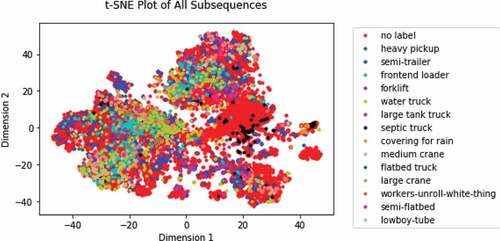
Figure 3 shows the t-SNE plot of all 14,000 segments from the six sequential days of seismic data. We can see concentrated areas of water truck, frontend loader and semi-trailer segments, but there are few visually distinguishable clusters in this data. Many areas are dominated by points with no label. The result suggests the framework may be overwhelmed by the number of activity types and the degree to which they may overlap or the features may not be sufficient for so many different activity types. The experiments that follow reduce the number of activity types down to two in an effort to determine the extent to which our approach can distinguish among smaller numbers of activities and types of activities. The reduction in the number of segments being clustered is comparable to real-world deployment, where the framework could be used to cluster segments from a time period of only a few hours or less.

Figure 3. T-SNE plot of all activities.

Evaluation Criteria

In a real-world PoL scenario, little to nothing is known about when or what activities are happening onsite. Instead, clusters can be trusted to correlate to onsite activities. To evaluate performance, we measure the purity, statistically analyze, and visually inspect each cluster to draw conclusions about performance.

The purity of a cluster is the percentage of the most common ground truth label within a cluster and is a good indicator of a specific activity type is separated from another. In a best-case scenario, each cluster would be 100% pure. To determine if a single cluster has high purity, its purity is compared to the overall purity of the data. We are not concerned with identical ground truth labels clustering into several separate clusters. Segments with the same ground truth label may easily form several clusters depending on the vehicle operations. For example, the seismic activity of a large crane moving onsite likely differs from its seismic activity when stationary and raising its arm. An activity type with most clusters having purity above the overall purity is a strong indicator that our framework is able to cluster segments from that activity type for further PoL analysis. An activity type with impure clusters suggests a lack of separation due either to activities being too similar or the preprocessing and feature extraction methodology being inadequate.

The statistical analysis gives us a probability of a cluster being random or not. This probability is calculated by viewing the clusters as samples without replacement from the population (all segments involved in an experiment). The motivation for using this statistical analysis is due to the imbalance of ground truth labels in our data, making evaluation of some clusters difficult when only examining the purity. In the context of clustering exactly two activity types in an experiment, this probability is formally known as a hypergeometric probability. The probability is defined as Equation (3)(3) $P(x,n,M,N)=\frac{\left(\begin{array}{c}M\\ x\end{array}\right)\left(\begin{array}{c}N-M\\ n-x\end{array}\right)}{\left(\begin{array}{c}N\\ n\end{array}\right)}$(3) , where $x$ is the number ground truth labels from one activity type within the cluster, $n$ is the size of the cluster, $M$ is the overall number of ground truth labels associated with $x$, and $N$ is the total number of all ground truth labels. We consider the possibility of a cluster being random when its probability is greater than 0.05.

(3) $P(x,n,M,N)=\frac{\left(\begin{array}{c}M\\ x\end{array}\right)\left(\begin{array}{c}N-M\\ n-x\end{array}\right)}{\left(\begin{array}{c}N\\ n\end{array}\right)}$(3)

We also rely on visual inspection of the individual clusters to make final conclusions about performance. Clusters with equal distribution of ground truth labels suggest that the framework is failing to capture features unique to onsite activity or that the seismic signals of the activities are too similar. This suggests that an entirely new approach for automatic detection and classification of onsite activities is needed or that the task itself is impossible due to the inherent problems arising from working with seismic sensors. Impure clusters with concentrated regions of ground truth labels suggest feature extraction is capturing signals unique to onsite activity, but overall, these clusters are determined by other signatures in the seismic data. Better data preprocessing or feature extraction could help improve clustering.

Experiments

We want to test the capability of our framework to successfully cluster two vastly different onsite activities. Figure 4 shows the t-SNE plot of segments corresponding to the large crane and covering for rain. There are 245 segments in total, with 226 from the large crane and 19 from the covering for rain. The large crane is the largest vehicle in operation at the construction site, powered by a diesel engine, moves on wide tracks, and generates substantial seismic activity. The covering for rain activity is mainly used ofor small gasoline vehicles, workers moving onsite, and generating little seismic activity.

Figure 4. T-SNE Plot of Covering for Rain and Large Crane.

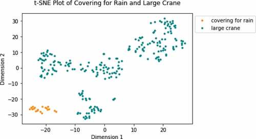
Since these are only pilot experiments, the selection of the number of clusters is based on visual inspection of the t-SNE plot. However, this selection is consistent with what formal metrics would suggest, as discussed in Section 6. Based on the visual inspection of Figure 4 we set the number of clusters to five. The overall purity of the data is 92.8%. Table 3 and Figure 5 show all five clusters are 100% pure with low probability, especially cluster 4. This experiment shows that our framework can easily distinguish between onsite activities when clustering on smaller subsets of the data that correspond to segments of seismic data from vastly different onsite activities.

Table 3. Statistics of Figure 5 GMM clustering assignments.

Cluster	Majority	Covering for Rain	Large Crane	Cluster	Hypergeometric
	activity	Count	Count	Purity	Probability
0	Large Crane	0	38	100.0%	$3.6\times {10}^{-2}$
1	Large Crane	0	49	100.0%	$1.2\times {10}^{-2}$
2	Large Crane	0	51	100.0%	$1.0\times {10}^{-2}$
3	Large Crane	0	88	100.0%	$1.4\times {10}^{-4}$
4	Covering for Rain	19	0	100.0%	$1.0\times {10}^{-28}$

Figure 5. GMM Clustering of Covering for Rain and Large Crane.

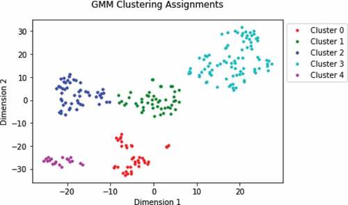
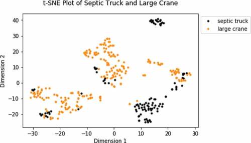
We want to test the capability of our framework to successfully cluster on two vehicles differently in terms of both size and onsite uses. Figure 6 shows the t-SNE plot of seismic segments corresponding to the large crane and septic truck. There are 337 segments in total, with 226 segments from the large crane and 111 seismic segments from the septic truck. The septic truck is relatively much smaller than the large crane and drives on four wheels, but is also powered by a diesel engine. We can expect the seismic activity of these two vehicles to be fairly different from each other.

Figure 6. T-SNE Plot of Septic Truck and Large Crane.

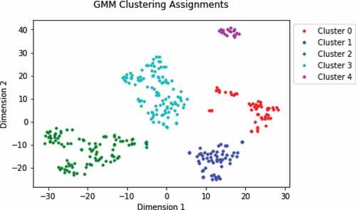
Based on visual inspection of Figure 6 the number of clusters is set to five. The overall purity of the data is 67.1%. Table 4 and Figure 7 show clusters with high purity and low probability for both activity types as seen in clusters 1 and 4 for septic truck and clusters 2 and 3 for large crane. However, cluster 0 has a relatively low purity compared to the other clusters and a probability low enough that indicates it might have formed due to random chance. Despite cluster 0, we consider this experiment a success for our framework because clusters with high purity and low probability were achieved for both activity types.

Table 4. Statistics of Figure 7 GMM clustering assignments.

Cluster	Majority	Septic Truck	Large Crane	Cluster	Hypergeometric
	activity	Count	Count	Purity	Probability
0	Large Crane	13	38	74.5%	$6.3\times {10}^{-2}$
1	Septic Truck	54	3	94.7%	$1.9\times {10}^{-27}$
2	Large Crane	15	88	85.4%	$5.2\times {10}^{-7}$
3	Large Crane	11	97	89.8%	$9.6\times {10}^{-11}$
4	Septic Truck	18	0	100.0%	$7.7\times {10}^{-10}$

Figure 7. GMM Clustering of Septic Truck and Large Crane.

We want to test the capability of our framework to successfully cluster two similarly sized and powered vehicles but used for very different tasks. Figure 8 shows the t-SNE plot of seismic segments corresponding to the large crane and frontend loader. There are 1,098 seismic segments in total, including 226 from the large crane and 872 from the frontend loader. The frontend loader, like the crane, is a large vehicle powered by a diesel engine but moves on tires instead of tracks. These vehicles perform very different tasks on the construction site. The large crane is responsible for lifting and moving heavy materials into place. The frontend loader is typically used to move gravel and dirt. Although the two vehicles operate differently onsite, their seismic waves may share similar characteristics due to their similar size and engine type.

Figure 8. T-SNE Plot of Frontend Loader and Large Crane.

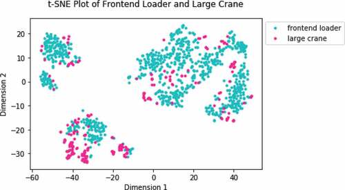
Based on visual inspection of Figure 8 the number of clusters is set to three. The overall purity of the data is 79.4%. Table 5 and Figure 9 show clusters with high purity and low probability for the frontend loader. However, cluster 2 is much more mixed, containing many segments from the frontend loader and most of the segments from the large crane. Despite the impurity of cluster 2, its probability is extremely low, indicating that the cluster is not random and our framework is separating based on extracted features from the onsite activities. This claim is also supported by visual inspection of cluster where concentrated regions of large crane can be seen. Note that highly pure clusters for both activities could be achieved if the number of clusters was increased to match what is suggested when including the small clusters seen in Figure 8 (approximately eight). Because the majority of segments from the frontend loader separate into their own clusters, and the probability along with visual inspection of cluster 2 indicate that our framework is achieving some level of separation, we believe this experiment is still an acceptable demonstration of our framework. This experiment suggests our framework is finding at least some signatures unique to the two onsite activities despite their similarity and the noise inherit in the seismic data. Better preprocessing or feature extraction could achieve better results.

Table 5. Statistics of Figure 9 GMM clustering assignments.

Cluster	Majority	Frontend Loader	Large Crane	Cluster	Hypergeometric
	activity	Count	Count	Purity	Probability
0	Frontend Loader	161	20	88.9%	$1.1\times {10}^{-4}$
1	Frontend Loader	597	86	87.4%	$1.9\times {10}^{-4}$
2	Large Crane	114	120	51.3%	$3.3\times {10}^{-34}$

Figure 9. GMM Clustering of Frontend Loader and Large Crane.

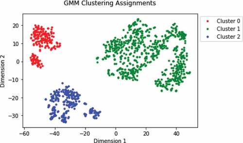
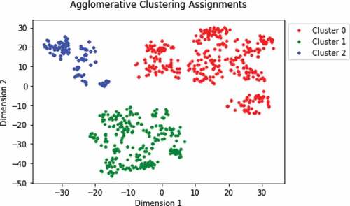
Finally, we want to test the capability of our framework to successfully cluster two almost identical activities. Figure 10 shows the t-SNE plot of seismic segments corresponding to the semi-trailer and semi-flatbed. There are 770 segments in total, including 708 segments from the semi-trailer and 62 from the semi-flatbed. The semi-trailer and semi-flatbed are both 18-wheeled vehicles, powered by a diesel engine and used for bringing supplies into the construction site. The main difference between both vehicles is the type of container hitched to their back. Because the vehicles are very similar, their corresponding seismic features may be nearly indistinguishable.

Figure 10. T-SNE Plot of Semi-trailer and Semi-flatbed.

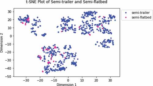
Based on visual inspection of Figure 10 we set the number of clusters to three. Table 6 and Figure 11 show that each cluster is dominated by a semi-trailer class but contains segments from both classes of semi. The overall purity of the data is 91.9%. Cluster 2 has similar purity but clusters 0 and 1 vary slightly. The probabilities of cluster 0 and 1 are also low, indicating that this discrepancy is not by chance. However, visual inspection of Figure 11 shows no concentration of a particular activity within these clusters. This experiment demonstrates the limitations of our framework finding separation in two very similar onsite activities.

Table 6. Statistics of Figure 11 GMM clustering assignments.

Cluster	Majority	Semi-Trailer	Semi-Flatbed	Cluster	Hypergeometric
	activity	Count	Count	Purity	Probability
0	Semi-Trailer	364	14	96.3%	$5.6\times {10}^{-6}$
1	Semi-Trailer	244	36	87.1%	$1.5\times {10}^{-4}$
2	Semi-Trailer	100	12	89.3%	$7.5\times {10}^{-2}$

Figure 11. GMM Clustering of Semi-trailer and Semi-flatbed.

Discussion

Our experiments show that the proposed framework constructs high-purity clusters in most subsets of the data. Even when data derives from similarly sized and powered vehicles, the results still suggest clusters are being determined by features from the onsite activity and not the inherent noise from using seismic sensors. An incremental clustering approach in a full-scale PoL analysis may therefore be viable. For example, imagine clustering on segments for every two to three hours of data to keep the number of segments low and the number of possible activities during the time period low. This approach would need to recognize similar clusters among the clustering increments to provide consistency across different time windows.

More research is needed to understand how well our framework will perform when clustering segments from more than two activities. Experimentation is needed to understand how many, and which types of activities introduce too much variation and cause clusters to merge and become indistinguishable. There are many different vehicles and actions performed on-site, and some actions can be performed by more than one vehicle. For example, both the large crane and the small crane may lift material. Because there are dozens of combinations of activities, these vehicles and actions should be categorized intentionally and strategically to determine the limitations of our framework in clustering more than two activities.

A variety of metrics were tested to determine the number of clusters, $k$, in our experiments. These metrics include: elbow plot analysis, silhouette score, Gap statistic (Tibshirani, Walther, and Hastie 2001), and Bayesian Information Criterion (BIC) (Watanabe 2013). In general, these metrics are calculated within cluster variation, between cluster variation, or both in some way. When applied to the principal components of the two t-SNE features, these metrics typically suggest the same $k$ indicated by counting the most prominent clusters in the t-SNE plot. However, analysis of the silhouette scores, using agglomerative clustering of either principal component or t-SNE features, tended to suggest a larger $k$ than other metrics. For example, silhouette score analysis suggested seven or eight clusters for the large crane and frontend loader experiment, leading to much better results for either agglomerative or GMM clustering. More experimentation to determine the reliability and specifics of how to select $k$ based this analysis is needed.

Additional research is also needed to understand why specific activities may be associated with two or more clusters and how this would affect downstream PoL analysis. To some degree, fracturing of a single activity into multiple clusters is expected (Ackerman and Dasgupta 2014), but we need to determine the specific cause. If association of a single activity with two or more clusters is caused by varying levels of noise, then further preprocessing or different methods of feature extraction should be considered. If instead this association is caused by differences in the operation of these vehicles or differences in their location relative to the sensor, then the cluster fragmentation may be irreducible and require another layer of analysis. In the latter case, study of the framework’s clustering fragmentation in response to changes in sensor location may help determine optimal sensor placement around a site under surveillance.

One of the biggest challenges with incorporating seismic sensors into PoL analysis is the amount of noise in the seismic data. Initial tests showed that quality of clusters were greatly affected by wavelet denoising or bandpass filtering in our framework. Exploration of other techniques used in signal processing for denoising, along with hyper-parameter tuning within current methods could help improve results. More generally, we anticipate that background noise and other sources of variation will be a common problem in pattern-of-life modeling. The challenge is that every combination of sensor, activity, and environment may require its own specialized approach to cleaning up the data. A better approach to separating on-site from off-site seismic activity may be to use three or more sensors to trigulate the coordinates of its origin. Experimentation is needed to determine the viability of this method is for filtering out off-site activity.

Another aspect of seismic data in PoL analysis worth understanding is the effect of distance from seismic sensor to entity. Currently, only one seismic sensor located 500 m from the center of the construction site was used in our analysis. Experiments to understand how segment clusters change based on sensor distance and incorporation of sensors of varying distances is vital to understand a full-scale PoL analysis framework. Likewise, anecdotal evidence suggests that the velocity and direction of movement, at least for heavy equipment, also impacts the structure of the signals. A possible outcome from these experiments might show the need to accommodate multiple clusters for each activity based on distance, but also identify specific relationships among the cluster members.

There is also opportunity to develop the unsupervised machine learning framework for clustering seismic data to a semi-supervised method for refining ground truth. Given a set of ground truth labels that may only be an estimate of when activities are occurring, the framework can help pinpoint when activities actually begin and end. The framework can be used to cluster on much shorter one or two hour periods of time that contain ground truth, avoiding problems of overwhelming the framework with too many segments. Examination of the temporal proximity of unlabeled segments to labeled segments and when segments start forming different clusters, can help refine ground truth labels. For example, given a ground truth label of the large crane that says operation occurred from 09:00 to 09:15, we can use the unsupervised approach of the framework to cluster on the time period from 08:00 to 10:00 of the seismic data. The analysis might reveal that segments from 08:50 to 09:30 all fall into the same cluster, and due to their temporal proximity to the given label, the ground truth for the large crane operation can be extended to 08:50–09:30.

A long-term application of this research may include discovering broader underlying activities within the construction site. Our framework can correctly cluster the operation of individual equipment and vehicles, even in difficult scenarios. These individual operations can be mapped to longer processes happening on the construction site such as installing HVAC, laying foundation, or framing the building. For example, sudden regular detections of a cement truck could mark the start of a new phase in construction for laying the foundation of the building. Knowing which phase of construction we are in could help us limit which vehicles and equipment we want to detect and identify abnormal operations occurring on the construction site.

We have identified two clear next steps in developing data-driven methods for pattern-of-life activity analysis. One step is to use the clustering results described above to drive activity labeling. Ideally, we would be able to label various time periods in the data with the specific equipment that is active. Pilot experiments suggest that labeled data available from the time lapse camera is insufficient to train a labeling algorithm, so the goal is to leverage the unsupervised learning results to increase the amount of labeled training data in a semisupervised sense. The second step is to test our approach on a different construction site using a different arrangement of sensors, and detecting a different set of equipment and activities. Ideally, we should be able to follow the same set of steps described above and achieve similar clustering results. Subsequent steps include the many fine-tuning efforts described above, such as generalizing the clustering approach to work over long time periods, determining and addressing the cause of cluster fragmentation, and determining the degree to which sensor placement influences our detection and clustering results.

Conclusions

We introduced a new framework for automatically discovering activities from a region being monitored with seismic sensors. Our approach tested a variety of data cleaning, feature extraction, and unsupervised machine learning approaches that minimized prior assumptions about the activity of the region. The approach should therefore be applicable to other monitoring scenarios and possibly other time series datasets such as financial, social, or video. Importantly, other analytic contexts may require other combinations of the methods that we considered, so the evaluation process, based in our case on cluster purity for a known set of examples, is necessarily part of the approach. A variety of extensions to support analysis of higher-level patterns, such as anomaly detection, are also possible. Feature analysis reveals that features from the frequency domain capture the most variance from the seismic data. Future research into seismic feature extraction methods for PoL application should focus on extracting features from the frequency domain instead of the time–frequency domain. Our results are promising and provide insight for directions of future work.

Acknowledgments

The authors thank Nicole McMahon for providing the analysis to detect inactive segments of seismic activity. This work was funded by the U.S. Department of Energy National Nuclear Security Administration’s Office of Defense Nuclear Nonproliferation Research & Development (NA-22). Sandia National Laboratories is a multimission laboratory managed and operated by National Technology & Engineering Solutions of Sandia, LLC, a wholly owned subsidiary of Honeywell International Inc., for the U.S. Department of Energy’s National Nuclear Security Administration under contract DE-NA0003525.

Disclosure statement

No potential conflict of interest was reported by the author(s).

References

- Ackerman, M., and S. Dasgupta (2014). Incremental clustering: The case for extra clusters. In Proceedings of the 27th International Conference on Neural Information Processing Systems, Montreal Canada, pp. 307–2761.
- Adams, R. P., and D. J. MacKay (2007). Bayesian online changepoint detection. arXiv:0710.3742.
- Allen, R. 1982. Automatic phase pickers: Their present use and future prospects. Bulletin of the Seismological Society of America 72 (6B):S225–S242.
- Chamarczuk, M., Nishitsuji, Y., Malinowski, M., and Draganov, D. 2020. Unsupervised learning used in automatic detection and classification of ambient‐noise recordings from a large‐N array. Seismological Research Letters 91 (1):370–389.
- Craddock, R., D. Watson, and W. Saunders (2016). Generic pattern of life and behaviour analysis. In IEEE International Multi-Disciplinary Conference on Cognitive Methods in Situation Awareness and Decision Support (CogSIMA), San Diego, USA. IEEE Press.
- Ghosh, R., A. Akula, S. Kumar, and H. K. Sardana. 2015. Time–frequency analysis based robust vehicle detection using seismic sensor. Journal of Sound and Vibration 346:424–34.
- Ghosh, R., and Sardana, H. K. 2020, June. Multi-feature optimization strategies for target classification using seismic and acoustic signatures. In Automatic Target Recognition (Vol. 11394, p. 113940). International Society for Optics and Photonics.
- Huang, J., Q. Zhou, X. Zhang, E. Song, B. Li, and X. Yuan. 2013. Seismic target classification using a wavelet packet manifold in unattended ground sensors systems. Sensors 13 (7):8534–50. doi:10.3390/s130708534.
- Jin, X., S. Sarkar, A. Ray, S. Gupta, and T. Damarla. 2011. Target detection and classification using seismic and pir sensors. IEEE Sensors Journal 12 (6):1709–18.
- Johnson, S. C. 1967. Hierarchical clustering schemes. Psychometrika 32 (3):241–54. doi:10.1007/BF02289588.
- Johnson, C. W., Ben‐Zion, Y., Meng, H., and Vernon, F. 2020. Identifying different classes of seismic noise signals using unsupervised learning. Geophysical Research Letters 47(15):e2020GL088353.
- Kalra, M., S. Kumar, and B. Das. 2018. Target detection using smooth pseudo Wigner-Ville distribution. IEEE Recent Advances in Intelligent Computational Systems (RAICS), Thiruvananthapuram, India. IEEE Press, pp. 6-10.
- Kalra, M., S. Kumar, and B. Das. 2020. Seismic signal analysis using empirical wavelet transform for moving ground target detection and classification. IEEE Sensors Journal 20 (14):7886-7895.
- Killick, R., P. Fearnhead, and I. Eckley. 2012. Optimal detection of changepoints with a linear computational cost. Journal of the American Statistical Association 107 (500):1590–98.
- Lan, J., S. Nahavandi, T. Lan, and Y. Yin. 2005. Recognition of moving ground targets by measuring and processing seismic signal. Measurement 37 (2):189–99.
- Lloyd, S. P. 1982. Least squares quantization in PCM. IEEE Transactions on Information Theory 28 (2):129–37.
- McNamara, D. E., and R. Boaz. 2006. Seismic noise analysis system using power spectral density probability density functions: A stand-alone software package. Reston, Virginia: US Geological Survey: Citeseer.
- Moore, A. W. 1998. Very fast EM-based mixture model clustering using multiresolution kd-trees. Advances in Neural information processing systems, Denver, CO, USA.
- Ntalampiras, S. 2018. Moving vehicle classification using wireless acoustic sensor networks. IEEE Transactions on Emerging Topics in Computational Intelligence 2(2): 129–138.
- Riahi, N., and Gerstoft, P. 2017. Using graph clustering to locate sources within a dense sensor array. Signal Processing 132:110–120.
- Scott, A. J., and M. Knott. 1974. A cluster analysis method for grouping means in the analysis of variance. Biometrics 30:507–12.
- Snover, D. et al. 2021. Deep clustering to identify sources of urban seismic noise in Long Beach, California. Seismological Society of America 92(2A):1011–1022.
- Stephane, M. (1999). A wavelet tour of signal processing.
- Tian, Y., H. Qi, and X. Wang. 2002. Target detection and classification using seismic signal processing in unattended ground sensor systems. IEEE International Conference on Acoustics Speech and Signal Processing 4 :4172-4172.
- Tibshirani, R., G. Walther, and T. Hastie. 2001. Estimating the number of clusters in a data set via the gap statistic. Journal of the Royal Statistical Society. Series B, Statistical Methodology 63 (2):411–23.
- van der Maaten, L., and G. Hinton. 2008. Visualizing data using t-SNE. Journal of Machine Learning Research 9:2579–605.
- Vasco, D. W., J. E. Peterson Jr, and E. L. Majer. 1996. A simultaneous inversion of seismic traveltimes and amplitudes for velocity and attenuation. Geophysics 61 (6):1738–57.
- Watanabe, S. 2013. A widely applicable Bayesian information criterion. Journal of Machine Learning Research 14(Mar):867–97.
- Welch, P. 1967. The use of fast Fourier transforms for the estimation of power spectra: A method based on time averaging over short modified periodograms. IEEE Transactions on Audio and Electroacoustics 15:70–73.
- William, P. E., and M. W. Hoffman. 2011. Classification of military ground vehicles using time domain harmonics’ amplitudes. IEEE Transactions on Instrumentation and Measurement 60 (11):3720–31.
- Wold, S., K. Esbensen, and P. Geladi. 1987. Principal component analysis. Chemometrics and Intelligent Laboratory Systems 2 (1–3):37–52.