Smart Cities-Based Improving Atmospheric Particulate Matters Prediction Using Chi-Square Feature Selection Methods by Employing Machine Learning Techniques

ABSTRACT

Particulate matter is emitted from diverse sources and affect the human health very badly. Dust particles exposure from the stated environment can affect our heart and lungs very badly. The particle pollution exposure creates a variety of problems including nonfatal heart attacks, premature deaths in people with lung or heart disease, asthma, difficulty in breathing, etc. In this article, we developed an automated tool by computing multimodal features to capture the diverse dynamics of ambient particulate matter and then applied the Chi-square feature selection method to acquire the most relevant features. We also optimized parameters of robust machine learning algorithms to further improve the prediction performance such as Decision Tree, SVM with Linear and Regression, Naïve Bayes (NB), Random Forest (RF), Ensemble Classifier, K-Nearest Neighbor, and XGBoost for classification. The classification results with and without feature selection methods yielded the highest detection performance with random forest, and GBM yielded 100% of accuracy and AUC. The results revealed that the proposed methodology is more robust to provide an efficient system that will detect the particulate matters automatically and will help the individuals to improve their lifestyle and comfort. The concerned department can monitor the individual’s healthcare services and reduce the mortality risk

Introduction

Across the globe, the major source of pollutions is particulate matters (PMs), which severely affect the human health (Ostro, Broadwin, and Lipsett 2000; Weng, Chang, and Lee 2008). The PM particles range in size from a few nanometers to tens of micrometers (µm) in diameter, i.e., PM1.0, PM2.5, and PM10.0. The composition, size, and distribution of these particles affect the human health hazardously (Ostro, Broadwin, and Lipsett 2000). Human health has more impact on ultra- and fine particles (PM1.0 and PM2.5) as compared to the coarse particles (PM10) (Laden et al. 2014; Mar et al. 2006). According to the world bank estimate in 1993, there was about 50% of the disease due to the indoor particulate matter and poor household environment in developing countries (Albalak et al. 1999; L. P. Naeher et al. 2001).

In rural areas, people use the domestic wood combustion heaters, which contributes significantly to ambient PM in moderate or cold winters (Ancelet et al. 2013; Glasius et al. 2006; Grange et al. 2013; Molnár and Sallsten 2013; Trompetter et al. 2013). The exacerbations and respiratory symptoms, especially in the children and young adults, are associated with the elevated concentrations of the ambient PM in wood-burning communities (Lipsett, Hurley, and Ostro 1997; McGowan et al. 2002; Luke P. Naeher et al. 2007; Town 2001). The studies (Sarnat et al. 2008) show that wood combustion PM emission found daily wood smoke PM 2.5 to be associated with hospital emergency department visits for cardiovascular disease but not respiratory disease. The studies also reveal that wood smoke-affected people have similar magnitude to that of gasoline and diesel PM2.5.

The airborne particles (such as PM10 and PM2.5) have a pathophysiological influence on health in the form of inflammatory response and oxidative stress in the respiratory system along with consecutive systemic inflammatory responses (Annesi-Maesano et al. 2007; Portnov and Paz 2008; Schlesinger et al. 2006). The empirical studies (Y. S. Chen et al. 2004) in Taiwan reveal different health impacts due to dust storms, which increased the risk of respiratory diseases by 7.66% in one day after the event, 4.92% total deaths after two days, resulting in the dust storm, and 2.59% cardiovascular diseases in two days, leading to the dust storm. In recent years, the environmental changes occur due to soil degradation and desertification processes in parallel with changes in intensity and wind direction (Portnov and Paz 2008; Portnov, Paz, and Shai 2011).

Human health has a very bad impact from the particulate matters concentration emitted from diverse sources and indoor and outdoor sources. The particle pollution exposure creates a variety of problems including nonfatal heart attacks, premature deaths in people with lung or heart disease, aggravated asthma, irregular heartbeat, decreased lung function, increase in respiratory symptoms causing coughing and difficulty in breathing, etc. The concentration in PM time series can be of diverse nature comprising time variants (short-, medium-, and long-term variation) and nonlinear, nonstationary, and complex dynamics based on emitted concentrations of PM time series. Researchers recently emphasis only the classification of indoor and outdoor PM concentration time series. However, there is dire need to investigate these multiple dynamics present in particulate matter time series data by computing the associations and relationships among the extracted features. Moreover, we aim to develop the ranking algorithms to compute the feature importance that ranks the multimodal extracted features based on the feature importance. We further investigated the association and relationship among the features based on top ranked features. The proposed study can thus be utilized by environmental institutions and decision makers that which characteristics of PM concentrations can be of importance to make further decisions and awareness campaigns to reduce the risks produced due to the PM time series data. Based on the outcomes, we will provide the mechanism to control, monitor, and reduce the effects of these pollutants to the concerned Government department for policy making and awareness.

This study is aimed to predict the particulate time series by extracting multimodal features from time-domain (to capture the short-, medium-, and long-term variations), statistical features (to capture statistical variations), and entropy-based complexity measures (to capture the nonlinear, non-stationary, and highly complex dynamics) present in the particulate matter time series from both indoor and outdoor selected at different locations of Muzaffarabad, Azad Kashmir, Pakistan, with and without feature selection methods. We then optimized and employed robust machine learning techniques such as decision tree (DT), k-nearest neighbour (KNN), support vector machine -linear & radial based kernel (SVM-L & R), naïve bayes (NB), eXtreme boosting linear and tree (XGB-L, XGB-T), and average neural network (AVNNET). The proposed methods yielded the higher prediction results.

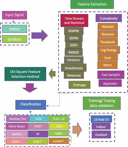
Figure 1 reflects the schematic diagram to predict the particulate matter. In the first step, we extracted the time-domain, statistical (to capture short, medium and long variations) features, wavelet, and entropy-based complexity features (to capture the nonlinear dynamics) from indoor and outdoor particulate time series data. We optimized the parameters of machine learning algorithms. We then fed these features with and without feature selection method as input to supervised machine learning algorithms including decision tree, KNN, SVM-L, SVM-T, Naïve bayes, NNET, LVQ, AMDAI, RF< GBM, XGB-L, XGB-T, AVNNET. The 10-fold cross-validation was used for training and testing data validation. The proposed approach yielded the improved prediction results.

Figure 1. Schematic diagram to detect particulate matter (PM).

Materials and Methods

The current study was performed in the main campus of University of Azad Jammu and Kashmir (UAJK), which is a public sector university of AJ&K recognized back in the year 1980 and is multicampus and multidiscipline. The University is located at Muzaffarabad, which is the capital of Kashmir, that is ruled by Pakistan, and it is also known as Azad Jammu and Kashmir (AJ&K). Muzaffarabad is a lovely valley in the form of a cup. At the convergence of the Neelum and Jhelum streams, the city is located at 73.47 E (Longitude) and 34.37 N (Latitude). River Neelum divides the university into campuses, which are namely called City campus and Chehla campus.

Data Acquisition

Particulate Matter (PM_2.5) concentrations were collected from the main campus of University of Azad Jammu and Kashmir, which is located at the roadside, leading from Combined Military Hospital (CMH) to upper Addah, of Muzaffarabad. Each of the values of indoor and outdoor at specific locations are averages of 21,600 data points. The mean concentrations of ambient indoor and outdoor PM at different selected sites of Muzaffarabad city and training times are detailed in Hussain et al. (2020a). Data were collected using “Environmental Particulate Air Monitor (EPAM-5000), Haz-Dust,” which is a sensitive and precise instrument for ambient, air quality investigations, environmental monitoring, and baseline surveys (“SKC Ltd. Unit 11, Sunrise Business Park Higher Shaftesbury Road Blandford Forum Dorset DT11 8ST UK) (https://www.skcltd.com/products-category/90-particulatesampling/348-epam5000-mainpage-6”).

Its working principle uses the near-forward light scattering method of infrared radiations from the particles and thereby continuous measurement of their concentrations. The instrument records real-time airborne particle concentration data in mg/m³. Based upon interchangeable size-selective impactors, the instrument measures particulate matters with different sizes, viz., PM₁₀, PM_2.5, and PM_1.0. The instrument can sample for up to 24 hours on one battery, and monitoring data can be stored up to 15 months. Using DustComm Pro Software, the data can be downloaded and stored on the computer for analysis purposes. At each site, EPAM-5000 was installed for consecutive six hours in the closed location to monitor the concentration of indoor particulate matter at a sampling rate of one second that will generate 21600 samples for each reading of six hours. Data collection was made for consecutive 26 days. After acquiring the data, the data were transferred to a personal computer with the help of manufacturer provided software, i.e., DustComm Pro Software.

Features Extraction

Features extraction is one of the most important steps before applying the Machine Learning and Neural networks classification techniques for detection and prediction purposes. It requires an optimum feature set that should effectively discriminate the subjects. Features extraction is solely specific to the problem. Ferland et al. (2017) and Rathore et al. (2014) extracted hybrid and geometric features for automatic colon detection of cancer. Dheeba, Albert Singh, and Tamil Selvi (2014) extracted texture features for breast cancer detection. Hussain et al. (2014) computed texture and morphological features to detect and classify the human face from nonfaces. Moreover, Hussain et al. (2017b) recently extracted acoustic features such as volume and pitch and prosodic features such as frequency minimum, maximum, sum, and Mel frequency cepstral coefficients for emotion recognition in human speech. They also extracted time and frequency-based features for detecting the heart rate and heart rate variability.

However, few studies (L. Wang et al. 2017) suggest the use of multimodal features, i.e., combing features from multidomains along with the nonlinear features for classifying the epileptic seizure. This will give a unified framework to include the advantages of varying characteristics of EEG signals. In this study, we have also extracted the features based on the time-domain, frequency domain, complexity-based measures, and wavelet entropy methods for classifying the epileptic seizure subjects from healthy subjects and postictal heart rate oscillations. Apart from this, in this work, we extracted nonlinear features using sample entropy based on the KD tree algorithmic approach (fast sample entropy) and approximate entropy, which gives outer performance than the results obtained by L. Wang et al. (2017) and is consistent with the results obtained by (Hussain et al. 2017a). Recently, Pan et al. and Hussain et al. (Hussain et al. 2017a; Pan et al. 2011) employed fast MSE, which gives statistically more effective results than traditional MSE with reduced computational and memory complexity.

We utilized different variants of entropy features as detailed below to capture multiple dynamics present in PM time series concentration data.

Time-Domain Analysis

To calculate the time variability in PM time series signals, time-domain features are derived in various ways.

SDSD: In each time series section, the difference between adjacent intervals’ standard deviation is measured.

SDNN: by calculating the standard deviation of each segment’s PM intervals,

(1) $\mathrm{S}\mathrm{D}\mathrm{P}\mathrm{M}=\sqrt{\frac{1}{\mathrm{N}-1}{\mathrm{\Sigma }}_{\mathrm{j}=1}^{\mathrm{N}}{(\mathrm{P}{\mathrm{M}}_{\mathrm{j}}-\overline{\mathrm{P}\mathrm{M}})}^2}.$(1)

RMSSD: The root square of the mean squared difference of N consecutive PM intervals was calculated,

(2) $\mathrm{R}\mathrm{M}\mathrm{S}\mathrm{S}\mathrm{D}=\sqrt{\frac{1}{\mathrm{N}-1}{\mathrm{\Sigma }}_{\mathrm{j}=1}^{\mathrm{N}-1}{(\mathrm{P}{\mathrm{M}}_{\mathrm{j}+1^{-}}\mathrm{P}\mathrm{M})}^2}.$(2)

SDAPM: For averages of PM intervals, the standard deviation is calculated,

$\mathrm{S}\mathrm{D}\mathrm{A}\mathrm{P}\mathrm{M}=\mathrm{S}\mathrm{D}[\mathrm{u}1,\mathrm{u}2,\mathrm{u}3,\mathrm{u}4,\dots ..\mathrm{u}\mathrm{n}].$

Nonlinear Methods

Biological signals are the complicated patterns generated by multiple interacting components of a biological system. These patterns of change may reveal valuable knowledge about these systems’ dynamics. Using conventional data analysis methods to obtain useful information is impractical. The most widely used difficulty base measures are listed below.

Entropy-Based Features

EEG signals have nonlinearity, which means that they contain hidden information about their dynamics. Information theoretical methods based on entropy are the most widely used for signal analysis since traditional approaches to collecting useful information are impractical.

Approximate Entropy

Pincus introduced approximate entropy (ApEn) in 1991 as a statistical measure for calculating data regularities. ApEn shows that identical patterns are not replicated by computing the likelihood,

(3) $ApEn(m,r.N)={\varphi }^{\mathrm{m}}(\mathrm{r})-{\varphi }^{\mathrm{m}+1}(\mathrm{r}).$(3)

Fast Sample Entropy with the KD Tree Approach

Costa (2002) suggested the sample entropy (SampEn), and ApEn has been changed in this edition. SampEn is a time series physiology measurement tool. It is also independent of data length and can be calculated using the following formula:

(4) $\mathrm{S}\mathrm{a}\mathrm{m}\mathrm{p}\mathrm{E}\mathrm{n}(\mathrm{m},\mathrm{r})=\underset{\mathrm{N}\to \mathrm{\infty }}{\mathrm{l}\mathrm{i}\mathrm{m}}-\mathrm{I}\mathrm{n}\frac{\mathrm{P}{\mathrm{m}}_{(\mathrm{r})}}{\mathrm{Q}{\mathrm{m}}_{(\mathrm{r})}}.$(4)

Self-matches are excluded, Pm (r) denotes the probability that two sequences will match for m + 1 points, and Qm (r) denotes the probability that two sequences will match for m points (with a tolerance of). Equation 4(4) $\mathrm{S}\mathrm{a}\mathrm{m}\mathrm{p}\mathrm{E}\mathrm{n}(\mathrm{m},\mathrm{r})=\underset{\mathrm{N}\to \mathrm{\infty }}{\mathrm{l}\mathrm{i}\mathrm{m}}-\mathrm{I}\mathrm{n}\frac{\mathrm{P}{\mathrm{m}}_{(\mathrm{r})}}{\mathrm{Q}{\mathrm{m}}_{(\mathrm{r})}}.$(4) can be written as follows in this case:

(5) $\mathrm{S}\mathrm{a}\mathrm{m}\mathrm{p}\mathrm{E}\mathrm{n}(\mathrm{m},\mathrm{r},\mathrm{N})=-\mathrm{I}\mathrm{n}\frac{\mathrm{P}{\mathrm{m}}_{(\mathrm{r})}}{\mathrm{Q}{\mathrm{m}}_{(\mathrm{r})}}.$(5)

By setting

(6) $Q=\{\frac{[(\mathrm{N}-\mathrm{m}-1)(\mathrm{N}-\mathrm{m})]}{2}\}{\mathrm{Q}}^{\mathrm{m}}(\mathrm{r})andP=\{\frac{[(\mathrm{N}-\mathrm{m}-1)(\mathrm{N}-\mathrm{m})]}{2}\}{\mathrm{P}}^{\mathrm{m}}(\mathrm{r}),$(6)

we have $\frac{\mathrm{p}}{\mathrm{Q}}=\frac{{\mathrm{P}}^{\mathrm{m}}\left(\mathrm{r}\right)}{{\theta }^{\mathrm{m}}\left(\mathrm{r}\right)}$, and as a result, sample entropy can be written as

(7) $\mathrm{S}\mathrm{a}\mathrm{m}\mathrm{p}\mathrm{E}\mathrm{n}(\mathrm{m},\mathrm{r},\mathrm{N})=\frac{P^m(r)}{Q^m(r)},$(7)

where P is the total number of forward matches of length m + 1 and Q is the total number of templates matches of length m. Here, we used sample entropy with the KD tree algorithmic base approach as implemented by Hussain et al. (2017a), which provides improved performance and is more effective with respective to time and space complexity.

Wavelet Entropy

Nonlinearity in a time series can also be calculated using wavelet entropy methods. Log Energy, Shannon, Threshold, Norm, and Sure are some of the most widely used wavelet methods (Lu et al. 2018). The Shannon entropy (D. Wang, Miao, and Xie 2011) was used to determine the signal to wavelet coefficient complexity produced by the wavelet packet, with larger values indicating greater complexity. Wavelet entropy used by Rosso et al. (2001) provided the useful information to measure the underlying dynamical process associated with the signal. The entropy ‘E’ must be an additive information cost function, as shown below:

(8) $\mathrm{E}(0)=0\mathrm{a}\mathrm{n}\mathrm{d}\mathrm{E}(\mathrm{s})={\mathrm{\Sigma }}_{\mathrm{i}}\mathrm{E}({\mathrm{s}}_{\mathrm{i}}).$(8)

Shannon Entropy

Claude proposed Shannon entropy in 1948, as presented by Wu et al. (2013). Shannon’s entropy has been commonly used in various areas of information processing systems since then. It is a measure for estimating a random variable’s degree of uncertainty. It establishes the expected value of the data found in a particular message. The Shannon entropy of variable X can be expressed mathematically as follows:

(9) $V(X)=V(P_1,\dots \dots ..,P_n,)=-\sum _{i=1}^n{P}_{i}lo{g}_2{P}_i,$(9)

(10) $P_i=P_r(X=x_i).$(10)

In the above equation, Pi is defined, with $x_i$ indicating the ith possible value of X out of n symbols and Pi denoting the possibility of $X=x_i$.

Wavelet Norm Entropy

The Wavelet Norm entropy (Avci, Hanbay, and Varol 2007) is defined as

(11) $\mathrm{E}(\mathrm{S})=\frac{\sum _{\mathrm{i}}|{\mathrm{S}}_{\mathrm{i}}{|}^{\mathrm{p}}}{\mathrm{N}},$(11)

where p is the power and must be $1\ll \mathrm{P}<2$ the terminal node signal and (S_i) i the waveform of terminal.

Feature Selection

In the machine learning, one of the most important steps is to extract the most relevant features, which could improve the detection performance. Researchers have emphasized to propose a variety of different feature extracting strategies for features extraction based on the type and nature of problem. All the extracted features are not important, which may contribute to proper identification. So, feature selection (also known as attribute selection) is a method of selecting those important attributes, which contain necessary/relevant information in the dataset (Zhao and Liu 2007). This method is very handy when extracting relevant variables from the high-dimensional dataset, which contains redundant, useless, or irrelevant features (Yu and Liu 2003). Feature selection needs to be performed only once, and then different classifiers can be evaluated (Saeys, Inza, and Larranaga 2007). There are four main advantages of feature selection techniques, and it improves the model’s training time because the subset of variables takes less memory and computational time for a model (Kohavi and John 1997), improves generalization by reducing variance, avoids curse of dimensionality, and simplifies the model. The chi-square test can be used to select important features from the high-dimensional data set (Jin et al. 2006). Recently, researchers have been utilizing the feature selection algorithms to improve the prediction performance. Rostami et al. (2022) applied the gene selection algorithm to improve the classification accuracy of microarray data. Rostami, Berahmand, and Forouzandeh (2021) also applied genetic algorithm-based feature selection methods for improved community detection problems. Saberi-Movahed et al. (2021) utilized the feature selection method to decode clinical biomarker space of COVID-19. Rostami et al. (2021) recently comprehensively reviewed the different features selection methods applied on various problems analysis for improved performance measure. Mostly, the high-dimensional data usually have a lot of features, which becomes a hard learning task for classifiers. Moreover, the deep learning CNN methods compute many features. In this study, we extracted 2048 features from the FC layer of ResNet101 from multiclass (COVID-19, normal, bacterial, and viral pneumonia). Dimensionality reduction by applying the appropriate feature selection approach helps to reduce the number of variables of high-dimensional data by discarding the less informative variables and ensure similar information. We utilized the chi-square feature selection algorithm. The chi-square feature selection algorithm is successfully been utilized in many recent problems for prediction and classification (Cai, Shu, and Shi 2021; Rosidin et al. 2021; Shrestha et al. 2021). In this case, nonparametric chi-square methods chosen are not based on assumptions and the sample collected also does not follow the specific distribution. The chi-square feature selection algorithm for feature selections from multimodal features computed from particulate matters time series is detailed in the below section:

Chi-Square Feature Selection

It is the most simple and general feature selection algorithm in which a${ }^2$ value is repeatedly selected to determine the intervals of a numeric attribute. After extracting the features, these are selected based on the characteristics of the data. The chi-square algorithm has two significant levels, which are based on the $X^2$ value. The first step is the high significance level (sigLevel), which is computed for all numeric attributes for discretization. After sorting each of the attribute according to its type, the following procedure is performed:

1. The $X^2$ value for every pair of closest intervals is calculated.

2. The adjacent interval pairs are merged with the lowest $X^2$ value, and this process continues as long as all pairs of intervals contain $X^2$ values, which are greater than the parameter determined by sigLevel.

The above process is repeated with a decreased sigLevel until an inconsistency rate ($\delta$), ‘incon ()’, is exceeded in the discretized data. The chi-square ($X^2$) is computed using the following equation:

(12) $X^2=\sum _{i=1}^2\sum _{j=1}^k\frac{{(A_{ij-E_{ij}})}^2}{E_{ij}},$(12)

where

• k = number of (No.) classes,

• $A_{ij}$= No. of patterns in the ith interval, jth class,

• $E_{ij}$= expected frequency of Aij = Ri* C j/N,

• $R_i$= No. of patterns in the ith interval,

• $C_j$= No. of patterns in the jth class,

• N = total No. of patterns.

Classification

We applied and compared 09 supervised machine learning classification algorithms: CART, KNN, SVM-L, SVM-R, NB, GBM, XGB-L, XGB-T, and AVNNET methods. In machine learning, ensemble is the collection of multiple models and is one of the self-efficient methods as compared to other basic models. The ensemble technique combines different hypotheses to hopefully provide best hypothesis. Basically, this method is used for obtaining a strong learner with the help of combination of weak learners Experimentally, ensemble methods provide more accurate results even when there is considerable diversity between the models. Boosting is a most common type of ensemble method that works by discovering many weak classification rules using the subset of training examples simply by sampling again and again from the distribution. The summary of robust machine learning algorithms with parameter optimization is enlisted below:

Support Vector Machine (SVM)

For supervised learning methods, SVM is one of the most robust methods used for classification purposes. Recently, SVM was excellently used for pattern recognition problems (Vapnik 1999), machine learning (Gammerman et al. 2016), and medical diagnosis area (Dobrowolski, Wierzbowski, and Tomczykiewicz 2012; Subasi 2013). Moreover, SVM is used in a variety of applications such as recognition and detection, text recognition, content-based image retrial, biometrics, speech recognition, etc. SVM construct a hyperplane or set of hyperplanes in infinite or high dimensional space using kernel trick to separate the nonlinear data with larger margin. The good classification separation is achieved with larger margin, which indicates the lower generalization error of the classifier. SVM tries to find a hyperplane that gives the largest minimum distance to the training example. In SVM theory, this name is also known as margin. For the maximized hyperplane, the optimal margin is obtained. SVM has another important characteristic that gives the greater generalization performance. SVM is basically, a two-category classifier, which transformed data into a hyperplane depending on the nonlinear training data or higher dimension.

For explaining ambiguity in SVM, we take a binary classification problem where classes can separate linearly. Consider a data set D with classes $\left(C1,Y1\right),\left(C2,Y2\right),\dots \dots ,\left(Ci,Yi\right)$. Here, $Yi$ are training tuples and associated class labels $Yi$, in which each $Yi$ contains only one value, for example, can buy a computer or not. In Fig 1 and 2, graphs show the linear separation of data in 2-dimension, a plane for 3-dimension, and a hyperplane for n dimensions, here a straight-line separates class +1 tuple from class −1. Several infinite straight lines could be drawn for the separation of tuples from two classes. The problem is to find the best line, plane, or hyperplane that has a minimum error in classification for unseen tuples.

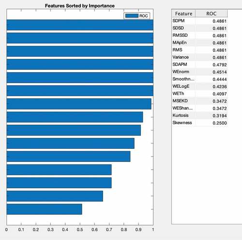
Figure 2. Multimodal features ranking.

The SVM technique is used to find the maximum marginal hyperplane for solving a problem. Figure 1 shows two separating hyperplanes and related margin lines, and we suppose that after classification, the accurate result can be obtained with a larger margin as compared to smaller. That is why during the training phase, SVM searches for hyperplanes with a maximum margin. The equation for finding a hyperplane is

(13) $\mathit{W}.\mathit{X}+\mathit{b}=0.$(13)

Here, w represents the weight vector, W₁, W₂, … ., W_n represent No. of attributes, and b is scalar called bias.

Margins of hyperplane can be defined by adjusting the weights as below:

${\mathit{w}}_0+{\mathit{w}}_1{\mathit{x}}_1+{\mathit{w}}_2{\mathit{x}}_2>0,$

(14) ${\mathit{w}}_0+{\mathit{w}}_1{\mathit{x}}_1+{\mathit{w}}_2{\mathit{x}}_2<0.$(14)

The weights can be adjusted so that the hyperplanes defining the “sides” of the margin can be written as

(15) $\begin{array}{c}\mathit{H}1:{\mathit{w}}_0+{\mathit{w}}_1{\mathit{x}}_1+{\mathit{w}}_2{\mathit{x}}_2\ge 1\mathit{f}\mathit{o}\mathit{r}{c}_{\mathit{i}}=+1,\\ \mathit{H}2:{\mathit{w}}_0+{\mathit{w}}_1{\mathit{x}}_1+{\mathit{w}}_2{\mathit{x}}_2\le 1\mathit{f}\mathit{o}\mathit{r}{c}_{\mathit{i}}=-1.\end{array}$(15)

According to it, if tuples lying above H1 belong to class +1 whereas, in other cases, it belongs to class −1.

The SVM classification algorithm performance can be further improved by optimizing several parameters. In this study, we optimized the parameters using the grid search algorithm (Rathore, Hussain, and Khan 2015) by carefully setting the grid range and step size. For linear kernel, the parameter ‘c’ is used, which constrains violation cost associated with the data point occurring on the wrong side of the decision surface. For RBF kernel, the value of gamma is important. We adjusted the following parameters for optimization of parameters:

param_grid = {‘C’: [0.1,1, 10, 100], ‘gamma’: [1,0.1,0.01,0.001],’kernel’: [‘rbf’].

Random Forest

Random forest is another type of machine learning classifier, which is operated by constructing an assembly of decision trees. The result is achieved by averaging the output founded from all DTs. (Criminisi 2011). Breiman in 2001 first developed the RF model by taking an extra layer with bagging strategies. It has important applications in regression, classification, and multiselections (Genuer, Poggi, and Tuleau-Malot 2010). It is a best classifier for categorization, prediction, and regression purposes (Breiman 1996). For decreasing and reducing the variance and influence, the bagging method is used. Let us consider a training set as X = x₁, x₂ … x_n with response Y = y₁,y₂ … y_n. Bagging selects a sample and repeats it k times; repeat K by replacing the training set and fitting the trees to these samples. It trained the current tree time to time. Let us suppose that it trains a tree k (k = 1, 2 … K). After training the model, the prediction model can be obtained by taking average of output obtained from each K regression tree or with the help of a majority of votes from K decision trees. The probability that a definite symbol from the entire class of symbols is not selected is given by the following formula

(16) $\mathrm{P}=(1-\frac{1}{\mathrm{n}}{)}^{\mathrm{k}}.$(16)

Initially, k is equal to n in the bagging process normally. For greater values of $n$, approximately 36.80% of the training samples are not selected by the classifier. As a result, 36.80% is known as out-of-bag samples. This model improves the general tree growing arrangement. Here, each candidate split in the tree model. An arbitrary subset of features is used instead of a single feature value from all candidates. On the other hand, in a traditional tree ensemble scheme, several features provide solid response for prediction. These are used as a base predictor. Whenever these trees were closely correlated, a weak prediction is obtained.

XGBOOST Algorithms

Chen and Guestrin proposed XGBoost, a gradable machine learning system in 2016 (T. Chen and Guestrin 2016). This system was most popular and became the standard system when it was employed in the field of machine learning in 2015, and it provides us with better performance in supervised machine learning. The gradient boosting model is the original model of XGBoost, which combines and relates a weak base with stronger learning models in an iterative manner (Friedman 2001). In this study, we used XGBoost linear and tree with the following optimization parameters.

The optimization problem is divided into two parts by the gradient boosting machine for the sake of step direction and to optimize step.

But the XGBoost solves

(17) $\frac{\mathrm{\partial }S(y,f^{(m-1)}(x)+f_m(x))}{\mathrm{\partial }{f}_m(x)}=0.$(17)

For every x in data to directly fix the step, we have

(18) $S\left(y,f^{\left(m-1\right)}\left(x\right)+f_m\left(x\right)\right)$(18)

(19) $\approx S\left(y,f^{\left(m-1\right)}\left(x\right)\right)+g_m\left(x\right)f_m\left(x\right)+\frac{1}{2}{h}_m\left(x\right)f_m{\left(x\right)}^2$(19)

(20) $\approx S\left(y,f^{\left(m-1\right)}\left(x\right)\right)+g_m\left(x\right)f_m\left(x\right)+\frac{1}{2}{h}_m\left(x\right)f_m{\left(x\right)}^2$(20)

by expending the loss function through second-order Taylor expansion, where $g_m\left(x\right)$ is the gradient and $h_m\left(x\right)$ is Hessian,

$h_m\left(x\right)=\frac{{\mathrm{\partial }}^{2}S\left(Y,f\left(x\right)\right)}{\mathrm{\partial }f{\left(x\right)}^2}$, here $f\left(x\right)=f^{\left(m-1\right)}\left(x\right)$.

Then, the computed loss function can be written as

(21) $S\left(f_m\right)\approx {\sum }_{i=1}^n\left[g_m\left(x_i\right)f_m\left(x_i\right)+\frac{1}{2}{h}_m\left(x_i\right)f_m{x}^2\right]+const$(21)

(22) $\propto \sum _{j=1}^{Pm}{\sum }_{i\in R_{jm}}[g_m(x_i)K_{jm}+\frac{1}{2}{h}_m(x_i){K^2}_{jm}].$(22)

In region j, let $G_{jm}$ denote the sum of gradient, the sum of Hessian is represented by $H_{jm}$, and then the equation will be

(23) $S(f_m)\propto {\sum }_{j=1}^{P_m}[G_{jm}{K}_{jm}+\frac{1}{2}{H}_{jm}{K^2}_{jm}].$(23)

The following formula can be used to find fixed optimal:

(24) $K_{jm}=-\frac{G_{jm}}{H_{jm}},\mathrm{w}\mathrm{h}\mathrm{e}\mathrm{r}\mathrm{e}\mathrm{j}=1,2,\dots ..,P_m.$(24)

We get loss function when we substitute it back,

(25) $S(f_m)\propto -\frac{1}{2}\sum _{j=1}^{P_m}\frac{{G^2}_{jm}}{H_{jm}}.$(25)

This function marks a tree structure. The lesser the score, the better the structure (T. Chen and Guestrin 2016).

We used the following parameter of each model in this study. For XGB-linear, we initialized the parameters as lambda = 0, alpha = 0, and eta = 0.3, where lambada and alpha are the regularization term on weights and eta is the learning rate. For XGB-Tree, we initialized the parameters with the maximum depth of tree, i.e. max-depth = 30, learning rate, and eta = 0.3, maximum loss reduction, i.e. gamma = 1, minimum child weight = 1, and subsample = 1.

Classification and Regression Tree (CART)

A CART is a predictive algorithm used in the machine learning to explain how the target variable values can be predicted based on the other values. It is a decision tree where each fork is split in a predictor variable and each node at the end has a prediction for the target variable. The decision tree (DT) algorithm was first proposed by Breiman in 1984 (Ariza-Lopez, Rodriguez-Avi, and Alba-Fernandez 2018) and is a learning algorithm or predictive model or decision support tool of Machine Learning and Data Mining for the large size of input data, which predicts the target value or class label based on several input variables. In the decision tree, the classifier compares and checks the similarities in the data set and ranked it into distinct classes. L.-M. Wang et al. (2006) used DTs for classifying the data based on the choice of an attribute, which maximizes and fixes the data division. Until the conclusion criteria and condition are met, the attributes of data sets are split into several classes. The DT algorithm is constructed mathematically as

(26) $\bar{X}={\{X_1,X_2,X_3,,\dots \dots ..,X_m\}}^T,$(26)

(27) $X_i=\{x_1,x_2,x_3,,\dots ,x_{ij},\dots ..,x_{in}\},$(27)

(28) $S=\{S_1,S_2,,\dots ,S_i,\dots ..,S_m\}.$(28)

Here. the number of observations is denoted by m in the above equations, n represents the number of independent variables, and S is the m-dimension vector spacs of the variable forecasted from $\bar{X}$. $X_i$ is the ith module of n-dimension autonomous variables, $x_{i1},x_{i2},x_{i3},,\dots \dots ..,x_{in}$ are autonomous variable of pattern vector $X_i$, and T is the transpose symbol in equation 16.

The purpose of DTs is to forecast the observations of $\bar{X}$. From $\bar{X}$, several DTs can be developed by different accuracy levels; however, the best and optimum DT construction is a challenge due to the fact that exploring space has enormous and large dimension. For DT, appropriate fitting algorithms can be developed, which reflect the trade-off between complexity and accuracy. For the partition data set $\bar{X}$, there are several sequences of local optimum decision about the feature parameters that are used using the Decision Tree strategies. Optimal DT, $T_{k0}$, is developed according to a subsequent optimization problem,

(29) $\hat{R}(T_{k0})=min\{\hat{R}(T_{k0})\},k=1,2,3,\dots \dots ,K,$(29)

(30) $\hat{R}(T)={\sum }_{tT}^k\{r(t)p(t)\}\hspace{0.17em}.$(30)

In the above equation, $\hat{R}\left(T\right)$ represents an error level during the misclassification of tree $T_k$, $T_{k0}$ represents the optimal DT that minimizes an error of misclassification in the binary tree, T represents a binary tree $\left\{T_1,T_2,,\dots ,T_k,t_1\right\}$, and the index of tree is represented by k, tree node with t, and root node by t1, resubstituting an error by r(t), which misclassifies node t, probability that any case drop into node t is represented with p(t). The left and right sets of partition of subtrees are denoted by $T^{L}and{T}^R$. The result of feature plan portioning the tree T is formed. We used the parameters for CART with criterion = Gini, splitter = best, min sample split = 2, and min sample leaf = 1.

Stochastic Gradient Boosting Machines

Stochastic gradient boosting is an ensemble technique developed by Friedman (Friedman 2002). He made some minor changes to improve by including random subsampling in the Gradient Boosting Algorithm, as the gradient boosting algorithm constructs an additive model by fitting a base learner sequentially. Consider a data set with input variables x = {x₁, … .,x_n} and response variable “y.” The problem is to find a function z = F(x; β) mapping x to y, with the minimum expected value of loss function $\sum _{i=1}^{n}L\left(y_i,F\left(x_i;\beta \right)\right)$ from data set ${\left\{x_i,y_i\right\}}_{i=1}^N$. Boosting approximates this function by an additive expansion of the form

(31) $\mathit{F}(\mathit{x})=\sum _{m=0}^M{p}_{m}f(x:{\tau }_m),$(31)

where the function $f\left(x:{\tau }_m\right)$ is a weak learner usually chosen to be function x with parameters τ and $\mathrm{p}$ is a weight. Therefore, in training data, ${\left\{p_m,{\tau }_m\right\}}_{m=1}^M$ jointly fits to learn in a “stage-wise” approach. In the first step, f₀(x) is set as the initial guess; then for every iteration m = 1 to M, randomly select the subsample of the training data. These random samples ${\left\{\pi \left(i\right)\right\}}_1^N$ are drawn without a replacement manner, then a random sample of size $\bar{N}$>N is given by ${\left\{y_{\pi i},x_{\pi i}\right\}}_{i=1}^{\bar{N}}$, which are used to train weak learners, instead of all training samples ${\left\{y_i,x_i\right\}}_{i=1}^N$ to approximately solve $\left(p_m,{\tau }_m\right)=argmi{n}_{p,r}\sum _{\pi \left(i=1\right)}^{n}L\left(y_{\pi \left(i\right)},F_{m-1}\left(x_{\pi \left(i\right)}\right)+pf\left(x_i,\tau \right)\right)$ with the procedure of two steps. Fit $f\left(x:{\tau }_m\right)$ in the first step by

(32) ${\tau }_m=argmi{n}_r\sum _{i=1}^n{({\bar{g}}_{\pi (i)m}-f(x_i,\tau ))}^2$(32)

where,

${\bar{g}}_{\pi (i)m}=-{\left[\frac{\mathrm{\partial }L(y_{\pi (i)},F(x_{\pi (i)}))}{\mathrm{\partial }F(x_{\pi (i)})}\right]}_{F(x)=F_{m-1}(x)}$

In the second step, learn p,

(33) $p_m=argmi{n}_p\sum _{i=1}^{n}L(y_{\pi (i)},F_{m-1}(x_{\pi (i)})+pf(x_i,{\tau }_m)).$(33)

To control the rate of learning, shrinkage parameter v is used similarly as in gradient boosting algorithm $F_m\left(x\right)=F_{m-1}\left(x\right)+v{p}_{m}f\left(x,{\tau }_m\right)$, where 0 < v ≤ 1.

For optimizing the parameters, the learning rate value works somewhere between 0.05 and 0.2. We tested in this range and find the optimal value of learning rate to be 0.1. Moreover, the max depth value was tested between 2and 5, and the optimal max depth was chosen to be 3. Finally, the subsample values are tested between 0.05 and 0.4 and 0.1 was obtained as optimal.

K- Nearest Neighbors (K-NN)

In parametric recognition, the kNN is a classification technique that is nonparametric. Provided input in each of the preceding cases consists of the k most closely related samples used for training in the featured space. For classification purposes, the obtained output can differ depending on which variant of kNN is chosen: regression or classification.

KNN algorithm works according to the following steps using the Euclidean distance formula.

Step I: To train the system, provide the feature space to KNN.

Step II: Measure distance using the Euclidean distance formula

(34) $d\left(x_i,y_i\right)={\sum }_{i=1}^n\sqrt{{(x_{i-}{y}_i)}^2}$(34)

Step III: Sort the values calculated using the Euclidean distance using $d_i\le d_i+1,wherei=1,2,3,\dots .,k$

Step IV: Apply means or voting according to the nature of data

Step V: Value of K (i.e. number of nearest neighbors) depends upon the volume and nature of data provided to KNN. For large data, the value of k is kept as large, whereas for small data, the value of k is also kept small.

Any object is assigned to the most closely related class among its k contemporaries (where k represents a positive integer, conventionally selected small number). If we assume k = 1, the object will simply be labeled and assigned to the single class neighbor’s closest neighbor. To achieve the highest prediction performance, the value of k is important and challenging task for research scientists. There are no predefined statistical methods to find the most favorable value of k. We initialized a random k value and started computing. As the value of k depends upon the data lengths, the substantial k value is better for classification and smoothening the decision boundaries. We randomly tested k values between 2 and 10, and optimal performance was achieved at k = 3. The performance of a k-NN classification is used to determine the property value of any entity. This value is the sum of all its k-nearest neighbor values.

Naïve Bayes

The NB (Gao et al. 2018) algorithm is based on Bayesian theorem (Yamauchi and Mukaidono 1999), and it is suitable for higher dimensionality problems. This algorithm is also suitable for several independent variables whether they are categorical or continuous. Moreover, this algorithm can be the better choice for the average higher classification performance problem and have a minimal computational time to construct the model. The Naïve Bayes classification algorithm was introduced by Wallace and Masteller in 1963. Naïve Bayes related to a family of probabilistic classifier and established on Bayes theorem containing compact hypothesis of independence among several features. Naïve Bayes is the most ubiquitous classifier used for clustering in Machine Learning since 1960. Classification probabilities are able to compute using the Naïve Bayes method in machine learning. The Naïve Bayes method is the utmost general classification technique due to highest performance than the other algorithms such as decision tree (DT), C-means (CM), and SVM. The Bayes decision law is used to find the predictable misclassification ratio, whereas assumption that the true classification opportunity of an object belongs to every class is identified. NB techniques were greatly biased because its probability computation errors are large. To overcome this task, the solution is to reduce the probability valuation errors by the Naïve Bayes method. Conversely, dropping probability computation errors did not provide the guarantee for achieving better results in classification performance and usually makes it poorest because of its different bias-variance decomposition among classification errors and probability computation error (Fang et al. 2013). The Naïve Bayes method is widely used in present advance developments (Zaidi, Du, and Webb 2020; Zhang et al. 2013; C. Chen et al. 2016; Bermejo, Gámez, and Puerta 2014) due to its better performance (Yuan, Chia-Hua, and Lin 2012). Naïve Bayes techniques needs a large number of parameters during the learning system or process. The maximum possibility of the Naïve Bayes function is used for parameter approximation. NB represents the conditional probability classifier, which can be calculated using Bayes theorem: problem instance, which is to be classified, described by a vector $Y=\left\{Y_1,Y_2,Y_3,\dots \dots Y_n\right\}$ shows n features spaces, and conditional probability can be written as

(35) $S(N_k|Y_1,Y_2,Y_3,\dots \dots Y_n).$(35)

For each class $N_k$ or each promising output, statistically, Bayes theorem can be written as

(36) $S(N_k|\mathrm{Y})=\frac{S(N_k)S(Y|N_k)}{S(Y)}.$(36)

where $S\left(N_k|Y\right)$ represents the posterior probability, while $S\left(N_k\right)$ represents the preceding probability, $S\left(Y|N_k\right)$ represents the likelihood, and $S\left(Y\right)$ represents the evidence. NB is mathematically represented as

(37) $S(N_k|{\mathrm{Y}}_1,{\mathrm{Y}}_2,{\mathrm{Y}}_3,\dots \dots {\mathrm{Y}}_{\mathrm{n}})=\frac{1}{T}S(N_k)\prod _{i=1}^{n}S(Y_i|N_k).$(37)

Here, $T=S\left(y\right)$ is the scaling factor, which depends upon $(Y_1,Y_2,Y_3,\dots \dots Y_n)$ and $S\left(N_k\right)$ is a parameter used for the calculation of marginal probability and conditional probability for each attribute or instance, which is represented by $S(Y_i|N_k)$. The Naïve Bayes technique becomes most sensitive in the presence of correlated attributes. The existence of extremely redundant or correlated objects or features can bias the decision taken by the Naïve Bayes classifier (Bermejo, Gámez, and Puerta 2014).

We used the optimized parameters of Naïve Bayes with prior = none and var_smoothing = 1 × 10⁻⁹, where optimal performance was yielded and tested between 1 × 10⁻⁵ to 1× 10⁻¹⁰.

Results

This study is specifically conducted to extract the multimodal features, employing and optimizing the robust machine learning techniques to classify between the indoor and outdoor particulate matters. We extracted time-domain, spectral, and entropy-based features. We then applied the chi-square feature selection method and fed these features with and without feature selection methods to the robust machine learning classifiers such as CART, KNN, SVM-L, SVM-R, NB, RF. GBM, XGB-L, and XGB-T.

Table 1 shows the classification performance results with feature selection results. The highest detection performance was yielded using SVM-L, SVM-R, RF, GBM, and XGB-T with 100% of sensitivity, specificity, PPV, NPV, and AUC followed by XGB-T with an accuracy of 97.92%, an AUC of 0.996; CART with an accuracy of 0.9167 and an AUC of 1.00; NB with an accuracy of 0.875, an AUC of 0.926; and KNN with an accuracy of 0.8958 and an AUC of 0.989.

Table 1. Prediction of particulate matters based on the multimodal features extration approach and employing robust machine learning techniques using 10-fold cross-validation with the chi-square feature selection method

Classifier	Sensitivity	Specificity	PPV	NPV	Accuracy	AUC
CART	0.93	0.9	0.926	0.905	0.9167	1
KNN	0.81	1	1	0.808	0.8958	0.989
SVM-L	1	1	1	1	1	1
SVM-R	1	1	1	1	1	1
NB	0.89	0.86	0.889	0.857	0.875	0.926
RF	1	1	1	1	1	1
GBM	1	1	1	1	1	1
XGB-L	0.96	1	1	0.955	0.9792	0.996
XGB-T	1	1	1	1	1	1

Table 2 shows the classification performance results without feature selection results. The highest detection performance was yielded using SVM-L, SVM-R, RF, GBM with 100% of sensitivity, specificity, PPV, NPV, and AUC followed by XGB-T with an accuracy of 93.75%, an AUC of 1.00, a sensitivity of 86.00%, and a specificity of 100%; XGB-T with an accuracy of 93.75%, an AUC of 0.996, a sensitivity of 89.00%, and a specificity of 100%; KNN with an accuracy of 93.75%, an AUC of 0.989, a sensitivity of 96.00%, and a specificity of 90.00%; SVM-L with an accuracy 93.75%, an AUC of 0.986, a sensitivity of 100%, and a specificity of 86.00%; CART with an accuracy of 91.16%, an AUC of 0.915, a sensitivity of 93.00%, and a specificity of 90.00%; and NB with an accuracy of 85.42%, an AUC of 0.885, a sensitivity of 85.00%, and a specificity of 86.00%.

Table 2. Prediction of particulate matters based on the multimodal features extration approach and employing robust machine learning techniques using 10-fold cross-validation without the feature selection method

Classifier	Sensitivity	Specificity	PPV	NPV	Accuracy	AUC
CART	0.93	0.9	0.926	0.905	0.916	0.915
KNN	0.96	0.9	0.929	0.95	0.9375	0.989
SVM-L	1	0.86	0.9	1	0.9375	0.986
SVM-R	1	1	1	1	1	1
NB	0.85	0.86	0.885	0.818	0.8542	0.885
RF	1	1	1	1	1	1
GBM	1	1	1	1	1	1
XGB-L	0.89	1	1	0.875	0.9375	0.996
XGB-T	0.86	1	1	0.955	0.9375	1

The main contribution of this study is to extract the multimodal features to capture multidynamics present in the ambient particulate time series, applying the feature selection method to select the important features and then optimizing the machine learning algorithms by feeding the multimodal features with and without the feature selection method. We optimized the hyperparameters of 09 selected algorithms such as CART, KNN, SVM-L, SVM-R, NB, RF, GBM, XGB-L, and XGB-T. We evaluated the performance based on different performance evaluation metrics such as sensitivity, specificity, PPV, NPV, accuracy, and AUC. The proposed methods based on the parametric optimization approach, multimodal features extracting strategy, and feature selection methods yielded the highest detection performance to accurately predict the ambient particulate matter time series.

Figure 2 indicates the multimodal features ranking extracted from particulate matter (PM) indoor and outdoor timeseries. Feature ranking algorithms are mostly used for ranking features independently without using any supervised or unsupervised learning algorithm. A specific method is used for feature ranking in which each feature is assigned a scoring value, then selection of features will be made purely on the basis of these scoring values (H. Wang, Khoshgoftaar, and Gao 2010). The finally selected distinct and stable features can be ranked according to these scores, and redundant features can be eliminated for further classification. We first extracted time-domain, statistical, and complexity features from indoor and outdoor PMs and then ranked them based on empirical receiver operating characteristic curve (EROC) and random classifier slop (Bradley 1997), which ranks features based on the class separability criteria of the area between EROC and random classifier slope. The ranked features show the features importance based on their ranking, which can be helpful for distinguish these different classes for improving the detection performance and decision-making by concerned health practitioners.

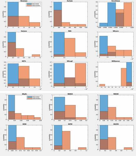
Figure 3 shows the frequency distribution of the 15 extracted multimodal features to distinguish the indoor PM from outdoor PM. Hussain et al. (2020a) extracted multimodal features and applied few supervised machine learning algorithms without feature selection methods and optimization using a similar data set and obtained a highest accuracy of 95.8% with a cubic and coarse Gaussian SVM and AUC of 1.00. In this study, we optimized parameters of 12 supervised machine learning algorithms. The detection performance was increased to 100% using SVM-L, SVM-R, RF, and XGB-T with original features. While using the chi-square feature selection method, the highest detection performance with an accuracy of 100% and an AUC of 1.00 was yielded using SVM-R, RF, XGB-T, and GBM.

Figure 3. Frequency distribution of various multimodal extracted features to distinguish the indoor particulate matter (PM) from outdoor PM.

Discussions

All pollutant exposures are increased and adverse effects are exacerbated by increased exposure concentration and/or longer exposure duration. The exposure being short or long term is categorized depending upon the duration contract with the pollutant. We can develop a correlation between the health effects including increased mortality and enduring exposure of the particulate matters. Long-term increased air pollution exposure can cause increased mortality by causing the cardiopulmonary disease and lung cancer (Cao et al., 2011). The severe health problems are caused due to the short-term exposure caused by the higher air pollutant concentration. The researchers in the past established correlation between interim exposure and ischemic heart diseases, asthma to air pollution, and unrelieved bronchitis (Pöschl, 2005). Moreover, a link is established between the exposure and increased mortality due to the short-term changes in particulate matters and daily deaths counts. The increased rate of hospitalization is also linked with the exposure of particulate matters. There is a great impact on the human health because of the size of the particulate matter (Brook et al., 2010). The small particles with a diameter of 10 μm can be bypassed within the nasal passage, thereby preventing the unwanted material to deposit in lungs and enter the body. The deposited particles are conceded through the alveolar lung’s membrane to the blood stream. The particulate matter, i.e. PM2.5, is associated with the increase of arrhythmia, stroke, heart, and heart failure (Brook et al., 2010). Moreover, gaseous copollutants and ultrafine particles are also implicated on the body due to the effects of particulate matter. The aerosol chemical composition reflects the origin of emissions. During the storm, the emitted particles have chemical compositions of dust, sulfate, nitrate, and organic and elemental carbon, and other responsible resources such as metal smelter can be correlated due to the increased threat of cardiac events (Ito et al., 2011). The increased health problems are also linked with the traffic sources. The mortality of cardiovascular diseases is also associated due to the combustion emission. The effect of these particles is still unclear that whether they are impaired or persuaded by small particles and diesel exhaust particles of components of the traffic mixture (Brook et al., 2010). In Brisbane, the particulate matters effects on pregnancy and birth defects were examined during health studies (L. Chen, Mengersen, & Tong, 2007; Hansen, Neller, Williams, & Simpson, 2007), hospital admissions, the air pollution, and interim and durable exposure effects on the cardio-respiratory system due to the particulate matter (Simpson et al., 2005). The prevalence of preterm birth and fatal growth reduction are still not examined with significant evidence along with the increased hospital admissions during bushfires and heavy traffic areas (Simpson et al., 2005).

The PM toxicity was computed by Ito et al. (2011) based on specific constituents, and bivariate chronological associations are determined between air pollution, weather, and outcomes of health variables by calculating the cross-correlation function (CCF) for the key variables. The temporal fluctuations can be determined using these cross-correlations. Previous studies (Ito et al., 2011; Rinehart et al., 2006) indicate that the relationship between two series is influenced powerfully by shared trends, day of week patterns, and seasonal cycles. The generalized linear regression models using the natural cubic spline smoothing function were used to compute the short-term variations. Moreover, Poisson generalization additive models (Schwartz, 1993; Stölzel et al., 2007) were employed to analyze the dynamics of particulate matters in different sizes and the daily mortality. Similarly, the locally weighted linear smooth function (Ruggeri et al. 2015) with a span of 0.05 was applied to control the trends and seasonal variations. The risk for each source including absolute factor scores was evaluated simultaneously in the model. The risk factor was evaluated by computing absolute factor scores simultaneously in the model. The city specific models were built to investigate which element is important for ambient particle toxicity (He, Mazumdar, & Arena, 2006; Laden et al. 2014; Urmila P. Kodavanti, Richard H. Jas, 1997) that includes daily measurement of lead, iron, sulfur, vanadium, manganese, nickel, and zinc as individual and in combination as well. The seasons, trends, and weather are also controlled for these factors.

The research from epidemiology indicates that both short- and long-term exposure of ambient indoor and outdoor particulate matters (PM) are associated with chronic and ambient hazardous health effects including cardiovascular and respiratory problems, lungs dysfunction, asthma attacks, etc. The PM data were acquired from different locations of Muzaffarabad Azad Kashmir for both indoor and outdoor PMs. Based on the dynamical characteristics of the PM time series, we extracted multifeatures such as frequency domain features and time-domain features, wavelet features, complexity-based entropy features, and statistical features from these particulate matters. The robust machine learning classifiers like SVM with cubic, quadratic, linear, and coarse gaussian were applied.

Hussain et al. utilized the same dataset (Hussain et al. 2020b), computed the multimodal features, and obtained the highest accuracy of 95.8% using SVM cubic and coarse Gaussian kernels and cubic KNN. We utilized primary data of indoor and outdoor collected from different locations of Muzaffarabad region of Azad Kashmir, Pakistan. Previously, researchers Saeed et al. (2017) and Shah et al. (2021) studied the nonlinear dynamical measures on this data set to unfold the nonlinear dynamics; however, this study is specifically aimed to develop an Artificial intelligence-based model based on multimodal features to capture the nonlinear dynamics and temporal and spectral changes of particulate matters time series from indoor and outdoor and provide a prediction with improved performance. In the recent study, we extracted the multimodal features by considering diverse factors to capture the multiple dynamics, optimized the machine learning algorithms, and applied the feature selection methods, which improved the particulate matter detection performance. In the recent study, most of the algorithms with optimization of parameters and applying the chi-square feature selection method yielded the highest improved performance and including SVM linear, SVM RBF, random forest, GBM, and XGB tree yielded the 100% sensitivity, specificity, PPV, NPV, and AUC followed by XGB linear with an accuracy of 97.92% and an AUC of 0.996. Moreover, without using the selection method, the highest performance was yielded using SVM RBF, RF, and GBM with 100% sensitivity, specificity, PPV, NPV, and AUC. Few algorithms also improved the performance based on the chi-square feature selection method such as SVM linear and XGB tree, which improved the accuracy from 93.75% to 100%.

The pollutant particulate matters affect adversely according to the size of particles, whereas the particulate matters having a size of approximately 10-micron can enter the lung directly and can affect it very severely. The particulate pollutant matters affect plants, human health, and the entire climate very severely. The particulate pollutions exposure can irritate the throat, eyes, and nose. It also attacks the bronchi and causes lung cancer. The increase of fine pollutant globally caused asthma. Therefore, accumulation of these particulate matters also caused the buildup of plaque in the vascular and arteries inflammation, which led to hardening of arteries and turn the heart problems. The pregnant mother can be affected along with the children because of the particulate matters during defects and failed pregnancy. The high level of aerosols and another pollutant can cause premature deaths. Globally, both the people of urban and rural areas are affected due to the PM exposure. However, in the rural areas, there are still old age cultivation systems and people are not taking the precautionary measures in working their daily life due to lack of awareness.

Conclusions

Due to the health-related risk associated with this inhalation of these particulates, the Particulates Matter has become a major concern in urban areas. PM comes from different sources, both organic and anthropogenic, of various aerodynamic dimensions, form, and solubility and chemical compositions (Seinfeld, Pandis, and Noone 1998). In the past two decades, extensive research on PM has resulted in some 1500–2,000 research papers per annum, thanks to advances in measuring technology and new methods and tools for dealing with public health problems. The findings show that these powerful classification methods are extremely useful for detecting and classifying indoor and outdoor tiny particles, which will aid in the development of automation systems for environmental improvement. Moreover, to unfold the concentration and severity levels, their associations with the diverse health affects require a proper data acquisition of PM from proposed working environments. This will help us to devise mechanisms and policies for people working in different working environments to reduce the mortality rates. Likewise, the nitrogen oxide and sulfur oxide affected from PM can severely affect our respiratory systems and lungs functionality, causing irritation of the eyes. Thus, the respiratory tract inflammation causes mucus secretion, coughing, aggravation of asthma, and chronic bronchitis and makes people more prone to infections of the respiratory tract. The proposed method provides an automated tool to accurately predict the particulate matter concentration, and concerned environmental and healthcare professionals can suggest an appropriate mechanism to minimize the severe effects produced by particulate matter concentration time series.

Availability of data and materials

The data set on Particulate Matter (PM2.5) concentrations was collected from the main campus of University of Azad Jammu and Kashmir, which is located at the roadside, leading from Combined Military Hospital (CMH) to upper Addah, of Muzaffarabad as detailed in Hussain et al. (2020a). The data can be provided on request.

Acknowledgments

The authors extend their appreciation to the Deanship of Scientific Research at King Khalid University for funding this work under grant number (RGP 2/46/43).

Princess Nourah bint Abdulrahman University Researchers supported Project number (PNURSP2022R114), Princess Nourah bint Abdulrahman University, Riyadh, Saudi Arabia.

The authors would like to thank the ‎Deanship of Scientific Research at Umm Al-Qura University ‎for supporting this work by Grant Code: (22UQU4310373DSR22).

Disclosure Statement

No potential conflict of interest was reported by the author(s).

References

- Albalak, R., G. J. Keeler, A. Roberto Frisancho, and M. Haber. 1999. Assessment of PM10 concentrations from domestic biomass fuel combustion in Two Rural Bolivian Highland Villages. Environmental Science and Technology 33 (15):402–432. doi:10.1021/es981242q.
- Ancelet, T., P. K. Davy, W. J. Trompetter, A. Markwitz, and D. C. Weatherburn. 2013. Carbonaceous aerosols in a wood burning community in rural New Zealand. Atmospheric Pollution Research 4 (3):245–49. doi:10.5094/APR.2013.026.
- Annesi-Maesano, I., F. Forastiere, N. Kunzli, and B. Brunekref. 2007. Particulate matter, science and EU policy. European Respiratory Journal 29 (3):428–31. doi:10.1183/09031936.00129506.
- Ariza-Lopez, F. J., J. Rodriguez-Avi, and M. V. Alba-Fernandez. 2018. Complete Control of an Observed Confusion Matrix. In IGARSS 2018-2018 IEEE International Geoscience and Remote Sensing Symposium, 2018-July:1222–25. IEEE, Valencia, Spain. 10.1109/IGARSS.2018.8517540.
- Avci, E., D. Hanbay, and A. Varol. 2007. An expert discrete wavelet adaptive network based fuzzy inference system for digital modulation recognition. Expert Systems with Applications 33 (3):582–89. doi:10.1016/j.eswa.2006.06.001.
- Bermejo, P., J. A. Gámez, and J. M. Puerta. 2014. Speeding up incremental wrapper feature subset selection with naive bayes classifier. Knowledge-Based Systems 55 (January):140–47. doi:10.1016/j.knosys.2013.10.016.
- Bradley, A. P. 1997. The use of the area under the ROC curve in the evaluation of machine learning algorithms. Pattern Recognition 30 (7):1145–59. doi:10.1016/S0031-3203(96)00142-2.
- Breiman, L. 1996. Bagging Predictors. Machine Learning 24 (2):123–40. doi:10.1007/BF00058655.
- Brook, R. K., S. J. Kutz, C. Millins, A. M. Veitch, B. T. Elkin, and T. Leighton. 2010. Evaluation and delivery of domestic animal health services in remote communities in the Northwest Territories: A case study of status and needs. The Canadian Veterinary Journal 51 (10):1115.
- Cai, L.-J., L. Shu, and K.-B. Shi. May 2021. Application of an improved CHI feature selection algorithm. Discrete dynamics in nature and society, , vol. 2021, 8. Article ID 9963382. doi:10.1155/2021/9963382.
- Cao, J., C. Yang, J. Li, R. Chen, B. Chen, D. Gu, and H. Kan. 2011. Association between long-term exposure to outdoor air pollution and mortality in China: A cohort study. Journal of Hazardous Materials 186 (2–3):1594–600.
- Chen, T., and C. Guestrin. 2016. XGBoost. In Proceedings of the 22nd ACM SIGKDD International Conference on Knowledge Discovery and Data Mining, 785–94. New York, NY, USA, New York, USA: ACM. 10.1145/2939672.2939785.
- Chen, L., K. Mengersen, and S. Tong. 2007. Spatiotemporal relationship between particle air pollution and respiratory emergency hospital admissions in Brisbane, Australia. The Science of the Total Environment 373 (1):57–67.
- Chen, Y. S., P. C. Sheen, E. R. Chen, Y. K. Liu, T. N. Wu, and C. Y. Yang. 2004. Effects of asian dust storm events on daily mortality in Taipei, Taiwan. Environmental Research 95 (2):151–55. doi:10.1016/j.envres.2003.08.008.
- Chen, C., G. Zhang, J. Yang, J. C. Milton, and A. D. Alcántara. 2016. An explanatory analysis of driver injury severity in rear-end crashes using a decision table/naïve bayes (DTNB) hybrid classifier. Accident Analysis & Prevention 90 (May):95–107. doi:10.1016/j.aap.2016.02.002.
- Costa, A. 2002. Determination of mechanical properties of traditional masonry walls in dwellings of Faial Island, Azores. Earthquake Engineering & Structural Dynamics 31 (7):1361–82. doi:10.1002/eqe.167.
- Criminisi, A. 2011. Decision forests: A unified framework for classification, regression, density estimation, manifold learning and semi-supervised learning. Foundations and Trends® in Computer Graphics and Vision 7 (2–3):81–227. doi:10.1561/0600000035.
- Dheeba, J., N. Albert Singh, and S. Tamil Selvi. 2014. Computer-aided detection of breast cancer on mammograms: A swarm intelligence optimized wavelet neural network approach. Journal of Biomedical Informatics 49:45–52. doi:10.1016/j.jbi.2014.01.010.
- Dobrowolski, A. P., M. Wierzbowski, and K. Tomczykiewicz. 2012. Multiresolution MUAPs decomposition and SVM-Based analysis in the classification of neuromuscular disorders. Computer Methods and Programs in Biomedicine 107 (3):393–403. doi:10.1016/j.cmpb.2010.12.006.
- Fang, X., H.-F. Guo, S. Husodo, B. C. Paasch, T. M. Bridges, D. Santelia, O. Kötting, C. W. Vander Kooi, and M. S. Gentry. 2013. ve Bayes: Inference-Based Naı ¨ ve Bayes Cost-Sensitive Turning Naı. The Plant Cell 25 (10):2302–14. doi:10.1109/TKDE.2012.196.
- Ferland, R. J., J. Smith, D. Papandrea, J. Gracias, L. Hains, S. B. Kadiyala, B. O’Brien, E. Y. Kang, B. S. Beyer, and B. J. Herron. 2017. Multidimensional genetic analysis of repeated seizures in the hybrid mouse diversity panel reveals a novel epileptogenesis susceptibility locus. G3 (Bethesda, Md.) g3.117.042234. doi:10.1534/g3.117.042234.
- Friedman, J. H. 2001. Greedy function approximation: A gradient boosting machine. Annals of Statistics 29 (5):1189–232. doi:10.2307/2699986.
- Friedman, J. H. 2002. Stochastic Gradient Boosting. Computational Statistics & Data Analysis 38 (4):367–78. doi:10.1016/S0167-9473(01)00065-2.
- Gammerman, A., Z. Luo, J. Vega, and V. Vovk. 2016. Conformal and probabilistic prediction with applications: 5th international symposium, COPA 2016 madrid, Spain, April 20- 22,2016 Proceedings. Lecture Notes in Computer Science (Including Subseries Lecture Notes in Artificial Intelligence and Lecture Notes in Bioinformatics) 9653:185–95. doi:10.1007/978-3-319-33395-3.
- Gao, C.-Z., Q. Cheng, H. Pei, W. Susilo, and L. Jin. 2018. Privacy-Preserving naive bayes classifiers secure against the substitution-then-comparison attack. Information Sciences 444 (1):72–88. doi:10.1016/j.ins.2018.02.058.
- Genuer, R., J.-M. Poggi, and C. Tuleau-Malot. 2010. Variable selection using random forests. Pattern Recognition Letters 31 (14):2225–36. doi:10.1016/j.patrec.2010.03.014.
- Glasius, M., M. Ketzel, P. Wahlin, B. Jensen, J. Monster, R. Berkowicz, and F. Palmgren. 2006. Impact of wood combustion on particle levels in a residential area in denmark. Atmospheric Environment 40 (37):7115–24. doi:10.1016/j.atmosenv.2006.06.047.
- Grange, S. K., J. A. Salmond, W. J. Trompetter, P. K. Davy, and T. Ancelet. 2013. Effect of atmospheric stability on the impact of domestic wood combustion to air quality of a small urban township in winter. Atmospheric Environment 70 (May):28–38. doi:10.1016/j.atmosenv.2012.12.047.
- Hansen, C., A. Neller, G. Williams, and R. Simpson. 2007. Low levels of ambient air pollution during pregnancy and fetal growth among term neonates in Brisbane, Australia. Environmental Research 103 (3):383–89.
- He, S., S. Mazumdar, and V. C. Arena. 2006. A comparative study of the use of GAM and GLM in air pollution research. Environmetrics: The Official Journal of the International Environmetrics Society 17 (1):81–93.
- Hussain, L., W. Aziz, Z. H. Kazmi, and I. A. Awan. 2014. Classification of human faces and non faces using machine learning techniques. International Journal of Electronics and Electrical Engineering 2 (2):116–23. doi:10.12720/ijeee.2.2.116-123.
- Hussain, L., W. Aziz, S. Saeed, M. Rafique, M. S. A. Nadeem, S.-O. Shim, S. Aftar, and J.-U.-R. Pirzada. 2020a. Extracting mass concentration time series features for classification of indoor and outdoor atmospheric particulates. Acta Geophysica 68 (3):945–63. doi:10.1007/s11600-020-00443-y.
- Hussain, L., W. Aziz, S. Saeed, M. Rafique, M. S. A. Nadeem, S.-O. Shim, S. Aftar, and J.-U.-R. Pirzada. 2020b. Extracting mass concentration time series features for classification of indoor and outdoor atmospheric particulates. Acta Geophysica 68 (3):945–63. doi:10.1007/s11600-020-00443-y.
- Hussain, L., W. Aziz, S. Saeed, S. A. Shah, M. S. A. Nadeem, I. A. Awan, A. Abbas, A. Majid, and S. Z. H. Kazmi. 2017a. Quantifying the Dynamics of Electroencephalographic (EEG) signals to distinguish alcoholic and non-alcoholic subjects using an MSE Based K-d tree algorithm. Biomedical Engineering/Biomedizinische Technik doi:10.1515/bmt-2017-0041.
- Hussain, L., I. Shafi, S. Saeed, A. Abbas, I. A. Awan, S. A. Nadeem, S. Z. H. Kazmi, and S. A. Shah. 2017b. A radial base neural network approach for emotion recognition in human speech. International Journal of Computer Science and Network Security 17 (8):52–62.
- Ito, K., R. Mathes, Z. Ross, A. Nádas, G. Thurston, and T. Matte. 2011. Fine particulate matter constituents associated with cardiovascular hospitalizations and mortality in New York City. Environmental Health Perspectives 119 (4):467–73.
- Jin, X., X. Anbang, R. Bie, and P. Guo. 2006. Machine learning techniques and chi-square feature selection for cancer classification using SAGE gene expression profiles. In International workshop on data mining for biomedical applications (pp. 106-115). Springer, Berlin, Heidelberg. doi:10.1007/11691730_11.
- Kodavanti, U. P., R. H. Jaskot, W. Y. Su, D. L. Costa, A. J. Ghio, and K. L. Dreher. 1997. Genetic variability in combustion particle-induced chronic lung injury. American Journal of Physiology-Lung Cellular and Molecular Physiology 272 (3):L521–L532.
- Kohavi, R., and G. H. John. 1997. Wrappers for feature subset selection. Artificial Intelligence 97 (1–2):273–324. doi:10.1016/S0004-3702(97)00043-X.
- Laden, F., L. M. Neas, D. W. Dockery, J. Schwartz, and Y. Li. 2014. “Association of fine particulate matter from different sources with daily mortality in six association of fine particulate matter from different sources with Daily Mortality in Six U. S. Cities. Respiratory Medicine 108 (10):941–47. doi:10.1289/ehp.00108941.
- Lipsett, M., S. Hurley, and B. Ostro. 1997. Air pollution and emergency room visits for asthma in santa clara county, california. Environmental Health Perspectives 105 (2):216–22. doi:10.1289/ehp.97105216.
- Lu, Y., Y. Ma, C. Chen, and Y. Wang. 2018. Classification of single-channel EEG signals for epileptic seizures detection based on hybrid features. Technology and Health Care 26 (S1):337–46.
- Mar, T. F., K. Ito, J. Q. Koenig, T. V. Larson, D. J. Eatough, R. C. Henry, E. Kim, F. Laden, R. Lall, L. Neas, et al. 2006. PM source apportionment and health effects. 3. investigation of inter-method variations in associations between estimated source contributions of PM2.5 and daily mortality in phoenix, AZ. Journal of Exposure Science and Environmental Epidemiology 16 (4):311–20. doi:10.1038/sj.jea.7500465.
- McGowan, J. A., P. N. Hider, E. Chacko, and G. I. Town. 2002. Particulate air pollution and hospital admissions in christchurch, New Zealand. Australian and New Zealand Journal of Public Health 26 (1):23–29. doi:10.1111/j.1467-842X.2002.tb00266.x.
- Molnár, P., and G. Sallsten. 2013. Contribution to PM2.5 from domestic wood burning in a small community in sweden. Environmental Science: Processes & Impacts 15 (4):833. doi:10.1039/c3em30864b.
- Naeher, L. P., M. Brauer, M. Lipsett, J. T. Zelikoff, C. D. Simpson, J. Q. Koenig, and K. R. Smith. 2007. Woodsmoke health effects: A review. Inhalation Toxicology 19 (1):67–106. doi:10.1080/08958370600985875.
- Naeher, L. P., K. R. Smith, B. P. Leaderer, L. Neufeld, and D. T. Mage. 2001. Carbon monoxide as a tracer for assessing exposures to particulate matter in wood and gas Cookstove Households of Highland Guatemala. Environmental Science and Technology 35 (3):575–81. doi:10.1021/es991225g.
- Ostro, B. D., R. Broadwin, and M. J. Lipsett. 2000. Coarse and fine particles and daily mortality in the coachella valley, california: A follow-up study. Journal of Exposure Analysis and Environmental Epidemiology 10 (5):412–19. doi:10.1038/sj.jea.7500094.
- Pan, Y. H., W. Y. Lin, Y. H. Wang, and K. T. Lee. 2011. Computing multiscale entropy with orthogonal range search. Journal of Marine Science and Technology 19 (1):107–13. doi:10.51400/2709-6998.2143.
- Portnov, B. A., and S. A. Paz. 2008. Climate Change and Urbanization in Arid Regions. Annals of Arid Zone 47 (3 & 4):1–15.
- Portnov, B. A., S. Paz, and L. Shai. 2011. What does the inflow of patients into the rambam medical center in haifa tells us about outdoor temperatures and air pollution? Geography Research Forum 31:39–52.
- Pöschl, U. 2005. Atmospheric aerosols: Composition, transformation, climate and health effects. Angewandte Chemie International Edition 44 (46):7520–40.
- Rathore, S., M. Hussain, M. A. Iftikhar, and A. Jalil. 2014. Ensemble classification of colon biopsy images based on information rich hybrid features. Computers in Biology and Medicine 47 (1):76–92. doi:10.1016/j.compbiomed.2013.12.010.
- Rathore, S., M. Hussain, and A. Khan. 2015. Automated colon cancer detection using hybrid of novel geometric features and some traditional features. Computers in Biology and Medicine 65 (October):279–96. doi:10.1016/j.compbiomed.2015.03.004.
- Reinhardt, J. P., K. Boerner, and A. Horowitz. 2006. Good to have but not to use: Differential impact of perceived and received support on well-being. Journal of Social and Personal Relationships 23 (1):117–29.
- Rosidin, S., G. F. Shidik, A. Z. Fanani, and F. Al Zami, and Purwanto. 2021. Improvement with chi square selection feature using supervised machine learning approach on covid-19 data. In 2021 International Seminar on Application for Technology of Information and Communication (ISemantic), 32–36. IEEE, Semarangin, Indonesia. 10.1109/iSemantic52711.2021.9573196.
- Rosso, O. A., S. Blanco, J. Yordanova, V. Kolev, A. Figliola, M. Schürmann, and E. Başar. 2001. Wavelet Entropy: A new tool for analysis of short duration brain electrical signals. Journal of Neuroscience Methods 105 (1):65–75. doi:10.1016/S0165-0270(00)00356-3.
- Rostami, M., K. Berahmand, and S. Forouzandeh. 2021. A novel community detection based genetic algorithm for feature selection. Journal of Big Data 8 (1):2. doi:10.1186/s40537-020-00398-3.
- Rostami, M., S. Forouzandeh, K. Berahmand, M. Soltani, M. Shahsavari, and M. Oussalah. 2022. Gene selection for microarray data classification via multi-objective graph theoretic-based method. Artificial Intelligence in Medicine 123 (January):102228. doi:10.1016/j.artmed.2021.102228.
- Ruggeri, J., A. V. Longo, M. P. Gaiarsa, L. R. Alencar, C. Lambertini, D. S. Leite, and M. Martins. 2015. Seasonal variation in population abundance and chytrid infection in stream-dwelling frogs of the Brazilian Atlantic forest. PloS One 10 (7):e0130554.
- Saberi-Movahed, F., M. Mohammadifard, A. Mehrpooya, M. Rezaei-Ravari, K. Berahmand, M. Rostami, S. Karami, M. Najafzadeh, D. Hajinezhad, M. Jamshidi, et al. 2021. July. Decoding Clinical Biomarker Space of COVID-19: Exploring Matrix Factorization-based Feature Selection Methods. MedRxiv: The Preprint Server for Health Sciences. 10.1101/2021.07.07.21259699.
- Saeed, S., W. Aziz, M. Rafique, I. Ahmad, K. J. Kearfott, and S. Batoolb. 2017. Quantification of non-linear dynamics and chaos of ambient particulate matter concentrations in muzaffarabad city. Aerosol and Air Quality Research 17 (3):849–56. doi:10.4209/aaqr.2016.04.0137.
- Saeys, Y., I. Inza, and P. Larranaga. 2007. A review of feature selection techniques in bioinformatics. Bioinformatics 23 (19):2507–17. doi:10.1093/bioinformatics/btm344.
- Sarnat, J. A., A. Marmur, M. Klein, E. Kim, A. G. Russell, S. E. Sarnat, J. A. Mulholland, P. K. Hopke, and P. E. Tolbert. 2008. Fine particle sources and cardiorespiratory morbidity: An application of chemical mass balance and factor analytical source-apportionment methods. Environmental Health Perspectives 116 (4):459–66. doi:10.1289/ehp.10873.
- Schlesinger, R. B., N. Kunzli, G. M. Hidy, T. Gotschi, and M. Jerrett. 2006. The health relevance of ambient particulate matter characteristics: Coherence of toxicological and epidemiological inferences. Inhalation Toxicology 18 (2):95–125. doi:10.1080/08958370500306016.
- Schwartz, J. 1993. Air pollution and daily mortality in Birmingham, Alabama. American Journal of Epidemiology 137 (10):1136–47.
- Seinfeld, J. H., S. N. Pandis, and K. Noone. 1998. Atmospheric chemistry and physics: From air pollution to climate change. Physics Today 51 (10):88. doi:10.1063/1.882420.
- Shah, S., A. Ali, W. Aziz, M. Almaraashi, M. S. A. Nadeem, H. Nazneen, and S.-O. Shim. 2021. A hybrid model for forecasting of particulate matter concentrations based on multiscale characterization and machine learning techniques. Mathematical Biosciences and Engineering 18 (3):1992–2009. doi:10.3934/mbe.2021104.
- Shrestha, U., A. Alsadoon, P. W. C. Prasad, S. Al Aloussi, and O. H. Alsadoon. 2021. Supervised machine learning for early predicting the sepsis patient: modified mean imputation and modified chi-square feature selection. Multimedia Tools and Applications 80 (13):20477–500. doi:10.1007/s11042-021-10725-2.
- Simpson, F., S. Martin, T. M. Evans, M. Kerr, D. E. James, R. G. Parton, and C. Wicking. 2005. A novel hook‐related protein family and the characterization of hook‐related protein 1. Traffic 6 (6):442–58.
- Stölzel, M., S. Breitner, J. Cyrys, M. Pitz, G. Wölke, W. Kreyling, and A. Peters. 2007. Daily mortality and particulate matter in different size classes in Erfurt, Germany. Journal of Exposure Science & Environmental Epidemiology 17 (5):458–67.
- Subasi, A. 2013. Classification of EMG signals using PSO optimized SVM for diagnosis of neuromuscular disorders. Computers in Biology and Medicine 43 (5):576–86. doi:10.1016/j.compbiomed.2013.01.020.
- Town, G. I. 2001. The health effects of particulate air pollution - a christchurch perspective. Biomarkers 6 (1):15–18. doi:10.1080/135475001452742.
- Trompetter, W. J., S. K. Grange, P. K. Davy, and T. Ancelet. 2013. Vertical and temporal variations of black carbon in new zealand urban areas during winter. Atmospheric Environment 75 (August):179–87. doi:10.1016/j.atmosenv.2013.04.036.
- Vapnik, V. N. 1999. An overview of statistical learning theory. IEEE Transactions on Neural Networks/a Publication of the IEEE Neural Networks Council 10 (5):988–99. doi:10.1109/72.788640.
- Wang, H., T. M. Khoshgoftaar, and K. Gao. 2010. A comparative study of filter-based feature ranking techniques. In 2010 IEEE International Conference on Information Reuse & Integration, 1. 43–48. IEEE, Las Vegas, NV, USA. 10.1109/IRI.2010.5558966.
- Wang, D., D. Miao, and C. Xie. 2011. Best basis-based wavelet packet entropy feature extraction and hierarchical EEG classification for epileptic detection. Expert Systems with Applications 38 (11):14314–20. doi:10.1016/j.eswa.2011.05.096.
- Wang, L.-M., L. Xiao-Lin, C.-H. Cao, and S.-M. Yuan. 2006. Combining decision tree and naive bayes for classification. Knowledge-Based Systems 19 (7):511–15. doi:10.1016/j.knosys.2005.10.013.
- Wang, L., W. Xue, L. Yang, M. Luo, J. Huang, W. Cui, and C. Huang. 2017. Automatic epileptic seizure detection in EEG signals using multi-domain feature extraction and nonlinear analysis. Entropy 19 (6):222. doi:10.3390/e19060222.
- Weng, Y.-C., N.-B. Chang, and T. Y. Lee. 2008. Nonlinear time series analysis of ground-level ozone dynamics in southern taiwan. Journal of Environmental Management 87 (3):405–14. doi:10.1016/j.jenvman.2007.01.023.
- Wu, Y., Y. Zhou, G. Saveriades, S. Agaian, J. P. Noonan, and P. Natarajan. 2013. Local shannon entropy measure with statistical tests for image randomness. Information Sciences 222 (February):323–42. doi:10.1016/j.ins.2012.07.049.
- Yamauchi, Y., and M. Mukaidono. 1999. Probabilistic inference and bayesian theorem based on logical implication. In Lecture Notes in Computer Science, 334–42. Berlin, Heidelberg: Springer. doi:10.1007/978-3-540-48061-7_40.
- Yu, L., and H. Liu. 2003. Efficiently handling feature redundancy in high-dimensional data. In Proceedings of the Ninth ACM SIGKDD International Conference on Knowledge Discovery and Data Mining - KDD ’03, 685, Washington, DC, USA. ACM Press. 10.1145/956750.956840.
- Yuan, G.-X., H. Chia-Hua, and C.-J. Lin. 2012. Recent advances of large-scale linear classification. Proceedings of the IEEE 100 (9):2584–603. doi:10.1109/JPROC.2012.2188013.
- Zaidi, N. A., Y. Du, and G. I. Webb. 2020. On the effectiveness of discretizing quantitative attributes in linear classifiers. IEEE Access 8:198856–71. doi:10.1109/ACCESS.2020.3034955.
- Zhang, J., C. Chen, Y. Xiang, W. Zhou, and Y. Xiang. 2013. Internet Traf Fi c classi fi cation by aggregating correlated naive bayes predictions. IEEE Trans. Information Forensics and Security 8 (1):5–15. doi:10.1109/TIFS.2012.2223675.
- Zhao, Z., and H. Liu. 2007. Spectral feature selection for supervised and unsupervised learning. In Proceedings of the 24th International Conference on Machine Learning - ICML ’07, 1151–57. New York, New York, USA: ACM Press. 10.1145/1273496.1273641.