A Novel Augmentative Backward Reward Function with Deep Reinforcement Learning for Autonomous UAV Navigation

ABSTRACT

The autonomous UAV (unmanned aerial vehicle) navigation has recently gained an increasing interest from both academic and industrial sectors due to its potential uses in various fields and especially, the need for social distancing during the pandemic. Many works have adopted a deep reinforcement learning (RL) method with experience replay called deep deterministic policy gradient (DDPG) to control the motion of UAV, and gain high accuracy results in static and simplified environments. However, they are still far from being ready for real world adoption in that the UAVs have to operate under complex and dynamic conditions. We also found that using only DDPG makes the learning process prone to oscillation and is inefficient for tasks having high dimensional action-state spaces. Furthermore, the goal reward mechanism in traditional reward functions brings a bias to the state, which resembles the one at the goal area and leads to erroneous action selection. To get closer to being ready for real world adoption, we proposed a novel method that enables UAVs to be capable of handling motion control in realistic environments. The first component of our proposed method is point cloud data (PCD) simplification with truncated icosahedron structure which converts enormous PCD into a few essential data points. In the second component of our method, we replace the traditional goal reward mechanism with a new mechanism called Augmentative Backward Reward (ABR) function to dispense the goal reward to transitions proportionately to its participation. By integrating simplified PCD and ABR, we achieved significantly better results when compared with using only the-state-of-the-art, TD3. In addition, we tested the proposed method with another navigation task, BipedalWalkerHardcore, a testbed for RL, and the result is still better and steadier than of TD3. These results indicate that the proposed method is robust.

KEYWORDS:

• UAV
• deep reinforcement learning
• navigation
• reward function
• point cloud data

Introduction

With the flourishing of deep learning, numerous smart applications, innovative devices and vehicles have been introduced in abundance (Falanga, Kleber, and Scaramuzza 2020). Furthermore, with the current pandemic in many countries, people nowadays need more modern solutions that are safer. The unmanned aerial vehicle (UAV) is one of those solutions to mitigate man’s burden. There are many hindrances in developing autonomous UAV, such as the expensive cost of UAV and its sensor, enormous size of receiving data, multidimensional movement, and catastrophic damage in the event of crash (MAHMUD 2021)

Many researchers have operated on autonomous UAV navigation and implemented many techniques to reach a step closer to real world adoption. Traditional methods often used to navigate are path-motion planning algorithms like Rapid Random Tree (RRT) (Youn et al. 2020), A* (Erke et al. 2020), Grid-Graph based (Hajdu and Ballagi 2020) and Reinforcement Learning (RL) (Zijian et al. 2020). These methods can achieve sufficiently high accuracy results but with limitations that prior knowledge or certain information of the environment is required – that is, only discrete interaction with the environment is allowed and state-action spaces are finite, which in fact, in the real-world environment, all of these are often unknown and controversial. Hence, there are efforts to overcome these limitations (Tan, Yan, and Guan 2017). One of the most successful methods in the limelight is, advanced Deep Reinforcement Learning (DRL), the deep deterministic policy gradient (DDPG) (Lillicrap et al. 2015). It can achieve quite good results even in continuous space problems.

Having said that, much research still indicates that only DDPG is insufficient for dynamics and complex environments. Some of them mentioned that it is irrational to assume all transitions are equal since it is ignoring the fact that there are differences in the value of each individual transition, thus more rational sampling strategy should be applied to replace uniform random strategy. Hou and Zhang (2019) applied prioritized experience replay (PER) technique which prioritizes the importance as TD Error of each transition to DDPG and the result shows that prioritizing the experience replay could make the network more stable. Additionally, Fujimoto, van, and Meger (2018) also pointed out to emphasize the same problem that the main concern of DDPG is its instability. DDPG is fragile regarding hyper-parameters and some kinds of tuning. A result heavily relies on correct setting of these for the certain tasks because the critic (Q-function) dramatically overestimates Q-value, and consequently, can lead to the agent falling into the local optima or perhaps catastrophic forgetting of experience. There are other works that tried to alleviate instability problems with different methods, such as with recurrent networks (Kapturowski et al. 2018) and some mechanisms (Zijian et al. 2020). Despite a number of techniques trying to accomplish the stability problem of DDPG, the clear path to real-world adoption is still obscure since it still also needs efficiency and complex environmental support.

Besides the control motion problem, in autonomous UAV navigation, the environmental perception is another problem. There are many kinds of equipment used to simulate vision of UAV such as RGB camera, depth camera, ranging sensor (RADAR), light detection and ranging sensor (LiDAR). The output of these equipment differs from one another, and are suitable for different tasks too. For navigation tasks, LiDAR is recently the most popular (Kolar, Benavidez, and Jamshidi 2020) due to its capability to accurately measure distance to the object by analyzing the reflected light regardless of whether it is day or night time, and also be able to generate half a million of 3D point-cloud data (PCD) per second. Moreover, to process thoroughly on huge data could be a heavy computational burden for the onboard computer of UAV. The data with that size could cause near infinite patterns of sight and be supernumerary for RL to learn.

Overall, the hindrances to real world adoption of UAV can be divided into two issues. First, current control motion algorithms (Zijian et al. 2020) achieve just a moderate success rate and only in simple environments, low state-action spaces. Second, an approach to deal with the huge size of PCD for navigation still does not exist. Therefore, we propose a comprehensive approach that makes autonomous UAV navigation reach real-world adoption more than ever. The main contributions of this work are as follows:

(1) Structuring of Realistic 3D Simulation for UAV Control Motion Problem

The environment, UAV and sensor used in this work were simulated in the same detail, size, and weight as reality by GAZEBO simulator (Koenig and Howard 2004). The LiDAR sensor is the same specification as the actual device. In addition, the physics system, gravity, aerodynamic, and magnetic field were set just as the same as the world’s. Changing the difficulty level can be done by changing the scenario of the environment such as a valley, forest, city, etc.

(2) Point Cloud Simplification with Truncated Icosahedron Structure

A structure that looks like a soccer ball (Truncated Icosahedron) is used to be a representative of PCD. With this structure, around three hundred thousand points turn into thirty-two sides joined to each other. This simulated ball covers and moves along the UAV. Each side of the ball warns the UAV whenever there is a point cloud found inside, that is, the UAV is touching something. This mechanism helps the UAV to pay attention only for what it needs to, so the number of patterns is affordable to learn.

(3) Sequential Transition Learning

For typical RL, the agent stores what it currently perceives to the buffer as a transition and this transition is merely one frame information. It is difficult to know the meaning of this laconic transition, for instance, if we take a photo of two humans playing table tennis and ask someone “In the photo, in what direction the ball will move next, up or down?.” Thus, it is better to adopt sequential transition, which is the sequence of observations ($o_1,o_2,\dots ,o_n$), especially for some types of path-planning tasks.

(4) Augmentative Backward Reward Function

Often used reward functions for control motion problems commonly have three conditions – if arrived, collided and other. Usually, when the agent collides with an obstacle, it should get a punishment in the form of negative or less reward to dissuade this behavior and, when it reaches the goal, it gets a big amount of reward to urge this behavior. The problem is that giving big rewards like this to just one transition is irrational and this makes the agent have bias to that transition. For instance, if the goal is located at the left bend, whenever the agent meets the left bend, it will be heavily urged to turn left even though that is not a good decision. Therefore, we proposed the novel and more rational reward function, ABR function, which has a mechanism that can provide the dynamic reward proportion to the usefulness of transition in a backward fashion. Sequential transition, simplified PCD and ABR not only make the DRL robust against various environments but also gain desirable results.

Background

In a standard autonomous navigation problem, there only exist two things physically, environment and agent. Although the objective is simple, which is to control the agent to the goal, making it efficient needs many components. This section will describe the detail of each component.

UAV Model

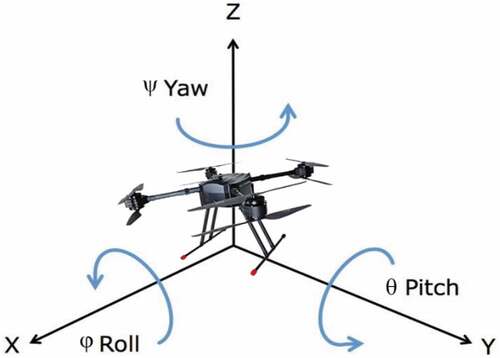
UAV is an aircraft without any human pilot. The kind of UAV used in this work was quadrotor due to its advantage over other kinds such that it can maneuver comfortably like capable of taking-off and landing vertically and can surprisingly lift the heavier payload compared to its own weight. As the name suggests, this UAV has four rotors located at the vertex of a square frame spinning to move six degrees of freedom (6DoF). This means that to control this UAV requires six variables $\left(l_x,l_y,l_z,a_x,a_y,a_z\right)$. The first three variables denote linear velocity along x, y, z axes, respectively. As shown in Figure 2.1, the other three variables denote angular velocity along x, y, z axes and the rotation along these axes were called roll pitch yaw angles ($\phi ,\theta ,\psi$), respectively.

Figure 2.1. UAV position and Euler angles in 3D simulation environment.

In a realistic environment such as the one used in this work, the forces and moments produced by rotors were dampened during the flight by external forces including gravity and aerodynamic forces, so, to find the changes of UAV’s motion can be done as follows:

(2.1) $C=\left[\begin{array}{c}{F}_{mx}\\ F_{my}\\ F_{mz}\\ M_{mx}\\ M_{my}\\ M_{mz}\end{array}\right]-(E_g+E_a)$(2.1)

(2.2) $\begin{array}{c}{F}_{mx}=m({\dot{l}}_x+a_y{l}_z-a_z{l}_y)-S_x(a_y^2+a_z^2)-S_y({\dot{a}}_z-a_x{a}_y)+S_z({\dot{a}}_y+a_x{a}_z)\\ F_{my}=m(l_y+a_z{l}_x-a_x{l}_z)+S_x({\dot{a}}_z+a_x{a}_y)-S_y(a_x^2+a_z^2)-S_z({\dot{a}}_x-a_y{a}_z)\\ F_{mz}=m({\dot{l}}_z+a_x{l}_y-a_y{l}_x)-S_x({\dot{a}}_y+a_x{a}_z)+S_y({\dot{a}}_x+a_y{a}_z)-S_z(a_y^2+a_x^2)\end{array}$(2.2)

$M_{mx}=I_x{\dot{a}}_x-(I_y-I_z)a_y{a}_z-I_{xy}({\dot{a}}_y-a_x{a}_z)-I_{xz}({\dot{a}}_z+a_x{a}_y)-I_{yz}(a_y^2-a_z^2)+S_y({\dot{l}}_z+a_x{l}_y-a_y{l}_x)+S_z(a_x{l}_z-a_z{l}_x-{\dot{l}}_y)$

$M_{my}=I_y{\dot{a}}_y-(I_z-I_x)a_z{a}_x-I_{xy}({\dot{a}}_x+a_y{a}_z)-I_{yz}({\dot{a}}_z-a_x{a}_y)-I_{xz}(a_z^2-a_x^2)-S_x({\dot{l}}_z+a_x{l}_y-a_y{l}_x)+S_z({\dot{l}}_x-a_z{l}_y+a_y{l}_z)$

$M_{mz}=I_z{\dot{a}}_z-\left(I_x-I_y\right)a_x{a}_y-I_{yz}\left({\dot{a}}_y+a_x{a}_z\right)-I_{xz}\left({\dot{a}}_x-a_z{a}_y\right)-I_{xy}\left(a_x^2-a_y^2\right)+S_x\left({\dot{l}}_y-a_x{l}_z+a_z{l}_x\right)-S_y\left({\dot{l}}_x-a_z{l}_y+a_y{l}_z\right)$

$C$ denotes vector of translational and rotational changes in UAV’s motion regarding to gravity force, $E_g$ and aerodynamics force, $E_a$ performed against UAV’s flight.

where $F$ = force, $M$ = moment, $m$ = the mass of UAV, $I_x,I_y,I_z$ = moments of inertia related to UAV axes, $I_{xy},I_{yz},I_{zx}$ = moments of UAV deviation, $S_x,S_y,S_z$= static moments related to UAV axes.

(2.3) $E_g=mg\left[\begin{array}{c}-sin\theta \\ cos\theta sin\phi \\ cos\theta cos\phi \\ 0\\ 0\\ 0\end{array}\right]$(2.3)

where $g$ = gravitational acceleration $(9.81/{\mathrm{s}}^2)$. (Since gravity acts through the center of gravity point of the UAV, it creates no moment.)

$E_a=\left[\begin{array}{c}{F}_a\\ M_a\end{array}\right]\alpha =\mathrm{a}\mathrm{r}\mathrm{c}\mathrm{t}\mathrm{a}\mathrm{n}\frac{l_z}{l_x}\beta =\mathrm{a}\mathrm{r}\mathrm{c}\mathrm{s}\mathrm{i}\mathrm{n}\frac{l_y}{l_{y0}}$

$TM=\left[\begin{array}{c}cos\alpha cos\beta cos\alpha sin\beta -sin\alpha \\ -sin\beta cos\beta 0\hspace{0.17em}\\ -sin\alpha cos\beta sin\alpha sin\beta cos\alpha \end{array}\right]A=\frac{1}{2}\rho S_f{l}_{y0}^2$

(2.4) $F_a=ATM\left[\begin{array}{c}{C}_x\\ C_y\\ C_z\end{array}\right]+\left[\begin{array}{c}{X}_y{a}_y\\ Y_x{a}_x+Y_z{a}_z\\ Z_y{a}_y\end{array}\right]$(2.4)

$M_a=A\left[\begin{array}{ccc}0& -z_a& y_a\\ z_a& 0& -x_a\\ -y_a& x_a& 0\end{array}\right]TM\left[\begin{array}{c}{C}_x\\ C_y\\ C_z\end{array}\right]+ATM\left[\begin{array}{c}{C}_l\\ C_m\\ C_n\end{array}\right]+\left[\begin{array}{c}{L}_x{a}_x+L_z{a}_z\\ M_y{a}_y\\ N_x{a}_x+N_z{a}_z\end{array}\right]$

where $\alpha ,\beta$ = UAV approach and slide angles respectively, $\rho \left(Alt\right)$ = air density at given altitude, $S_f$ = the surface of UAV, $x_a,y_a,z_a$ = distances between the aerodynamic center and UAV’s center of gravity, $C_x,C_y,C_z$ = coefficients of components of aerodynamic forces: resistance, side and carrier force, $C_l,C_m,C_n$ = coefficients of reclination, tilt and slumping aerodynamic moments, $X_y,Y_x,Y_z,Z_y,L_x,L_z,M_y,N_x,N_z$ = derivatives of components of the aerodynamic forces and moments respected to components of linear and angular velocities.

Reinforcement Learning

This work is based on the RL framework (Sutton and En A. G 1999), in which the agent interacts with the environment to maximize the total reward. The RL problem can be formulated as a Markov Decision Process (MDP) (Bellman 1957), it usually consists of five attributes ($S,A,P,R,\gamma$), where $S$ is set of states, $A$ set of action, $P$ probability of doing action $a$ at state $s$ to reach ${ }^1$. $R$ reward receiving after transiting from $s$ to $s$. $\gamma \in \left[0,1\right]$ discount factor which determines the agent’s preference to the reward achieved in the past, present, and future, if $\gamma =0$ the agent will be myopia and only learn on the actions that provide an intermediate reward. At each discrete time step $t$, the agent receives an observation $o_t$, which may be a part or whole of state $s_t$, and take action $a_t$ to environment with regarding to this state, after that the agent receives reward $r_t$ and is changed to a next state $s_{t+1}$. This action UAV take is determined by policy ${\mu }_{\theta }$ with parameters $\theta$. In discrete state-action spaces, finding optimal policy can usually be affordable, such as by greedily selecting maximum-reward action – however, in continuous spaces, it will be a totally different story.

Deep Reinforcement Learning is RL having an experience replay buffer which is used to overcome the strong temporal correlations caused by sequentially generated states in RL. The experience replay utilizes memory by storing past transitions and, in each iteration, the fixed sized transitions are randomly selected to update the network parameters. As a result, DRL achieves quite good results beyond human-level performance in certain tasks, Atari (Mnih et al. 2013) for example, and also has fewer limitations.

Deep Deterministic Policy Gradient (DDPG) for UAV Navigation

DDPG, as aforementioned, is the most promising method in the continuous domain. Lillicrap et al. (2015) broke the limitation of discrete action space in DQN (Deep Q Network) with DPG and proposed a state of art actor-critic framework. In DQN, the policy can be formulated as follow:

(2.5) $\mu \left(s\right)=argma{x}_{a}Q\left(s,a\right)$(2.5)

An optimal action is derived from taking argument max over the Q-values of all actions. DDPG bypasses this by directly outputting the action through the actor. For DDPG, the actor-critic framework consists of two eponymous networks and each network also has two sibling-like neural networks called eval-net and target-net. Actor which is used as a policy $\mu \left(s|{\theta }^{\mu }\right)$ map a state to action and critic $Q\left(s,a|{\theta }^Q\right)$ criticize how good the actor performs in the form of Q-value. To update the parameters, actor adopts DPG algorithm proved by Silver et al. (2014):

(2.6) ${\mathrm{\nabla }}_{{\theta }^{\mu }}J\left({\theta }^{\mu }\right)=\frac{1}{N}{\sum }_{i=1}^N{\mathrm{\nabla }}_{a}Q\left(s_i,a|{\theta }^Q\right){|}_{a=\mu \left(s_i\right)}{\mathrm{\nabla }}_{{\theta }^{\mu }}\mu \left(s|{\theta }^{\mu }\right)$(2.6)

where ${\theta }^{\mu }$, ${\theta }^{\mu { }^{\mathrm{\prime }}}$,${\theta }^Q$,${\theta }^{Q{ }^{\mathrm{\prime }}}$ denote the parameters of the eval-net, target-net in actor and critic network respectively. $N$ denotes batch size.

As shown in formula 2.6, it is simply the sum of Q-value so it needs to maximize this result. Critic update its parameters by minimizing this loss function that is just a simple TD-error, which presumably represents how surprising the transition is to the agent:

(2.7) $L({\theta }^Q)=\frac{1}{N}\sum _{i=1}^N{(y_i-Q(s_i,a_i|{\theta }^Q))}^2$(2.7)

$y_i=r\left(s_i,a_i\right)+\gamma Q{ }^{\mathrm{\prime }}\left(s_{i+1},\mu { }^{\mathrm{\prime }}\left(s_{i+1}|{\theta }^{\mu { }^{\mathrm{\prime }}}\right)|{\theta }^{Q{ }^{\mathrm{\prime }}}\right)$

The target-net was used as a time-delayed copy of eval-net thus everything in both networks is exactly the same except the update parameters process which was performed at regular interval (soft update):

${\theta }^{\mathrm{\prime }}=p_{tau}\theta +\left(1-p_{tau}\right){\theta }^{\mathrm{\prime }}{p}_{tau}<1$(2.8)

This update mechanism makes the learning process gradually change and make it more stable. DDPG also leverages the experience replay buffer to store past transitions ($s_t,a_t,r_t,s_{t+1}$) received by the interactions between agent and environment. The batch of transitions was randomly sampled from this buffer to be fed as inputs of the network update process.

Prioritized Experience Replay (PER)

Was proposed by Schaul et al. (2015). They settled the hypothesis that the agent can learn from certain transitions more than others. So, this opposes traditional DQN, which uses uniform sampling and that implies all transitions are equal. PER uses the absolute TD-error value as an index which can denote a surprise feature of each transition. Additionally, many RL algorithms already compute this value as usual for their network parameters update thus extending one attribute in transition is just a little computational burden. Although the TD-error value can represent the amount the agent can learn from the transition, selecting transitions greedily by its TD-error is still not a good choice since it can cause the lack of diversity in the batch of transitions. Therefore, PER prioritizes transitions in buffer with absolute TD-error being criterion and use it as probability of being selected. The transition then gets labeled with priority according to the loss, which is the by-product of network parameters update. In spite of this stochastic sampling, the diversity in the batch still cannot be guaranteed due to the fact that some transitions with large priority may be constantly replayed. Then, two hyper-parameters $\alpha$ and $\beta$ were introduced to adjust the influence of priority on sampling. These parameters were annealed during the training process to make the sampling more uniform. The probability of being selected for transition i can be calculated as follow:

(2.9) $P(i)=\frac{p_i^{\alpha }}{\sum _{j=1}^N{p}_j^{\alpha }}$(2.9)

where Ρ = probability, р = priority (obtained by taking absolute to the TD-error) $N$ = number of transitions in buffer

Unfortunately, PER tends to make the network receive transitions with large TD-error frequently and, as a result, the change of the parameter in the network is enlarged and the network will be prone to rattle. Importance-sampling weights (A, Hado P van Hasselt, and Sutton 2014) can alleviate this by reducing the change of gradient magnitude. The importance-sampling weights can be calculated as follow:

(2.10) $w_i=\frac{1}{N^{\beta }P{(i)}^{\beta }ma{x}_J{w}_j}$(2.10)

Multi Experience Pools-DDPG (MEP-DDPG)

Zijian et al. (2020) developed some kind of supervised learning model that integrates DRL with the human experiences or knowledge. MEP-DDPG partitions the buffer into $X$ separate pools where $X-1$ is the number of expert humans giving the experiences and the last pool is used to store transitions of autonomous exploration. The batch is formed by randomly sampling transitions from different pools and there is one hyper-parameter $\eta$ which is used to proportion the amount of expert’s transitions and exploration transitions. At the early of training, $\eta$ is set to 1 and be gradually decreased at each training step to 0, meanwhile the learning method gradually turned into initial DDPG in around the second half of the training. This storing and sampling mechanism ensures that the agent learns from quality-transitions and the batch is diverse enough until the agent becomes full-fledged. Additionally, Zijian Hu et al. proposed Model Predictive Control-Simulated Annealing (MPC-SA) to generate expert experiences due to the limitation that each training process has numerous transitions and will be costly to gather it all by only manpower. Experts only give some guidance, and the rest will be taken care of and generated by simulated annealing algorithms. In sum, the MEP-DDPG is able to handle UAV navigation in a high complexity environment better than DDPG (around 60% and 37% success rate, respectively), but in a low complexity environment, it is slightly worse than DDPG.

Twin Delayed DDPG (TD3)

Fujimoto, van, and Meger (2018) was introduced to address the problem that DDPG dramatically overestimates Q-values and lead to policy collapse because it directly associates with Q-function. The key to overcoming this error is just nothing but increasing and doubling some components of the initial DDPG. In TD3, there are three crucial tricks introduced, which consist of:

First, Target Policy Smoothing Regularization, if the error approximator like Q-function produces an incorrect narrow peak for some actions, this will quickly induce variance to the policy. TD3 corrects this by the regularization in which the action used in target Q-function is added with clipped noise to all dimensions and then clipped to the valid action range. This process will smooth out the Q-function over the changes in action, and as a result, it will be harder for the policy to exploit the errors:

(2.11) ${\mathit{a}}_{\mathbf{i}}^{{ }^{\mathbf{\prime }}}=\mathit{c}\mathit{l}\mathit{i}\mathit{p}\left({\mu }^{{ }^{\mathbf{\prime }}}\left({\mathit{s}}_{\mathit{i}\mathbf{+}\mathbf{1}}|{\mathit{\theta }}^{{\mathit{\mu }}^{{ }^{\mathbf{\prime }}}}\right)+\mathit{c}\mathit{l}\mathit{i}\mathit{p}\left(\text{isin},-\mathit{c},\mathit{c}\right),{\mathit{a}}_{\mathit{l}\mathit{o}\mathit{w}},{\mathit{a}}_{\mathit{h}\mathit{i}\mathit{g}\mathit{h}}\right)\text{isin}\sim \mathit{N}\left(0,\mathit{\sigma }\right)\hspace{0.17em}$(2.11)

where $\sigma$ denotes policy noise, $c$ denotes noise bound.

Second, Clipped Double-Q Learning, as the name suggests “Twin,” TD3 has two Q-functions instead of one and has the learning process which is almost the same as in DDPG but there are some different details. TD3 leverages two Q-functions by modifying the initial TD-error calculation in formula (2.7) to this:

(2.12) $y_i=r\left(s_i,a_i\right)+\gamma {\left(1-d_i\right)}_{\stackrel{\mathrm{m}\mathrm{i}\mathrm{n}}{j=1,2}}\hspace{0.17em}{Q}_j^{{ }^{\mathrm{\prime }}}\left(s_{i+1},a^{\mathrm{\prime }}i|{\theta }^{Q_j^{{ }^{\mathrm{\prime }}}}\right)$(2.12)

where $d$ denotes episode status, 1 = done, 0 = not done.

Both Q-functions in target-net use a single state-action pair and only the smaller Q-value is used. The loss is calculated by mean square Bellman error of the outputs of these Q-functions $Q_1,Q_2$:

(2.13) ${\mathrm{\nabla }}_{{\theta }_j^Q}({\theta }_j^Q)=\frac{\text{1}}{N}\sum _{i=\text{1}}^N{\mathrm{\nabla }}_{{\theta }_j^Q}{\left(y_i-Q_j\left(s_i,a_i|{\theta }^{Q_j}\right)\right)}^{\text{^2}}$(2.13)

Selecting the smaller target Q-value and regressing with that seems like under estimation. Even though the value estimate may not be accurate, it will surely not be dramatically over.

Third, delayed target and policy updates, the target-net was known that it could be used to reduce the error upon multiple updates, and the policy updates upon high-error value estimate (Q-value) cause divergence so the update rate of policy network (actor) should be lower than that of the value network (critic) to decrease the error before relaying it to the policy. Their results empirically showed an improvement performance from delaying the policy and target networks, which according to the two-time scale algorithm (Konda and Tsitsiklis 2003), often contributes to the convergence in linear setting. With these three tricks, the overestimation in DDPG is alleviated and greatly improves both the learning speed and performance.

Methodology

Point Cloud Simplification with Truncated Icosahedron Structure

Figure 3.1. Simulation LiDAR sensor adopted in this work, Velodyne VLP-16 model.

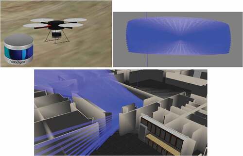
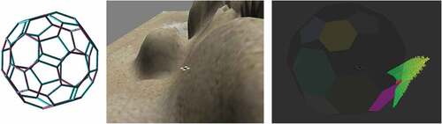
Truncated icosahedron, an object with the shape of a soccer ball, is a formation of twelve pentagons and twenty hexagons. This ball-shape object has ever been formed physically for many UAVs’ purposes such as protective cage (MAHMUD 2021) and moving sport balls (Nitta et al. 2015); but, in this work, we propose a novel way to use a virtual truncated icosahedron structure for UAV, in which the ball shape is visualized to both simplifying point cloud data and at the same time avoiding collisions. The only perception UAV has in this work is from a simulation of Velodyne VLP-16 LiDAR sensor, as can be seen in Figure 3.1. It comes with a 100-meter sensor range, 360°, 30° horizontal and vertical field of views and generates ~300,000 points/second. If we put this huge PCD straight through to the neural networks, it will be too complex to model. If we do fixed-interval sampling to a moderate number, some necessary data may be lost.

Hence, we leverage the ball shape, which is as shown in Figure 3.2, to extract only necessary data for navigation from the mass of the point cloud. The UAV will be covered with the impalpable ball shape structure, which has 32 faces and a radius with the same length as a safe flying distance $p_{radius}$. Sensing observation received from the environment is in the form of vector $\left(f_1,f_2,\dots ,f_{32}\right)$, each $f_i$ denotes a distance between the nearest point cloud, which trespasses into the ball at face $i$, and if $f_i$ is 0, it means that no point cloud trespasses at that face–in other word, there is nothing needed to be taken into account. To calculate $f$, first, we segment only point clouds inside the ball with an implicit equation of the plane. This process is called an inclusion test.

Figure 3.2. Left: Truncated icosahedron structure, Middle: UAV in environment, Right: A UAV’s perception of surrounding objects.

(3.1) $F_i\left(p\right)=a_i{p}_x+b_i{p}_y+c_i{p}_z+d-d=n\times P$(3.1)

Each face of the ball is an oriented plane with a normal vector oriented outside $n_i\left(a_i,b_i,c_i\right)$ and $p$ is the coordinate of the point cloud. $P$ is a known point on the plane. If $F_i\left(p\right)<0$ for at least one, then that point $p$ lies outside the ball and will be ignored. After getting the region of interest of point clouds, next, we find what face the point belongs to by calculating a Euclidean distance of point cloud to the center point of each face $c_i$ as follows:

(3.2) $f_{i=1,32}=\hspace{0.17em}\stackrel{min}{j\in J}\sqrt{{\left(p_{jx}-c_{ix}\right)}^2+{\left(p_{jy}-c_{iy}\right)}^2+{\left(p_{jz}-c_{iz}\right)}^2}$(3.2)

where $J$ denotes the number of point clouds in the ball.

The point belongs to the nearest face and, likewise, the minimum distance point’s value is thus used to represent that face.

Sequential Transition Learning

With the assumption that in a navigation task, the agent should learn from the data which also provides directional insight instead of only one frame, sequential transition was adopted in their works (Kapturowski et al. 2018; Zhang et al. 2020a) and their experimental results showed that it helps improve the performance in various RL tasks. Hence, in this work, the state $s$ which constitutes a transition is a sequence of previous observations. When the agent takes an action in the environment, it receives a current observation $o_t$ which consists of a simplified PCD $\left(f_1,\dots ,f_{32}\right)$, an altitude of UAV $z_t$, two angles of the head’s UAV (or camera direction in headless UAV) with a goal position $h_t$ and a UAV position with a goal position $g_t$. So, an observation has 35 attributes and looks like this $\left(f_1,\dots ,f_{32},z,h,g\right)$. The observation will be stacked up to a fixed-size sequential state in FIFO manner then the state looks like this $\left(o_1,\dots ,o_{p_{frames}}\right)$. $p_{frames}$ is the length of frames in one state.

Augmentative Backward Reward Function

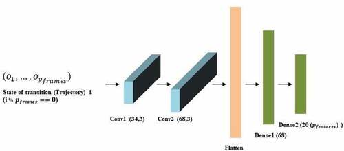
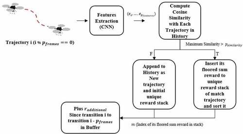
Besides the robust learning models, much research suggests the same thing that augmenting some processes could significantly help the model to converge to optimal policy (Zhang et al. 2020b; Zijian et al. 2020) so we develop a novel reward function called ABR function in this work. The development of this function was motivated by the irrationality of traditional reward functions (Zhang et al. 2020b; Zijian et al. 2020). Traditional reward functions usually have three conditions to give a reward including: when it arrives, when it collides, and others. The irrational part is when they arrive, where the only last transition of the episode will receive a “huge” chunk of reward. Although this part will help increase the success rate, it only works in the setting that is almost constant and very simple due to the fact that it produces a bias on the observation which is similar to the one at the goal. Every time the agent faces this observation, it will be heavily urged to take the same action as the one previously taken at the goal–even though it is bad. So, if the environment is simple enough to hardly find this observation except at the goal area, then the traditional goal reward mechanism can still increase the success rate to convergence. Our hypothesis is that when the agent reaches the goal, it is true that the agent should get more reward than usual to urge this behavior – but not just only the last transition. Every transition in the episode it participated in and contributed to the success (some of them contribute and some not) should be taken into account. The question is how to evaluate the contribution of each transition. Therefore, in ABR, the new goal reward mechanism was developed to dispense goal reward appropriately. With the new mechanism, when the agent arrives at the goal, all transitions in the episode will receive an additional reward ‘proportional’ to its proficiency. ABR consists of the following processes. First, when the agent reaches the goal, all transitions in the episode are fed as input into the backward reward process. Transitions at index $i$, where $i\mathrm{\%}{p}_{frames}=0$ are selected to extract $p_{features}$ features $\left(e_1,\dots ,e_{p_{features}}\right)$ with convolutional neural network (CNN) to be a representative of trajectory $\tau$ of $p_{frames}$ steps motion, the architecture of CNN is as shown in Figure 3.3.

Figure 3.3. Features extraction network structure. The parameters of one-dimensional convolutional layer (Conv1) denote its filters and its kernel size respectively and for the other layers, it denotes dimensionality of output. Each layer’s activation function is Rectified Linear Unit (ReLU).

Next is to calculate the similarity between $\tau$ and each trajectory in history $h$ with a cosine similarity algorithm as follows:

(3.3) $cod\left(A,B\right)=\mathit{1}-\frac{A\cdot B}{\parallel A\parallel \parallel B\parallel }$(3.3)

(3.4) ${\varsigma }_i=\stackrel{max}{j\in J}\left(1-cod\left({\tau }_i,H_j\right)\right)$(3.4)

where $cod$ denotes cosine distance function. $A,B$ = vector. $\varsigma$ denotes cosine similarity between trajectory ${\tau }_i$ and past trajectories. $H$, $J$ = number of trajectories in history.

If ${\varsigma }_i$ is less than similarity threshold $p_{similarity}$ then append ${\tau }_i$ into history $H$ as a new found trajectory pattern. After that, insert floored sum reward $⌊\sum limit{s}_{k=i}^{i-p_{frames}}{r}_k⌋$ of $p_{frames}$ previous transitions into an unique stack of reward of $H$ at index $j$ and sort the stack ascendingly. Additional reward $r_{additional}$ will be added to reward $r$ of transition $i$ until $i-p_{frames}$ in the buffer. The additional reward can be calculated as follows. $r_{additional}=m\times p_{addReward}$ where $p_{addReward}$ denotes some small value, $m$ = index of floored sum reward in the unique stack. The additional reward will be low or high depending on the rank of the sum reward in the unique stack; this mechanism drives the agent to move in a trajectory that gives a larger sum reward than the previous and the whole process of ABR can be illustrated as in Figure 3.4.

Figure 3.4. The process flow of Augmentative Backward Reward function (ABR).

$\begin{array}{rl}& R(s,a)=\left\{\begin{array}{c}{r}_{collided}\mathrm{i}\mathrm{f}\mathrm{c}\mathrm{o}\mathrm{l}\mathrm{l}\mathrm{i}\mathrm{d}\mathrm{e}\mathrm{d}\\ w_1\left(D_{pre}-D_{cur}\right)+w_2\left(-1\left(\left(\left(z-P_{approAlt}\right)\right)/P_{approAlt}\right)\right)\\ w_3\left(1-\left(v_h/180\right)\right)+w_4\left(\left(v_g/180\right)\right)\end{array}\right.+\mathrm{i}\mathrm{f}\mathrm{n}\mathrm{o}\mathrm{t}\mathrm{c}\mathrm{o}\mathrm{l}\mathrm{l}\mathrm{i}\mathrm{d}\mathrm{e}\mathrm{d}\\ & v_h=\left\{\begin{array}{c}360-h\mathrm{i}\mathrm{f}h>180\\ h\end{array}\right.v_g=\left\{\begin{array}{c}360-g\mathrm{i}\mathrm{f}\mathrm{g}>180\\ g\end{array}\right.\end{array}$

(3.5)

The reward function used in this work only has two conditions like this.

where $D_{pre},D_{cur}$ denote the previous and current Euclidean distances between the agent and the goal, $z$ denotes an altitude of UAV, $h,g$ denote angles of the UAV’s head and position to goal, respectively, $p_{approAlt}$ denotes an appropriate altitude or flight level. $W_{1-4}$ denote weight-parameters. If the agent arrives at the goal, it will receive reward from the above function and also all transitions in the episode will receive additional reward from ABR.

Model Architecture

The aim of this work is to develop a universal model, which can navigate the UAV in complex and various environments or whether it be static and dynamic in a realistic fashion. And as mentioned in section 2, it is obvious that only initial DDPG is insufficient to handle the high complex continuous problem like UAV navigation. Therefore, we chose TD3 as a DRL model due to both its efficiency and stability. We will leave the reason for not adding aforementioned techniques like PER in section 4. The main entities in this work consist of: UAV (as an agent), goal, and environment. One exploration episode will end when one of these following conditions occur: 1. An agent reaches within 2 meters radius around the goal and also does not exceed 6 meters in altitude. 2. An agent collides. 3. An agent runs over the limit step. At each time step $t$, the agent receives an observation which is 35 attributes vector of simplified PCD with UAV’s altitude and angles. Subsequently, the agent selects an action that is 4-dimensional vector of three linear velocities and one angular velocity $\left(l_x,l_y,l_z,a_z\right)$ respectively with regards to the current state and policy. After the agent executes the action, the environment returns reward and observation $t+1$ as feedback. Then, the transition including $\left(s_t,a_t,r_t,s_{t+1},d_t,i_t\right)$ is stored into a buffer. 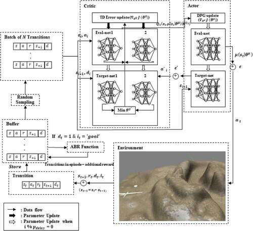During the training, $N$ transitions are sampled from the buffer to form a mini-batch to update parameters in the learning networks. After applying all techniques in 3.1,3.2 and 3.3, the proposed method can be shown as in Figure 3.5 and Algorithm 3.1.

Figure 3.5. The process flow of proposed method in autonomous UAV navigation task. The UAV (agent) ask the actor network for next action and then the critic network will evaluate that selected action.

Algorithm 3.1: TD3 with Sequential transition and ABR Algorithm

Initialize eval-networks of critic $Q_1,Q_2$ and actor μ with random parameters ${\theta }^{Q_1},{\theta }^{Q_2}$ and ${\theta }^{\mu }$. Initialize target-networks with same parameters as in eval-networks $\theta { }^{\mathrm{\prime }}=\theta$

Initialize buffer $B$ with size $p_{buffer}$ and trajectories history $H$

For episode $e$ = 1 to $N$ do

Receive initial observation $o_1$ from $env$ and form state $s$$\left(0,0,\dots ,o_{p_{frames}}\right)$

For $t$ = 1 to $T$ do

Select an action with exploration noise

$a_t=clip\left(\mu \left(s_t|{\theta }^{\mu }\right)+\text{isin},a_{low},a_{high}\right).$

.

Execute $a_t$ and observe reward $r_t$, new observation $o_{t+1}$,

episode status $d_t$.

Generate $s_{t+1}$ by insert $o_{t+1}$ to $s_t$ in FIFO manner.

Store transition $\left(s_t,a_t,r_t,s_{t+1},d_t,i_t\right)$ in $B$.

If $d_t$ == 1 (done) & $i_t$ == ‘goal’ then

Select All transitions $\left(s_i,a_i,r_i,s_{i+1},d_i\right)$ in $e$ from $B$.

For $k$ = 1 to $t/p_{frames}$ do

$l$ = $k$ + $p_{frames}$.

$\left(e_1,\dots ,e_{p_{features}}\right)={\tau }_k$ = trajectory extracted from $s_l$ with CNN.

Find similarity ${\varsigma }_k=j\in J\left(1-cod\left({\tau }_k,H_j\right)\right)$.

if ${\varsigma }_k<p_{similarity}$ then

Append ${\tau }_k$ to $H$.

end if

Calculate floored sum reward $R=\sum _{j=l}^{l-p_{frames}}{r}_j$.

Insert $R$ to unique reward stack of $H_j$ & sort stack then $m$ is return index.

$r_{l,l-p_{frames}}+=m\times p_{addReward}$

end for

end if

Sample mini-batch of $N$ transitions $\left(s_i,a_i,r_i,s_{i+1},d_i\right)$ from $B$ randomly.

${a{ }^{\mathrm{\prime }}}_i=clip\left(\mu { }^{\mathrm{\prime }}\left(s_{i+1}|{\theta }^{\mu { }^{\mathrm{\prime }}}\right)+\epsilon ,a_{low},a_{high}\right)$, $y_i=r_i+\gamma \left(1-d_i\right)j=1,2Q\mathrm{\prime }j{s}_{i+1},a\mathrm{\prime }i|\theta Q\mathrm{\prime }j$.

Update critic ${\mathrm{\nabla }}_{{\theta }_j^Q}\left({\theta }_j^Q\right)=\frac{1}{N}\sum _{i=1}^N{\mathrm{\nabla }}_{{\theta }_j^Q}{\left(y_i-Q_j\left(s_i,a_i|{\theta }^{Q_j}\right)\right)}^2$.

if $t$ mod $p_{updateDelay}$ == 0 then

Update actor ${\theta }^{\mu }$ using deterministic policy gradient

${\mathrm{\nabla }}_{{\theta }^{\mu }}J\left({\theta }^{\mu }\right)=\frac{1}{N}\sum _{i=1}^N{\mathrm{\nabla }}_{{\theta }^{\mu }}{Q}_1\left(s_i,\mu \left(s_i|{\theta }^{\mu }\right)|{\theta }^{Q_1}\right).$

Update target networks

${\theta }^{Q{ }^{\mathrm{\prime }}}=p_{tau}{\theta }^Q+\left(1-p_{tau}\right){\theta }^{Q{ }^{\mathrm{\prime }}}$, ${\theta }^{\mu { }^{\mathrm{\prime }}}=p_{tau}{\theta }^{\mu }+\left(1-p_{tau}\right){\theta }^{\mu { }^{\mathrm{\prime }}}$.

end if

if $t>p_{limitStep}$ or $d_t$ == 1 (done) then

break loop.

end if

end for

end for

Experiments

To approach the real-world adoption more closely, the proposed method was trained under the condition that is as realistic as possible. As aforementioned, it is unaffordable to learn from raw LiDAR sensing data hence, all UAV experiments in this work are operated under point cloud simplification with Truncated Icosahedron structure. At each episode, the positions of UAV and the goal were randomly set. The success rate (a probability of the UAV reaching the goal for the last 500 episodes) was used to measure the performance of each method. And in this section, several experiments are conducted to compare the performances in UAV navigation tasks between the proposed method and related state-of-the-art methods.

Experimental Setting

In this work, the UAV control was operated via Robot Operating System (ROS) (Stanford Artificial Intelligence Laboratory et al. 2018) and the data in aspects of UAV were visualized by Rviz (Kam et al. 2015). In terms of environment, GAZEBO framework was in charge of it all. The programming language used to implement the proposed method was Python3. All processes ran on a laptop computer with Ubuntu 20.04, Core™ i7 CPU @2.20 GHz, GeForce GTX 1050 Mobile Graphic chip and 32 GB memory. List of attributes and hyper-parameters for this work are shown in .Table 4.1

Table 1. Attributes and Hyper-parameters for this work.

No.	Name	Symbol	Value
1	UAV	-	Quadrotor
2	LiDAR sensor	-	Velodyne vlp
3	Environment	-	1200 $m^2$
4	Discount factor	$\gamma$	0.99
5	Soft update rate	$p_{tau}$	0.005
6	Noise bound	$c$	0.5
7	Action limit	$a_{low},a_{high}$	-2,2
8	Number of frames in one state	$p_{frames}$	3
9	Number of features extracted from one state	$p_{features}$	20
10	Similarity threshold	$p_{similarity}$	98%
11	Additional reward multiplier	$p_{addReward}$	0.1
12	Delay to slow the update of actor and target networks	$p_{updateDelay}$	2
13	Reward when collide	$r_{collided}$	-50
14	Appropriate altitude or Flight level	$p_{approAlt}$	3.5 m
15	Size of buffer	$p_{buffer}$	${10}^6$
16	Weight-parameters in reward function	$w_{1-4}$	8,1,1,0.5 respectively
17	Radius of Truncated icosahedron structure, Safe flying distance	$p_{radius}$	4 m
18	Maximum number of steps per episode	$p_{limitStep}$	300
19	Batch size	$N$	100
20	Traditional reward function: goal reward, collision punishment (In case “other”, Formula 3.5)	-	50,-50
21	Small reward given to all transitions in success episode of equal goal reward function	-	1

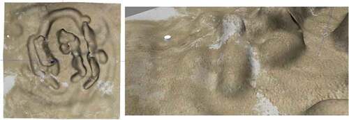
Figure 4.1. The 3D static simulation environment. Left: Top view of all whole map. Right: Main view of center of map. The white cylinder is goal point.

Experimental Results

Training In Static Environments

The 5000 episodes training of five methods: 1. DDPG with Sequential transition and Traditional Reward function, 2. TD3 with Sequential transition and Traditional Reward function, 3. TD3 with Sequential transition and No Goal Reward function (traditional reward function but no goal reward when the agent reached the goal point), 4. TD3 with Sequential transition and Equal Goal Reward function (traditional reward function but gives a small equal reward to all transitions instead of a chunk of goal reward to a last transition), 5. TD3 with Sequential transition and ABR (proposed method) were conducted on the static environment, valley, as shown in Figure 4.2.

Figure 4.2. Experimental result in static environment. Left: Average success rate that UAV reach the goal point. Right: Average collision rate that UAV collide with environment surface. (The figure is designed for color version).

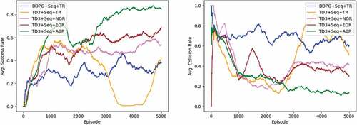
Figure 4.3. The 3D dynamic simulation environment. Left: Top view of all whole map. Right: Main view of center of map.

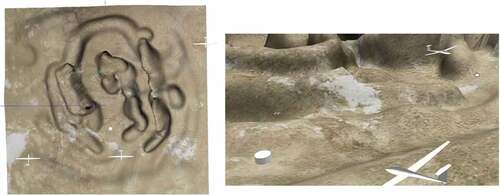
Figure 4.4. Experimental result in dynamic environment. Left: Average success rate. Right: Average collision rate. (The figure is designed for color version).

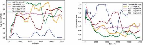
The experimental results demonstrate that DDPG’s performance was lower than that of TD3. DDPG achieved a 37.8% success rate, which was almost the same value as in the high complexity environment experiment of Hu et al. 2020, and the highest is 46% at around episode 3600. In terms of TD3, TD3 with traditional reward function achieved 42.2% and 57.3% highest at around episode 1300. It is noticeable that after episode 3500 of TD3, the success rate dramatically falls down according to the increase of collision rate. From the observation, we found that at that period, the UAV changed the behavior to fly as close as designated altitude $p_{approAlt}$, it may try to earn more rewards but nonetheless this raises the risk of collision instead. However, performances of these two methods are still considered as low if considering the real-world adoption. The success rate was increased by around 10% after we cut off the chunk of goal reward in the traditional reward function, TD+Seq+NGR achieved 53.6%. This result was according to our hypothesis that a chunk of goal reward produces bias to the observation similar to the one at goal. Next, we tried changing the chunk of goal reward into giving equal small reward to all transitions in the episode in which the agent reached the goal point. This simple goal reward dispensation helps stimulate the agent reaching the goal more often, the success rate was boosted to 69.2%. But when we used the more rational goal reward dispensation, ABR, the success rate was tremendously increased to 84.8%.

Training In Dynamic Environments

Besides complex geography, what it should be concerned in real world is moving objects that may obstruct the UAV’s flight like birds and planes. Consequently, we added three planes having speed and flight level close to UAV’s into the environments as shown in Figure 4.3.

As expected and shown in Figure 4.4, the success rate of UAV reaching the goal falls down to 61.6% when the UAVs are trained in dynamic environments with the proposed method and reach the highest 74% at around episode 2900 – the same situation as in episode 1300 occurs again, after episode 2900. The UAV tried to maintain the altitude at $p_{approAlt}$, which is the same altitude level as planes and as a result the collision frequently occurs then it leads to decrease of success rate. Contrarily, the result of TD3 with traditional reward function was 37% success rate, which is slightly lower than its result in the static environments, but the highest is 73.8% which is almost the same as of the proposed method. The success rates of TD3 with no goal reward and equal goal reward function were higher than that of the traditional reward function: 47.8% and 55%, respectively. The success rate of the DDPG method was only 0.6%; it looked unsteady and never reached even 20%.

TD3 with ABR in Other Tasks

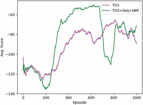
To make sure that the proposed method is robust, we tested it on BipedalWalkerHardcore, a testbed for RL, in which it has many similar componentsm such as UAV navigation tasks. The aim of BipedalWalkerHardcore is to move a robot forward as far as possible by having obstacles like pitfall, ladder and stump existing in front. The observation robot receives 10 lines of LiDAR sensor and velocity in various angles. Due to the fact that there is no target point in this task thus we defined a certain episodic reward as the target and goal. The result of 1000 episodes of training, which shown in Figure 4.5, indicates that just changing reward function to ABR in TD3 can improve the episodic reward from −89.61 to −70.91 (the average of the last 100 episodes).

Figure 4.5. Experimental result of TD3 method and TD3+Seq+ABR method (Proposed) in other navigation task, BipedalWalkerHardcore. (The figure is designed for color version).

Conclusion

This work proposed two novel methods to make Autonomous UAV Navigation closer to real world adoption. First, we leverage the truncated icosahedron structure (a soccer ball-like object) to extract only necessary data from precise LiDAR sensor data which is unaffordable for deep neural networks to learn. As proved in the past (Kapturowski et al. 2018; Zhang et al. 2020a), sequential transition was adopted in this work to let the agent learn rich data which is not laconic. Second, we address the problem of having bias at goal state in the traditional reward function with rational goal reward dispensation in ABR function. The experimental results indicate palpably that TD3 is better than DDPG in high state-action spaces and extra rewards could help stimulate the agent reaching the goal point. On the other hand, if the goal reward mechanism is irrational, it will result in harm instead. This influence can be observed in the experimental results of TR, EGR, and ABR that the success rates are higher according to the level of rationality. The proposed method achieved 84.8% success rate to navigate UAVs to the goal in static environments and 61.6% for dynamic environments. In addition, we have tested the proposed method on another navigation task, BipedalWalkerHardcore and the result was as expected in which adding ABR to TD3 improves the episodic reward from −89.61 to −70.91. This is evident that the proposed method is robust.

However, we still have found the problem that the agent is apprehensive against risky scenes, in all methods we have tested including the proposed method. When the agent faces risky scenes such as high hills in late episodes of training, it will move back and forth repeatedly until running out of quota steps. This behavior seems like the way the agent used to avoid punishment and lead to stuck in local optima. The video of our experiments is available at https://youtu.be/WYpYSG0t7oU.

In the future, we intend to improve our method to gain more success rate and less collisions in even more challenging environments.

Disclosure Statement

No potential conflict of interest was reported by the author(s).

References

- A, M., R. Hado P van Hasselt, and R. S. Sutton. 2014. Weighted importance sampling for off-policy learning with linear function approximation. Neural Information Processing Systems. Curran Associates, Inc. https://proceedings.neurips.cc/paper/2014/hash/be53ee61104935234b174e62a07e53cf-Abstract.html
- Bellman, R. 1957. A markovian decision process. Indiana University Mathematics Journal 6 (4):679–2339. doi:10.1512/iumj.1957.6.56038.
- Erke, S., D. Bin, N. Yiming, Q. Zhu, X. Liang, and Z. Dawei. 2020. An improved a-star based path planning algorithm for autonomous land vehicles. International Journal of Advanced Robotic Systems 17 (5):172988142096226. doi:10.1177/1729881420962263.
- Falanga, D., K. Kleber, and D. Scaramuzza. 2020. Dynamic obstacle avoidance for quadrotors with event cameras. Science Robotics 5 (40):eaaz9712. doi:10.1126/scirobotics.aaz9712.
- Fujimoto, S., H. van, and D. Meger. 2018. Addressing function approximation error in actor-critic methods. ArXiv organization. https://arxiv.org/abs/1802.09477
- Hajdu, C., and Á. Ballagi. 2020. Proposal of a graph-based motion planner architecture. 11th IEEE International Conference on Cognitive Infocommunications (CogInfoCom) Online on MaxWhere 3D Web. September 1, 2020. doi:10.1109/CogInfoCom50765.2020.9237891.
- Hou, Y., and Y. Zhang. 2019. Improving DDPG via prioritized experience replay. https://cardwing.github.io/files/RL_course_report.pdf
- Kam, H. R., S.-H. Lee, T. Park, and C.-H. Kim. 2015. RViz: A toolkit for real domain data visualization. Telecommunication Systems 60 (2):337–45. doi:10.1007/s11235-015-0034-5.
- Kapturowski, S., G. Ostrovski, J. Quan, R. Munos, and W. Dabney. 2018. Recurrent experience replay in distributed reinforcement learning. Openreview.net. September 27, 2018. https://openreview.net/forum?id=r1lyTjAqYX
- Koenig, N., and A. Howard. 2004 Design and use paradigms for Gazebo, an open-source multi-robot simulator. 2004 IEEE/RSJ International Conference on Intelligent Robots and Systems (IROS) (IEEE CatNo.04CH37566) Sendai, Japan. Accessed October 20, 2019. doi:10.1109/iros.2004.1389727.
- Kolar, P., P. Benavidez, and M. Jamshidi. 2020. Survey of datafusion techniques for laser and vision based sensor integration for autonomous navigation. Sensors 20 (8):2180. doi:10.3390/s20082180.
- Konda, V. R., and J. N. Tsitsiklis. 2003. OnActor-critic algorithms. SIAM Journal on Control and Optimization 42 (4):1143–66. doi:10.1137/s0363012901385691.
- Lillicrap, T. P., J. J. Hunt, A. Pritzel, N. Heess, T. Erez, Y. Tassa, D. Silver, and D. Wierstra. 2015. Continuous control with deep reinforcement learning. ArXiv.org. https://arxiv.org/abs/1509.02971.
- MAHMUD, A. L. 2021. Development of collision resilient drone for flying in cluttered environment. Graduate Theses, Dissertations, and Problem Reports (January). doi:10.33915/etd.8022.
- Mnih, V., K. Kavukcuoglu, D. Silver, A. Graves, I. Antonoglou, D. Wierstra, and M. Riedmiller. 2013. Playing atari with deep reinforcement learning. ArXiv.org. https://arxiv.org/abs/1312.5602.
- Nitta, K., K. Higuchi, Y. Tadokoro, and J. Rekimoto. 2015. Shepherd pass. Proceedings of the 12th International Conference on Advances in Computer Entertainment Technology Iskandar, Malaysia, November. doi:10.1145/2832932.2832950.
- Schaul, T., J. Quan, I. Antonoglou, and D. Silver. 2015. Prioritized experience replay. ArXiv organization. https://arxiv.org/abs/1511.05952.
- Silver, D., G. Lever, N. Heess, T. Degris, D. Wierstra, and M. Riedmiller. 2014. Deterministic policy gradient algorithms. Proceedings.mlr.press. PMLR Bejing, China. January 27, 2014. https://proceedings.mlr.press/v32/silver14.html.
- Stanford Artificial Intelligence Laboratory et al.2018. Robotic operating system (version ROS Melodic Morenia) https://www.ros.org.
- Sutton, R., and B. En A. G 1999 . Reinforcement learning. Journal of Cognitive Neuroscience 11 01 1999:126–34
- Tan, F., P. Yan, and X. Guan. 2017. Deep reinforcement learning: from Q-learning to deep Q-learning. Neural Information Processing 475–83. doi:10.1007/978-3-319-70093-9_50.
- Youn, W., K. Hayoon, H. Choi, I. Choi, J.-H. Baek, and H. Myung. 2020. Collision-free autonomous navigation of a small UAV using low-cost sensors in GPS-denied environments. International Journal of Control, Automation, and Systems 19 (2):953–68. doi:10.1007/s12555-019-0797-7.
- Zhang, L., S. Han, Z. Zhang, L. Lefan, and S. Lü. 2020a. Deep recurrent deterministic policy gradient for physical control. Artificial Neural Networks and Machine Learning –ICANN 2020:257–68. doi:10.1007/978-3-030-61616-8_21.
- Zhang, Q., M. Zhu, L. Zou, L. Ming, and Y. Zhang. 2020b. Learning reward function with matching network for mapless navigation. Sensors 20 (13):3664. doi:10.3390/s20133664.
- Zijian, H., K. Wan, X. Gao, Y. Zhai, and Q. Wang. 2020. Deep reinforcement learning approach with multiple experience pools for UAV’s autonomous motion planning in complex unknown environments. Sensors 20 (7):1890. doi:10.3390/s20071890.