Intelligence based Accurate Medium and Long Term Load Forecasting System

ABSTRACT

In this study, we aim to provide an efficient load prediction system projected for different local feeders to predict the Medium- and Long-term Load Forecasting. This model improves future requirements for expansions, equipment retailing or staff recruiting to the electric utility company. We aimed to improve ahead forecasting by using hybrid approach and optimizing the parameters of our models. We used Long Short-Term Memory (LSTM), Convolutional Neural Network (CNN), Multilayer perceptron (MLP) and hybrid methods. We used Root Mean Square Error (RMSE), Mean Absolute Percentage Error (MAPE), Mean Absolute Error (MAE) and squared error for comparison. To predict the 3 months ahead load forecasting, the lowermost prediction error was acquired using LSTM MAPE (2.70). For 6 months ahead forecasting prediction, MLP gives highest predictions with MAPE (2.36). Moreover, to predict the 9 months ahead load forecasting, the highest prediction has been attained using LSTM in terms of MAPE (2.37). Likewise, ahead 1 years MAPE (2.25) was yielded using LSTM and ahead six years MAPE (2.49) was provided using MLP. The proposed methods attain stable and better performance for prediction of load forecasting. The finding indicates that this model can be better instigated for future expansion requirements.

Introduction

Maintaining the stable operation of Power systems and electricity dispatching instructions requires load forecasting (Singh and Dwivedi 2018). Volatility and uncertainty in electric loads are produced by external variables (Ertugrul 2016)(ZHANG et al. 2018). Individual residential loads, in contrast to aggregated loads, are less predictable due to the lack of load smoothing (Ranaweera, Hubele, and Karady 1996). Customers also participate in demand response on an ad hoc basis, complicating residential load forecasting (He et al. 2016b)(AMJADY and KEYNIA 2009). The electric load demands according to the needs of residential, industrial, special events, seasonal and government and private sectors requires powerful automated tools to accurately forecast ahead demands.

Machine learning is less effective when dealing with large amounts of data and recent studies show that researchers not considered long-term forecasting with these methods. Deep learning (. Szegedy et al. 2015)(L.-C. Chen et al. 2018) appears to be a viable method for properly handling large amounts of data. Deep learning features a multi-layer nonlinear network topology that allows for complicated feature abstraction and nonlinear mapping (Qiu et al. 2014). By supervised fine-tuning of the parameters and multilayer unsupervised training, a deep belief network (DBN) may extract features (Zheng et al. 2014). The mining of spatial correlations is possible with convolutional neural networks (CNNs) (S. Yang et al. 2015). Image recognition (Kollia and Kollias 2018), renewable energy forecasting (Tian et al. 2018), and load forecasting (Khotanzad, Afkhami-Rohani, and Maratukulam 1998a) all use CNNs. In Shivarama Krishna and Sathish Kumar (2015), a combination of CNN and load range discretization was effectively employed in probabilistic load forecasting. Long short-term memory network (LSTM) is another exemplary deep learning model, which is a variation of the recurrent neural network (RNN) and can deal with time series implied long-term dependencies (Kong et al. 2019). Several LSTM-based load forecasting algorithms have been proposed (Han et al. 2019)(Park, Yoon, and Hwang 2019)(LeCun, LeCun and Bengio 1995)(Hochreiter, Schmidhuber, and J 1997). An LSTM-based load forecasting strategy for a single user was employed in Oord et al. (2016), and a careful comparison with benchmark approaches indicated the method’s benefit. LSTM is chosen as the prediction model’s foundation because of the proposed temporal link in the load series. Despite this, LSTM treats all inputs the same, neglecting the reality that input vectors have varying roles in prediction at different time steps (He et al. 2016a).

Load forecasting is an approach that is implemented to foresee the future load demand projected on some physical parameters such as loading on lines, temperature, losses, pressure, and weather conditions, etc. Load forecasting is a course of action followed by electric corporations to foresee electrical potential required to stabilize supply and load demands on the continuous basis. It is required for the established working of the industries that run electrically. Load forecasting within energy management network could be classified into four types as per distinctive length of forecasting intervals (Singh and Dwivedi 2018): (i) very short-term load forecasting (VSTLF) predicts load just for small time span; (ii) short term load forecasting (STLF); it forecasts load starting from 24 hours prolonging to 1 week; (iii) medium term load forecasting (MTLF), it forecasts load over few weeks to number of few months or till one year; and (iv) Long Term Load Forecast (LTLF) forecasts load up to several years. In this study, we emphasize on MTLF and LTLF which is fundamental for controlling, planning for power systems, evaluation of interchange, assessment of security, reliability analysis along with spot value estimation [2] (ZHANG et al. 2018) which prompts the higher precision necessity as opposed to long-term forecast.

Many new approaches have been employed for the objective of load forecasting such as fuzzy logic, Artificial Intelligence (AI), etc. Utilization of AI advancements to understand STLF is turning out to be widely applicable these days. Numerous applications worldwide are being benefited with newly created AI based frameworks. Fuzzy logic has been employed to integrate load and weather data by (Ranaweera, Hubele, and Karady 1996). These fuzzy principles were acquired by the historical data with the utilization of a learning-type calculation (Ranaweera, Hubele, and Karady 1996). In Y. He et al. (2016) the authors presented an architecture for evaluating the vulnerability of load and obtaining further information about potential subsequent loads, after which a neural framework has been employed to remake the quantile regression archetype for developing probabilistic forecasting techniques. In AMJADY and KEYNIA (2009), authors present a hybrid forecasting model for STLF based on wavelet transition and neural system, as well as an evolutionary algorithm. The authors of Ghofrani et al. (2015) presented a combination of Bayesian Neural Network (BNN) and Wavelet Transform (WT) to generate the load characteristics for BNN formulation in a comparative technique. This approach employed a weighted total of the BNN yields to anticipate the load for a particular day. An STLF model suggested by Fan, Peng, and Hong (2018) combines Phase Space Reproduction (PSR) calculations with the Bi-Square Kernel (BSK) regression model in one of the previous hybrid models. To boost the forecast’s unshakable efficiency, a phase space reconstruction technique might be utilized in this model to detect the developmental trends of historical load, as well as the inserted significant highlights data. The BSK architecture, on the other hand, connects the spatial assemblies between regression points and their neighbors to obtain rotatory rule guidance and alarming impact in each measurement. STLF (Fan, Peng, and Hong 2018) was able to successfully create and use the proposed model, which included multi-dimensional relapse. Mamlook et al. used a fuzzy logic controller-based hourly system to estimate the impact of numerous restricted criteria, including the atmosphere, time, load historical summation of data, and random upsetting influences, as well as overload forecasting for fuzzy sets utilizing the age approach, in Mamlook, Badran, and Abdulhadi (2009). WT divided the time stream into segments in this study, then anticipated each segment using a neural network and an evolutionary algorithm.

Deep convolutional neural networks are employed for a vast array of tasks, including medical image analysis (Litjens et al. 2017) and image classification (Glorot, Bordes, and Bengio 2011). Feature detector units are placed in layers in a deep learning architecture. Lower layers detect simple features, which are sent into higher layers, which detect more complex features. Convolution neural networks (CNNs) (LeCun, Bengio, and Hinton 2015) are a type of neural network. In comparison to standard feed forward neural networks, the structural elements (i.e., neurons) are significantly reduced. The deep learning convolutional neural network using transfer learning methods has been validated in earlier works (Shin et al. 2016; H. Chen et al. 2015; S. Gupta et al. 2014; S., 2015; Shin, Lu, and R.m.s 2015) and is widely utilized in imaging databases (S. Gupta et al. 2014; S., 2015), neuroimaging (A. Gupta, Ayhan, and Maida 2013), MRI, CT (Computed Tomography), (H. Chen et al. 2015) and ultrasound images (Cao et al. 2018).

In another method, the research investigating about utilizing AI for STLF was given by Metaxiotis et al. (2003). Lately, Convolutional Neural Networks (CNNs) have shown better execution in forecasting. CNNs were presented by Fukushima in its straightforward structure (Fukushima and Miyake 1982). Afterward, authors of LeCun et al. (1999) introduced the current type of CNNs with further developed ideas. Since their inception, the CNNs have met numerous upgrades and augmentations, for example, max pooling sheets and layers along with bunch normalization presented by (Sermanet et al. 2013). In spite of the fact that CNNs are fruitful for the forecasting (Abdulnabi et al. 2015; Levi and Hassncer 2015), one of the principle issues of utilizing them over other profound neural systems strategies is over-fitting (Xie et al. 2016). As Burnham characterized (Burnham and Anderson 2004) over-fitting is the creation of an examination that relates too intently or precisely to a specific data set and may in this manner neglect to fit added data or dependably foresee future perceptions. There are a few strategies to keep away from or lessen over-fitting in the scenario of deep learning designs profound learning models, for example, data augmentation methods, utilizing regulations entitles in the intended function as well as batch normalization (Goodfellow, Bengio, and C.A 2016). A few procedures are explicitly intended for CNN models, for example, incorporating a pooling layer in the design (Guo et al. 2016). In rundown, CNN is a decent approach for STLF applications, in so far as over-fitting could be controlled.

STLF has been the vital zone of research utilizing statistical techniques along with Artificial Neural Network (ANN). Statistical methodologies incorporate the Autoregressive Integrated Moving Average (ARIMA) (Yuan, Liu, and Fang 2016), double-seasonal Holt Winters exponential smoothing (Taylor 2003) along with PCA-based Linear Regression (Bair et al. 2006). Currently, ANN-derived methodologies have attained extensive consideration in electrical load forecasting. There has been a change in model design in an ANN system that relies on both forecasting length and the information required to make the forecast. There are two types of successions: one is univariate and the other is multivariate. Models that use univariate datasets will be basic, small in size, and efficient trainers in general; nevertheless, they will have low precision. On the contrary, models dependent over multivariate datasets happen to be computationally slow in practice. In order to address such issues, first of all the preprocessing of a provided dataset modified to multi-bivariate successions to successfully get familiar with the characteristics, which could be extricated from the information taken out of individual context. A new hybrid model has been exploited to precisely forecast n-day depiction demand requirement. Particularly, the suggested hybrid network comprises of multi-Long Short-Term Memory (LSTM) layers as well as CNN layer. Analyzing multi-LSTM layers, from every input, there is a separation of features by each layer, contained a bi variate succession, and caters these characteristics to a CNN layer to attain an n-day profile. The recommended hybrid model is focused on wide forecasting concerns taking all short-term strata time associated granularities (minutes, hours, days and so on). By proposing a bi variate-based setting learning strategy, the proposed hybrid model structure combines the productivity of multi-LSTM in distinguishing features out of multiple setting data with the capacity of CNN.

Many of the strategies used to forecast power requirements have incorporated Recurrent Neural Network (RNN) based LSTM, that utilized on Natural Language Processing (NLP) and time series data (Krizhevsky, Sutskever, and Hinton 2012; Sundermeyer, Ney, and Schluter 2015; Wen et al. 2015). Specifically, CNN have delivered highly extreme classification and identification execution within the field Personal Computer (PC) vision and the recognition of pattern (. Szegedy et al. 2015; L.-C. Chen et al. 2018; Krizhevsky, Sutskever, and Hinton 2012) and have additionally been exhibited to be powerful in different fields including TS data, for example, language information, pattern data related to human behavior, power load data and so on (Qiu et al. 2014; Yang et al. 2015a; Zheng et al. 2014).

These days, hybrid energy framework has gotten progressively mainstream in the power industry. The major motive of the trend is growingly decrease of power stockpiling cost and the improvement of computerized interrelation, empowering real time observation and establishment of smart grid. In addition, hybrid energy framework is contemplating as probably the best arrangement in handling irregularity happening by most sustainable power scheme plans comprising solar energy and wind power. For instance, in solar-based photovoltaic, power is possibly conveyed while getting adequate solar transmittance. As a result, a great extent of examination has been led so as to give the best plan of hybrid energy framework (Shivarama Krishna and Sathish Kumar 2015).

However, in view of the ongoing publications (Han et al. 2019; Kong et al. 2019; Park, Yoon, and Hwang 2019; Tian et al. 2018), deep learning techniques exhibit the utmost efficient performance beside presentation by AI based solutions. The major reasons for the deep learning predominance come in the first place, deep learning doesn’t exceptionally depend on feature-based engineering and the hyper boundaries tuning is generally simpler contrasted with rest of the data-driven models. The other one is the accessibility of enormous datasets, the point at which the deep learning might correctly plan the contributions to the specific yield by building composite relations between the surfaces in the system on massively positioned data. Additionally, as the accessibility of GPU equal calculation and strategies giving loads sharing such as CNN (LeCun, LeCun and Bengio 1995), computational pace related to the deep learning architectures get significantly quicker.

In light of the prevalence in the field of deep learning, our work suggests a technique in load forecasting task, particularly MTLF, to foresee the hourly power utilization by utilizing deep learning calculations that is blend adaptation of CNN, expanded causal surplus CNN along with LSTM (Hochreiter, Schmidhuber, and J 1997). Dilated causal remaining CNN is motivated through Wavenet design (Oord et al. 2016), that is renowned for generation of audio along with residual system (He et al. 2016b) with gate-activation work. This design will gain proficiency with the pattern dependent on long sequential input while Long Short-Term Memory layer functions as a model’s output self-revision that relates the result of Wavenet model with ongoing load demand tendency.

The principle commitment of this examination is that we suggest a new model using a blend of widened causal surplus CNN as well as LSTM using long and short successive information and fine drawn method. The extraction of the outer component or feature determination data is excluded from this examination. In addition, this exploration just considers time index data as an outside factor data, making it simple to be looked at as a standard architecture for future examination.

To enhance the versatility of our suggested model depiction, two different situations related to model testing are examined. The first situation is utilizing the testing dataset carrying indistinguishable appropriation with the approval information set, on the other hand the second is utilizing informational index having obscure dispersion. As a correlation, our suggested model outcomes are compared and the exhibition of the model from Kong et al. (2019) Tian et al. (2018) along with the benchmarked wavelet (Oord et al. 2016). The simulation outcome shows that our model yielded better results than previous machine and neural network methods with less prediction error.

Recently, researchers utilized hybrid methods of CNN models for prediction of time series problems. Xu et al. (Xu et al. 2022) employed particle swarm optimization (PSM) in LSTM to improve the ahead prediction of short-term flood forecast. The researchers (Stefenon et al. 2020) applied LSTM with Adaptive Neuro-Fuzzy Inference System (ANFIS) to predict fault in electrical power insulator. Moreover, Rodrigues Moreno et al. (2020) employed LST with multi-stage decomposition model to predict ahead multi-step wind speed forecasting. The researcher (Cho and Kim 2022) applied hybrid method i.e. weather Research and Forecasting hydrological modeling system (WRF-Hydro) with LSTM to improve streamflow prediction. The researchers (Cho and Kim 2022) applied efficient bootstrap stacking ensemble learning method to improve the wind power generation forecasting.

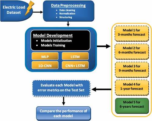
A schematic diagram of an electric load forecasting system for short- and medium-term demand forecasting is shown in Figure 1. The MTLF is used to schedule power systems for periods ranging from three months to six year. We calculated the MTLF for the next 3 months, 6 months, 9 months, 1 year and 6 years in this case. An optimal model based on Multilayer Perceptron (MLP), LSTM, CNN, and CNN + LSTM has been presented in this work. On the test collection, the output was calculated using standard performance error metrics including RMSE,MSE, MAE, MAPE and R-squared. Moreover, MTLF ahead load forecasting is computed and efficiency is assessed according to the error in expected and real load demands.

Figure 1. Schematic diagram of electric load forecasting system.

Smart Grids are developing, creating, and profiting by the advancement of data and correspondence advances and are progressively turning into an effective and powerful framework. In these environments, power conservation frameworks are fabricated to observe, accelerate, and dominate the vitality market. Demand Management contemplated an indispensable segment of the power management architectures; gives the way to settle on pertinent choices on the trading of electrical vitality between various elements of the electrical network of grids by guaranteeing the solidity along with steady quality of the proper functioning of the electrical infrastructures (Murthy Balijepalli et al. 2011).

The currently prevailing power grids are showing a rapid growth, producing numerous apprehensions regarding environment, effective use and supportability along with energy autonomy. Load forecasting framework has the basic role for power demand supply organizations (Chan et al. 2012; Faria and Vale 2011; Moslehi and Kumar 2010).

Precise and definitive forecasting strategies can add to:

• Supply-demand designing

• Strengthen the dependability of electric grid qualities by getting it trouble free for administrators to intent along with compelled planned conclusions for vendors.

• Optimizing power load which is required on high occasions by guaranteeing that energy supplied by manufacturer is decreased.

• The amicable integration of sustainable resources assists with accomplishing natural along with monetary targets.

• Save working and preservation costs by maintaining systematic framework at a lesser price and decreasing system.

Time series data on load forecasts from January 1, 2017 to May 31, 2020 (41 months), we computed next 3 months, 6 months, 9 months, 1 year and 6 years ahead forecasting using the proposed methods. In the past few decades, due to the rapid surge in the wind production of electricity, the capacity of the

wind power has been increased almost four-fold from 4.3 GW to 203.5 GW. The power systems in their growth and complexity, several factors become influential to the electric power production and consumption. The electric utilities’ basic difficulty is to maximize the long-term and short-term operation system efficiency. Load forecasting has become a critical challenge for electric utilities in order to promote economic development and fulfil power needs in the future. The development of a strategy for power supply, finance planning, electricity management, and market search can all benefit from an accurate load forecasting system (Bozchalui et al. 2012), (Khator and Leung 1997). The STLF is used in the power systems planning for unit commitment and dispatch, potential for cost-effective and safe power system service (1 hour-72 hours up to one week), while medium-term forecasting ranging from one days to one year is used to plan maintenance of the wind farms, outage of thermal generation, unit commitment, storage operation and to schedule grin maintenance of energy, it also coordinates the delivery of fuel and the repair of equipment. In power system planning, long-term load forecasting (more than a year ahead) is used (Khator and Leung 1997).

Rest of the paper is arranged as: Section 2 presents the materials and methods. Results are discussed in section 3 and discussion is made in section 4. Conclusions are discussed in section 5. This work is related to the various case studies of the authors such as published in Mehmood Butt et al. (2021).

In this analysis, we used dataset of electric power consumption collected on hourly basis between 1st January 2017 to 31, May 2020 (41 months). We split the dataset into two sets: train and test with respect to testing period using 10-fold cross validation, i.e. for model 1 we used the data of last three months as a test data and previous data was consider as training data. Cross-validation method is used to train and test the data simultaneously for validation purposes. Similarly for model 2–4, we used last 6,9 and 12 months data as test set and previous data was considered as training data. Then we trained MLP, 1D-CNN, LSTM and CNN+LSTM with respect to train set. After that, we evaluated and compared the performance of each method with different error metrics on all test sets.

LSTM

We create an LSTM model with one LSTM layer of 64 neurons and ” RELU” as an activation function. After that we added four dense layers, where first three layers contains 32, 16 and 8 neurons respectively with “RELU” activation function. The final layer which also acts as the output layer contains 1 neuron. Finally, we compiled our model using optimizer = “ADAM” and train it for 100 epochs with a batch size of 24.

Conv1D

For Conv1D we defined 64 filters and a kernel size of 2 with “RELU” as an activation function. In order to reduce the complexity of the output and prevent over fitting of the data, we used Max pooling layer after a CNN layer with size of 2. Moreover, four dense layers were added from which first three layers contains 32, 16 and 8 neurons respectively with “ RELU“ activation function. The final output layer contains 1 neuron. Lastly, we used mean squared error loss function in this model was compiled with “ADAM” optimizer and then fit for 100 epochs by, and a batch size of 24 samples is used.

MLP

With MLP, the first four dense layers of model consist of 64, 32, 16 and 8 neuron and ”RELU” as an activation function. In addition, the final dense layers were added with 1 neuron for output. Lastly, the model was fit using the efficient ADAM optimization algorithm and the mean squared error loss function for 100 epochs with batch size of 24.

CNN± LSTM

For this hybrid approach, we defined 64 filters and a kernel size of 2 with “RELU” as an activation function. Following this we then add Max pooling layer, then output is flattened to feed into LSTM layers contains 64 neurons and ” RELU” as an activation function. After that we added four dense layers, where first three layers contains 32, 16 and 8 neurons respectively and final output layer, contains 1 neuron. At the end, we compiled our model using optimizer = “ADAM” and train it for 100 epochs with a batch size of 24.

Material and Methods

Dataset

In this analysis, we used dataset of electric power consumption collected on hourly basis between 1st January 2017 to 31, May 2020 (41 months) taken from Islamabad. We divided the dataset into two sets: train and test with respect to testing period, i.e. for model 1 we used the data of last three months as a test data and previous data was considered as training data. Similarly, for model 2–4, we used last 6, 9- and 12-months data as test set and previous data was considered as training data. Then we trained MLP, 1D-CNN, LSTM and CNN+LSTM with respect to train set. After that, we evaluated and compared the performance of each method with different error metrics on all test sets.

Methods

Deep learning technique is one of the components of machine learning that takes out from already made strategies for Machine Learning (ML) to Artificial Neural Network (ANN). Functioning of ANN resembles a human mind. In ANN, calculations are executed by neurons which play out some activity and forward data to other neurons to perform further tasks. Layers are framed by gatherings of neurons, ordinarily counts of one layer are moved to the other layer. A few systems permit to take care of data inside layer neurons or past layers. Conclusive outcomes are yield of last layer which can be utilized for relapse and categorizations. Essentially deep learning removes data from the information [56] which aids in investigation and forecast capacity for the intricate issues.

In 2006, G. E. Hinton, Osindero, and Teh (2006) suggested voracious method called as Restricted Boltzmann Machines in which the prepared layers individually and abstains from disappearing gradient issue and opens entryway for more deeper systems. Deep learning improves characterization consequences of PC vision (Günther et al. 2014) and speech acknowledgment (G. Hinton et al. 2012).

CNNs have numerous applications, for example, object detection, object location, face recognition, image fragmentation, depth assessment, video grouping as well as image inscribing [58], [59]–[64]. Using a convolutional neural system, the findings of a machine vision neural system showed signs of change. In 1998, (Al-Musaylh et al. 2018) suggested a proposal with a better structure than (Huo, Shi, and Chang 2016), and the current CNN’s engineering resembles the LeCun plan. By winning the ILSVRC2012 rivalry, CNN gains notoriety (Karpathy et al. 2014).

Multilayer Perceptron (MLP)

Paul Werbos developed the MLP in 1974, which generalizes simple perception in the non-linear approach by using the logistics function

(1) $F\left(x\right)=tangh\left(x\right)$(1)

MLP comprises three layers. The gradient backpropagation method is utilized to find optimal weight structure by adjusting the weights of neural connections. The network converges to a low generalized error state (El khantach, Hamlich, and Eddine Belbounaguia 2019).

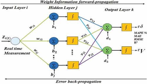
Figure 2 shows the general architecture and working of the MLP algorithm. It contains input time series of different normalized loads demands as actual time series, activation functions, hidden neurons and, learning. The finally error metrics are computed to predicted the difference between actual and predicted load demands.

Figure 2. Multilayer perceptron (MLP) architecture.

Long Short – Term Memory (LSTM)

The architecture of LSTM model is reflected in Figure 3. LSTM is an artificial recurrent neural network (RNN) architecture used in the field of deep learning (Hochreiter, Schmidhuber, and J 1997). LSTM is more robust and appropriate for both short and long term data dependencies. The LSTM was designed to resolve the issues appeared in RNN architecture by adding forget gate, and output gate which manage the vanishing gradient problems very efficiently (Zheng, Yuan, and Chen 2017).

Figure 3. Architecture of LSTM model.

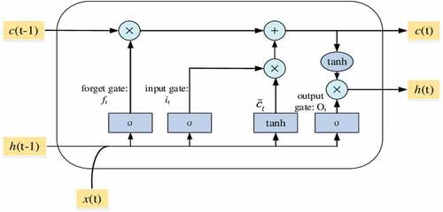
Memory cell of LSTM is considered as its major innovation. To get rid of unnecessary information, the forget gate is used. After that, a sigmoid operation is applied to measure the accelerate the forget state $f_t.$

(2) $f_t=\sigma \left(W_f.\hspace{0.17em}\left[h_{t-1},x_t\right]+b_f\right)\hspace{0.17em}$(2)

The second step is used to know which new data is required to get saved within the cell condition. Another sigmoid layer, known as the “input gate layer,” is used to get the updated information. Then, a $f_t=\sigma \left(W_f.\hspace{0.17em}\left[h_{t-1},x_t\right]+b_f\right)\hspace{0.17em}$ function is used to create a vector $c_t$ of novel values that ought to be updated embarked on upcoming state.

(3) $i_t=\hspace{0.17em}\sigma \left(W_i.\hspace{0.17em}\left[h_{t-1},x_t\right]+b_i\right)$(3)

(4) ${\tilde{c}}_t=tanh\left(W_c.\hspace{0.17em}\left[h_{t-1},x_t\right]+b_c\right)$(4)

In the second step, the old cell state $c_{t-1}$ is refurbished to new cell state $c_t.$ To delete the information from the old cell we can multiply $c_{t-1}$ by $\hspace{0.17em}{f}_t$. Then add $i_t\ast \hspace{0.17em}\underset{t}{c}.$ The new candidate values for updating represented by

(5) $c_t=\hspace{0.17em}{f}_t\ast \hspace{0.17em}{c}_{t-1}+i_t\ast \hspace{0.17em}{\tilde{c}}_t$(5)

In the last step, the output is needed to be decided. The step consists of a couple of further steps: the sigmoid function is used as an output barrier to strain the cell state. Further, the obtained cell state is passed across $\mathrm{t}\mathrm{a}\mathrm{n}\mathrm{h}\left(\cdot \right),\hspace{0.17em}$ the obtained output $o_t$ is multiplied for the calculation of desired information.

(6) $o_t=\hspace{0.17em}\sigma \left(W_o.\hspace{0.17em}\left[h_{t-1},x_t\right]+b_o\right)$(6)

(7) $h_t=\hspace{0.17em}{o}_t\ast tanh\left(c_t\right)\hspace{0.17em}$(7)

We optimized the hyperparameters of LSTM such as Decay rate 0.98, learning rate 0.004, momentum 0.8, batch size 128 to improve the outcomes.

Convolutional Neural Network (CNN)

CNN is also a class of artificial neural networks (ANNs) widely used in many applications such as signal and image processing, computer vision, electricity load forecasting etc. CNN adaptively and automatically learn through backpropagation by utilizing multiple building blocks such as pooling layers, convolution layers, and fully connected layers. CNN is successfully been used in many applications of prediction, recognition, forecasting and objection tracking ranging from healthcare, education, environment, energy, and diverse field of science such as recognition of face (Taigman et al. 2014), object detection & image fragmentation (Shelhamer, Long, and Darrell 2017), video grouping, in-depth assessment as well as image inscribing (Karpathy et al. 2014) classification, day-ahead building-level load forecasts (Cai, Pipattanasomporn, and Rahman 2019), natural language processing (Young et al. 2018), and anomaly detection (Canizo et al. 2019), time series stream forecasting (Zeng, Xiao, and Zhang 2016).

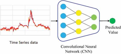
Figure 4 indicates the architecture of the CNN model. A 1D load forecasting time series were used as input to the CNN model, it was processed in different layers of CNN models and finally, the output was in terms of error between actual load demand and predicted values.

Figure 4. CNN architecture for load forecasting.

Performance Evaluation Measures

The quality of predictor was examined by quantitatively measuring the accuracy in term of root mean squared error (RMSE), coefficient of determination (R2), mean square error (MSE) and mean absolute error (MAE), mean absolute percentage error (MAPE). The following renowned error prediction metrics detailed in (Hussain et al. 2019) are used:

1. Root mean squared error (RMSE)

To examine the quality of a predictor, we need a metrics to quantitatively measure its accuracy. In the current study, a quantity called RMSE was introduced for such a purpose, as defined by:

(8) $RMSE=\sqrt{\sum _{i=1}^n{\left(x_i-y_i\right)}^2}\hspace{0.17em}$(8)

Where $x_i$ and $y_i$ denote the measured and predicted values of the i-th sample, and ‘n’ denote the total number of samples of the training dataset. The smaller value of RMSE denote the better set of selected descriptors.

1. Coefficient of determination (R²)

R² can be computed using the following function:

(9) $R^2=\frac{{\sum }_{i=1}^n{\left(x_i-y_i\right)}^2}{{\sum }_{i=1}^n{\left(x_i-\bar{y}\right)}^2}\hspace{0.17em}$(9)

Here $\bar{y}$ denote the average values of all the samples.

1. Mean Square error (MSE)

MSE can be mathematically computed as follow

(10) $MSE=\frac{1}{n}\sum _{i=1}^n{\left(x_i-y_i\right)}^2$(10)

The MSE of an estimator measures the average of the squares of errors or deviations. MSE also denote the second moment of error that incorporate both variance and bias of an estimator.

1. Mean Absolute error (MAE)

MAE is the measure of difference between two consecutive variables, for example variable y and x denote the predicted and observed values, then MAE can be calculated as:

(11) $\mathrm{M}\mathrm{A}\mathrm{E}=\sum _{i=1}^n\frac{\left(y_i-x_i\right)}{n}$(11)

Results

It is calculated as the difference between the real and expected values. If the difference between observed and expected values is small and statistically unbiased, the model best matches the data. The residual plots are frequently used to test the goodness of fitness because they can more easily disclose undesirable residual arrangements that show biased results than numbers. R-squared is an arithmetic metric that demonstrates how well data fits together. Coefficient of determination is another name for it.

Table 1 depicts the load predictions for next 3 months. The LSTM algorithm yielded the highest predictions to forecast ahead 3-month forecasting followed by MLP, CNN + LSTM and CNN by computing the RMSE,R2, MSE, MAE and MAPE error metrics.

Table 1. Prediction of the next 3 months ahead load forecasting.

Method	R2	MAPE	MAE	MSE	RMSE
MLP	0.9803	2.72	327.19	206598.09	454.53
LSTM	0.9808	2.70	325.34	201646.51	449.05
CNN	0.9483	4.76	558.77	543904.56	737.50
CNN+LSTM	0.9673	3.47	416.44	344598.33	587.02

Table 2 depicts the load predictions for next 6 months. To predict the ahead 6 months load forecasting, the MLP followed by LSTM, CNN + LSTM and CNN yielded ahead forecasting performance.

Table 2. Prediction of the next 6 months ahead load forecasting.

Method	R^2	MAPE	MAE	MSE	RMSE
MLP	0.9820	2.36	265.45	140694.59	375.092
LSTM	0.9798	2.58	290.92	158067.24	397.576
N	0.9567	3.83	427.30	338919.63	582.168
CNN+LSTM	0.9720	2.97	330.80	219362.20	468.36

Table 3 depicts the load predictions for next 9 months. LSTM obtained highest prediction when forecasting 9 months ahead followed by MLP, CNN + LSTM and CNN as reflected in the Table

Table 3. Prediction of the next 9 months ahead load forecasting.

Method	R^2	MAPE	MAE	MSE	RMSE
MLP	0.9879	2.38	282.465	146275.23	382.46
LSTM	0.9877	2.37	283.306	148371.15	385.20
CNN	0.9670	3.91	469.927	399613.59	632.15
CNN+LSTM	0.9812	2.87	348.86	227305.65	476.76

Table 4 shows the predicted load forecasting for the next year. As shown in Table 4, the best 1-year prediction output was obtained using LSTM, followed by MLP, CNN + LSTM, and CNN. Figure 5(a) depicts the results of three-month load forecasts produced using four different methods (MLP, LSTM, CNN, and CNN + LSTM). The LSTM is the nearest to the real load curve among the extracted curves, followed by MLP and CNN + LSTM and CNN. As shown in Table 1, the corresponding error values were calculated.

Figure 5. Ahead forecasting using MLP, LSTM, CNN, CNN + LSTM to forecast a) Three months, b) Six months c) Nine months and d) 1 year, e) six years.

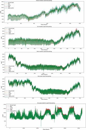
Table 4. Prediction of the next 1 year ahead load forecasting.

Method	R^2	MAPE	MAE	MSE	RMSE
MLP	0.9901	2.30	313.63	179418.40	423.58
LSTM	0.9905	2.25	304.34	172385.71	415.19
CNN	0.9732	3.81	512.08	485420.82	696.72
CNN+LSTM	0.9850	2.75	372.47	271644.37	521.19

Figure 5 (b) depicts the effects of six-month load forecasting using four separate approaches (MLP, LSTM, CNN, and CNN + LSTM). The MLP is the nearest to the real load curve among the extracted curves, followed by LSTM, CNN + LSTM, and CNN. As shown in Table 2, the corresponding error values were obtained. Figure 2 (c) depicts the effects of nine-month load forecasts using four separate approaches (MLP, LSTM, CNN, and CNN + LSTM). The LSTM is the nearest to the real load curve among the extracted curves, followed by MLP, CNN + LSTM, and CNN. As shown in Table 3, the corresponding error values were obtained. Figure 5 (d) depicts the effects of one-year load forecasting using four distinct approaches (MLP, LSTM, CNN, and CNN + LSTM). The LSTM is the nearest to the real load curve among the extracted curves, followed by MLP, CNN + LSTM, and CNN. As shown in Table 4, the corresponding error values were obtained.

The Table and Figure 5 (2) reflect the adhead six years load forecasting. The MLP yielded the highest ahead six years forecasting with R2 (0.9815), MAPE. (2.49), MAE (311.64), RMSE (471.54) followed by LSTM with R2 (0.9619), MAPE (3.03), MAE (416.75), RMSE (677.34); CNN + LSTM with R2 (0.9533), MAPE (3.51), MAE (471.05), RMSE (749.62); and CNN with R2 (0.9283), MAPE (5.42), MAE (673.84), RMSE (928.96).

In the Tables 1–5 and Figure 5, we utilized the machine learning and deep learning models with single and hybrid approach. We aimed to improve the ahead prediction of medium and long-term forecasting from 3 months to six years by optimizing and utilizing hybrid approach. We computed the performance in terms of R-squared error, MAE, MAPE, RMSE, MSE. The minimum difference between actual and predicted model shows the better prediction. Our proposed models with hybrid and parameter optimization approach yielded the improved medium and long-term forecasting.

Table 5. Prediction of ahead six year load forecasting.

Method	R^2	MAPE	MAE	MSE	RMSE
MLP	0.9815	2.49	311.64	222351.94	471.54
LSTM	0.9619	3.03	416.75	458797.66	677.34
CNN	0.9283	5.42	673.84	862976.07	928.96
CNN+LSTM	0.9533	3.51	471.05	561931.59	749.62

Discussions

In this study we predicted the short- and medium-term load forecasting by employing and optimizing the deep learning models. We computed ahead 3, 6, 9 and 12 months forecasting by implemented CNN, LSTM, MLP and CNN + LSTM. The prediction performance was computed with standard performance evaluation metrics. In the literature, The Table 5 reflects the ahead forecasting performance with other machine learning and RNN methods for ahead 3 months prediction. From the results, with previous methods applied such as decision tree (DT), Support Vector Regression (SVR), Auto Regressive Integrated Moving Average (ARIMA), Random Forest (RF), Back Propagation (BP), Recurrent Neural Network (RNN) and date RNN. The highest prediction performance in terms of MAPE was acquired using BP with MAPE (2.85), followed by RNN, DT, gate-RNN, ARIMA, RF and SRV and other performance metrics such as RMSE and MAE accordingly.

In this study, ahead 3 months prediction, we obtained the highest prediction using LSTM with MAPE (2.70) followed by MLP, CNN + LSTM and CNN along with other performance metrics such as RMSE and MAE accordingly as reflected in the Table 5 below.

The results yielded using our approach show that LSTM gives better ahead prediction results to predict ahead 3, 6, 9 and 12-month forecasting.

The Comparison with other studies for 3 months load forecasting is depicted in Table 6. The studies related to hybrid network for the power demand prediction have also been described in Kollia and Kollias (2018) and Tian et al. (2018). In Kollia and Kollias (2018), there has been a transformation of a data set toward the 2-D images by the authors and hence utilized these images functioning as inputs for a CNN-RNN structure. The precision of this CNN-RNN found to be 10% and 26% excessive than ANN and LSTM (Khotanzad, Afkhami-Rohani, and Maratukulam 1998b), individually. Another work depicting about CNN-LSTM constructed hybrid framework has been presented in Tian et al. (2018). According to the study, LSTM as well as CNN work organized horizontally with the characteristics related to input data separately drawn out. Right after the feature extraction by LSTM and CNN, the yields of these two networks have been changed in the consolidated layer from the featured fusion layer.

Table 6. Comparison with other studies for 3 months load forecasting.

Method	RMSE	MAPE (%)	MAE
SVR (Ceperic, Ceperic, and Baric 2013)	1155.91	5.65	979.10
DT (L. Yang and Yang 2019)	701.78	3.02	553.725
ARIMA (Al-Musaylh et al. 2018)	818.07	3.43	628.24
RF (Huo, Shi, and Chang 2016)	943.62	3.48	647.44
BP (L. Yang and Yang 2019)	715.68	2.85	527.99
RNN (L. Yang and Yang 2019)	762.60	2.91	537.40
gate-RNN (L. Yang and Yang 2019)	792.15	3.23	601.51
This approach
MLP	454.53	2.72	327.19
LSTM	449.05	2.70	325.34
CNN	737.50	4.76	558.77
CNN+LSTM	587.02	3.47	416.44

An outfit deep learning strategy utilizing many deep learning systems was depicted in (Qiu et al. 2014). Because the yield may fluctuate when the epoch count is altered, output esteems and for each Deep Belief Network (DBN), values were acquired by using different epochs over a few DBNs in the study. The authors built a deep learning system using the result of a Support Vector Regression (SVR) as input, and it performed 4% and 15% better in estimating power requirements than SVR and DBN, respectively. TS data was prepared using a multi-channel Deep Convolutional Neural Network (DCNN) model in Zheng et al. (2014) and S. Yang et al. (2015), which takes characteristics from a single univariate time series in each channel and aggregates data from complete channels to create an element depiction at the terminal layer. This technique was additionally applied in analyzing pattern data of human behavior along with ECG data.

Conclusion

Since it is used in power grid decision-making and operations, accurate electric load forecasting is important. Accurate electric load forecasting will assist operators in developing an effective business strategy to maximize energy management’s economic benefits. Thus, it is pertinent to develop such load forecasting models which could provide stable, robust and accurate load forecasting. We used a dataset of electric power consumption collected on an hourly basis for this study. We used deep learning models such as LSTM, MLP, CNN + LSTM, and 1D-CNN to forecast the dataset for 3, 6, 9 months, 1 and 6 years ahead. The prediction performance was evaluated in terms of different standard error metrics. Overall, LSTM generated the best ahead load forecasting results, followed by MLP, CNN + LSMT, and CNN. The findings show that the current solution could be more appropriate for potential power expansion issues. As a result, the proposed model is found to outperform benchmark models in terms of forecast results.

Disclosure statement

No potential conflict of interest was reported by the author(s).

Additional information

Funding

The authors extend their appreciation to the Deanship of Scientific Research at King Khalid University for funding this work under grant number (RGP.2/18/43). Princess Nourah bint Abdulrahman University Researchers Supporting Project number (PNURSP2022R237), Princess Nourah bint Abdulrahman University, Riyadh, Saudi Arabia.

References

- Abdulnabi, A. H., G. Wang, J. Lu, and K. Jia. November 2015. Multi-task CNN model for attribute prediction. IEEE Transactions on Multimedia 17(11):1949–2089. doi: 10.1109/TMM.2015.2477680.
- Al-Musaylh, M. S., R. C. Deo, J. F. Adamowski, and Y. Li. 2018. Short-term electricity demand forecasting with mars, svr and arima models using aggregated demand data in Queensland, Australia. Advanced Engineering Informatics 35 (January):1–16. https://linkinghub.elsevier.com/retrieve/pii/S1474034617301477.
- AMJADY, N., and F. KEYNIA. 2009. Short-term load forecasting of power systems by combination of wavelet transform and neuro-evolutionary algorithm. Energy. 34(January):46–57. no. 1. 10.1016/j.energy.2008.09.020.
- Bair, E., T. Hastie, D. Paul, and R. Tibshirani. March 2006. Prediction by supervised principal components. Journal of the American Statistical Association 101(473):119–37. doi: 10.1198/016214505000000628.
- Bengio, Y. 2009. Learning deep architectures for AI. Foundations and Trends® in Machine Learning 2 (1):1–127. http://www.nowpublishers.com/article/Details/MAL-006.
- Bengio, Y. 2013. Deep Learning of Representations: Looking Forward. 7978 LNAI. Lecture Notes in Computer Science (Including Subseries Lecture Notes in Artificial Intelligence and Lecture Notes in Bioinformatics) 1–37.
- Bozchalui, M. C., S. A. Hashmi, H. Hassen, C. A. Canizares, and K. Bhattacharya. December, 2012. Optimal operation of residential energy hubs in smart grids. IEEE Transactions on Smart Grid 3 (4):1755–66. doi:10.1109/TSG.2012.2212032
- Burnham, K. P., and D. R. Anderson, eds. 2004. Model selection and multimodel inference. New York: Springer New York.
- Cai, M., M. Pipattanasomporn, and S. Rahman. 2019. Day-ahead building-level load forecasts using deep learning vs. traditional time-series techniques. Applied Energy 236 (February):1078–88. doi:10.1016/j.apenergy.2018.12.042.
- Canizo, M., I. Triguero, A. Conde, and E. Onieva. 2019. Multi-head CNN–RNN for multi-time series anomaly detection: an industrial case study. Neurocomputing 363 (October):246–60. doi:10.1016/j.neucom.2019.07.034.
- Cao, C., F. Liu, H. Tan, D. Song, W. Shu, W. Li, Y. Zhou, X. Bo, and Z. Xie. 2018. Deep learning and its applications in biomedicine. Genomics, Proteomics & Bioinformatics 16 (1):17–32. doi:10.1016/j.gpb.2017.07.003.
- Ceperic, E., V. Ceperic, and A. Baric. November, 2013. A strategy for short-term load forecasting by support vector regression machines. IEEE Transactions on Power Systems 28 (4):4356–64. doi:10.1109/TPWRS.2013.2269803
- Chan, S. C., K. M. Tsui, H. C. Wu, Y. Hou, Y.-C. Wu, and F. Wu. September 2012. Load/price forecasting and managing demand response for smart grids: methodologies and challenges. IEEE Signal Processing Magazine 29(5):68–85. doi: 10.1109/MSP.2012.2186531.
- Chen, H., D. Ni, J. Qin, S. Li, X. Yang, T. Wang, and P. A. Heng. 2015. Standard plane localization in fetal ultrasound via domain transferred deep neural networks. IEEE Journal of Biomedical and Health Informatics 19 (5):1627–36. doi:10.1109/JBHI.2015.2425041.
- Chen, L.-C., G. Papandreou, I. Kokkinos, K. Murphy, and A. L. Yuille. 2018. DeepLab: semantic image segmentation with deep convolutional nets, atrous convolution, and fully connected CRFs. IEEE Transactions on Pattern Analysis and Machine Intelligence no. 4. 40 (4):834–48. doi:10.1109/TPAMI.2017.2699184.
- Cho, K., and Y. Kim. 2022. Improving streamflow prediction in the WRF-Hydro model with LSTM networks. Journal of Hydrology 605 (February):127297. https://linkinghub.elsevier.com/retrieve/pii/S0022169421013470.
- Ertugrul, Ö. F. 2016. Forecasting electricity load by a novel recurrent extreme learning machines approach. International Journal of Electrical Power & Energy Systems 78 (June):429–35. doi:10.1016/j.ijepes.2015.12.006.
- Fan, G.-F., -L.-L. Peng, and W.-C. Hong. 2018. Short term load forecasting based on phase space reconstruction algorithm and bi-square kernel regression model. Applied Energy. 224(August):13–33. no. 224. 10.1016/j.apenergy.2018.04.075.
- Faria, P., and Z. Vale. August 2011. Demand response in electrical energy supply: an optimal real time pricing approach. Energy 36(8):5374–84. doi: 10.1016/j.energy.2011.06.049.
- Fukushima, K., and S. Miyake. 1982. Neocognitron: A self-organizing neural network model for a mechanism of visual pattern recognition. 267–85.
- Ghahramani, Z. 2004. Unsupervised Learning. 72–112.
- Ghofrani, M., M. Ghayekhloo, A. Arabali, and A. Ghayekhloo. 2015. A hybrid short-term load forecasting with a new input selection framework. Energy no. 81. 81 (March):777–86. doi:10.1016/j.energy.2015.01.028.
- Girshick, R., J. Donahue, T. Darrell, and J. Malik. 2014. Rich feature hierarchies for accurate object detection and semantic segmentation. In 2014 IEEE Conference on Computer Vision and Pattern Recognition, 580–87. IEEE.
- Glorot, X., A. Bordes, and Y. Bengio. 2011. Deep sparse rectifier neural networks. AISTATS ’11: Proceedings of the 14th International Conference on Artificial Intelligence and Statistics 15: 315–23.
- Goodfellow, I., Y. Bengio, and C.A. 2016. Deep Learning.
- Günther, J., P. M. Pilarski, G. Helfrich, H. Shen, and K. Diepold. 2014. First steps towards an intelligent laser welding architecture using deep neural networks and reinforcement learning. Procedia Technology 15:474–83. doi:10.1016/j.protcy.2014.09.007.
- Guo, Y., Y. Liu, A. Oerlemans, S. Lao, S. Wu, Y. G. L.m, Y. Liu, A. Oerlemans, S. Lao, S. Wu, et al. 2016. Deep learning for visual understanding: a review. Neurocomputing no. 187. 187 (April):27–48. doi:10.1016/j.neucom.2015.09.116.
- Gupta, A., M. S. Ayhan, and A. S. Maida. 2013. Natural image bases to represent neuroimaging data. Journal of Machine Learning Research: Workshop and Conference Proceedings 28 (3):977–84.
- Gupta, S., P. Arbeláez, R. Girshick, and J. Malik. 2015. Indoor scene understanding with RGB-D images: bottom-up segmentation, object detection and semantic segmentation. International Journal of Computer Vision 112 (2):133–49. doi:10.1007/s11263-014-0777-6.
- Gupta, S., R. Girshick, P. Arbeláez, and J. Malik. 2014. Learning rich features from RGB-D images for object detection and segmentation. Lecture Notes in Computer Science (Including Subseries Lecture Notes in Artificial Intelligence and Lecture Notes in Bioinformatics) 8695 LNCS (PART 7):345–60.
- Han, L., Y. Peng, Y. Li, B. Yong, Q. Zhou, and L. Shu. 2019. Enhanced deep networks for short-term and medium-term load forecasting. IEEE Access 7:4045–55. doi:10.1109/ACCESS.2018.2888978.
- He, K., X. Zhang, S. Ren, and J. Sun 2016a. Deep residual learning for image recognition. In IEEE Conference on Computer Vision and Pattern Recognition. Vol. 64.
- He, K., X. Zhang, S. Ren, and J. Sun. 2016b. Deep residual learning for image recognition.
- He, Y., Q. Xu, J. Wan, and S. Yang. 2016. Short-term power load probability density forecasting based on quantile regression neural network and triangle kernel function. Energy. 114(November):498–512. no. 114. 10.1016/j.energy.2016.08.023.
- Hinton, G. 2009. Deep belief networks. Scholarpedia 4 (5):5947. http://www.scholarpedia.org/article/Deep_belief_networks.
- Hinton, G., L. Deng, D. Yu, G. E. Dahl, A. Mohamed, N. Jaitly, A. Senior, V. Vanhoucke, P. Nguyen, T. Sainath, et al. 2012. Deep neural networks for acoustic modeling in speech recognition: the shared views of four research groups. IEEE Signal Processing Magazine. 29(6):82–97. doi:10.1109/MSP.2012.2205597.
- Hinton, G. E., S. Osindero, and Y.-W. Teh. July 2006. A Fast Learning Algorithm for Deep Belief Nets. Neural Computation 18(7):1527–54. doi: 10.1162/neco.2006.18.7.1527.
- Hochreiter, S. S., Schmidhuber, and J. J. 1997. Long short-term memory. Neural Computation 9 (8):1735–80. doi:10.1162/neco.1997.9.8.1735.
- Huo, J., T. Shi, and J. Chang. 2016. Comparison of random forest and svm for electrical short-term load forecast with different data sources. In 2016 7th IEEE International Conference on Software Engineering and Service Science (ICSESS), Beijing, China, 1077–80. IEEE. http://ieeexplore.ieee.org/document/7883252/.
- Hussain, L., S. Saeed, A. Idris, I. A. I. A. Awan, S. A. S. A. Shah, A. Majid, B. Ahmed, and Q.-A. Q.-A. Chaudhary. 2019. Regression analysis for detecting epileptic seizure with different feature extracting strategies. Biomedical Engineering/Biomedizinische Technik 64 (6) no. 6December18: 619–42. 10.1515/bmt-2018-0012
- Karpathy, A., and L. Fei-Fei. 2015. Deep visual-semantic alignments for generating image descriptions. In 2015 IEEE Conference on Computer Vision and Pattern Recognition (CVPR), 3128–37. Boston, MA, USA: IEEE.
- Karpathy, A., G. Toderici, S. Shetty, T. Leung, R. Sukthankar, and L. Fei-Fei. 2014. Large-scale video classification with convolutional neural networks. Computer Vision and Pattern Recognition (CVPR), 2014 IEEE Conference On: 1725–32.
- khantach, E., A. M. Hamlich, and N. Eddine Belbounaguia. 2019. Short-term load forecasting using machine learning and periodicity decomposition. AIMS Energy 7 (3):382–94. http://www.aimspress.com/article/10.3934/energy.2019.3.382.
- Khator, S. K., and L. C. Leung. 1997. “Power distribution planning: a review of models and issues. ” {IEEE} {Trans}. {Power} {Syst} no. 3. 12 (3):1151–59. doi:10.1109/59.630455.
- Khotanzad, A., R. Afkhami-Rohani, and D. Maratukulam. 1998a. “ANNSTLF-{artificial} {neural} {network} {short}-{term} {load} {forecaster}- generation three. ” {IEEE} {Trans}. {Power} {Syst} 13(4):1413–22. no. 4. doi:10.1109/59.736285.
- Khotanzad, A., R. Afkhami-Rohani, and D. Maratukulam. 1998b. ANNSTLF-Artificial Neural Network Short-Term Load Forecaster- generation three. IEEE Transactions on Power Systems 13 (4):1413–22. doi:10.1109/59.736285.
- Kollia, I., and S. Kollias. 2018. A deep learning approach for load demand forecasting of power systems. In 2018 IEEE Symposium Series on Computational Intelligence (SSCI), 912–19. IEEE.
- Kong, W., Z. Y. Dong, Y. Jia, D. J. Hill, Y. Xu, and Y. Zhang. 2019. Short-term residential load forecasting based on lstm recurrent neural network. IEEE Transactions on Smart Grid no. 1. 10 (January):841–51. doi:10.1109/TSG.2017.2753802.
- Krizhevsky, A., I. Sutskever, and G. E. Hinton. 2012. Imagenet classification with deep convolutional neural networks. Adv. Neural Inf. Process. Syst 25:1106–14.
- LeCun, Y., and Y. Bengio. 1995. Convolutional networks for images,speech,and time series. Handb. BrainTheoryNeuralNetw.
- LeCun, Y., Y. Bengio, and G. Hinton. 2015. Deep Learning. Nature 521 (7553): 436–44. May 28. 10.1038/nature14539.
- LeCun, Y., P. Haffner, L. Bottou, and Y. Bengio. 1999. Object recognition with gradient-based learning. Springer Berlin Heidelberg 319–45.
- Levi, G., and T. Hassncer. 2015. Age and gender classification using convolutional neural networks. In 2015 IEEE Conference on Computer Vision and Pattern Recognition Workshops (CVPRW), 34–42. IEEE.
- Litjens, G., T. Kooi, B. E. Bejnordi, A. A. A. Setio, F. Ciompi, M. Ghafoorian, J. A. W. M. W. M. van der Laak, B. van Ginneken, and C. I. Sánchez. December, 2017. A survey on deep learning in medical image analysis. Medical Image Analysis 42 (1995):60–88. doi:10.1016/j.media.2017.07.005
- Mamlook, R., O. Badran, and E. Abdulhadi. April, 2009. A fuzzy inference model for short-term load forecasting. Energy Policy 37 (4):1239–48. doi:10.1016/j.enpol.2008.10.051
- Mehmood Butt, F., L. Hussain, A. Mahmood, and K. Javed Lone. 2021. Artificial intelligence based accurately load forecasting system to forecast short and medium-term load demands. Mathematical Biosciences and Engineering 18 (1):400–25. http://www.aimspress.com/article/doi/10.3934/mbe.2021022.
- Metaxiotis, K., A. Kagiannas, D. Askounis, and J. Psarras. June, 2003. Artificial intelligence in short term electric load forecasting: a state-of-the-art survey for the researcher. Energy Conversion and Management 44 (9):1525–34. doi:10.1016/S0196-8904(02)00148-6
- Moslehi, K., and R. Kumar. 2010. A reliability perspective of the smart grid. IEEE Transactions on Smart Grid no. 1. 1 (June):57–64. doi:10.1109/TSG.2010.2046346.
- Murthy Balijepalli, V. S. K., V. Pradhan, S. A. Khaparde, and R. M. Shereef. 2011. Review of demand response under smart grid paradigm. In ISGT2011-India, 236–43. IEEE.
- Oord, A. V. D., S. Dieleman, H. Zen, K. Simonyan, O. Vinyals, A. Graves, N. Kalchbrenner, A. Senior, and K. Kavukcuoglu. 2016. Wavenet: A generative model for raw audio.
- Park, K., S. Yoon, and E. Hwang. 2019. Hybrid load forecasting for mixed-use complex based on the characteristic load decomposition by pilot signals. IEEE Access 7:12297–306. doi:10.1109/ACCESS.2019.2892475.
- Qiu, X., L. Zhang, Y. Ren, P. Suganthan, and G. Amaratunga. 2014. Ensemble deep learning for regression and time series forecasting. In 2014 IEEE Symposium on Computational Intelligence in Ensemble Learning (CIEL), 1–6. IEEE.
- Ranaweera, D. K., N. F. Hubele, and G. G. Karady. May, 1996. Fuzzy Logic for Short Term Load Forecasting. International Journal of Electrical Power & Energy Systems 18 (4):215–22. doi:10.1016/0142-0615(95)00060-7
- Rodrigues Moreno, S., R. Gomes da Silva, V. Cocco Mariani, and L. Dos Santos Coelho. 2020. Multi-step wind speed forecasting based on hybrid multi-stage decomposition model and long short-term memory neural network. Energy Conversion and Management 213 (June):112869. https://linkinghub.elsevier.com/retrieve/pii/S0196890420304076.
- Sermanet, P., D. Eigen, X. Zhang, M. Mathieu, and Y. L. Rob Fergus. 2013. In-Tegrated Recognition. Localization and Detection Using Convolutional Networks 4:16.
- Shelhamer, E., J. Long, and T. Darrell. 2017. Fully convolutional networks for semantic segmentation. IEEE Transactions on Pattern Analysis and Machine Intelligence 39 (4):640–51. doi:10.1109/TPAMI.2016.2572683.
- Shin, H. C., H. R. Roth, M. Gao, L. Lu, Z. Xu, I. Nogues, J. Yao, D. Mollura, and R. M. Summers. 2016. Deep convolutional neural networks for computer-aided detection: CNN architectures, dataset characteristics and transfer learning. IEEE Transactions on Medical Imaging 35 (5):1285–98. doi:10.1109/TMI.2016.2528162.
- Shin, H.-C., L. Lu, and R.m.s 2015. Interleaved text/image deep mining on a large-scale radiology database. Proceedings of the IEEE Conference on Computer Vision and Pattern Recognition. 17: 1090–99.
- Shivarama Krishna, K., and K. Sathish Kumar. 2015. A review on hybrid renewable energy systems. Renewable and Sustainable Energy Reviews 52 (December):907–16. doi:10.1016/j.rser.2015.07.187.
- Singh, P., and P. Dwivedi. 2018. Integration of new evolutionary approach with artificial neural network for solving short term load forecast problem. Applied Energy 217 (May):537–49. doi:10.1016/j.apenergy.2018.02.131.
- Stefenon, S. F., M. H. Dal Molin Ribeiro, A. Nied, V. C. Mariani, L. Dos S. Coelho, D. F. Menegat da Rocha, R. B. Grebogi, and A. E. de B. Ruano. 2020. Wavelet group method of data handling for fault prediction in electrical power insulators. International Journal of Electrical Power & Energy Systems 123 (December):106269. https://linkinghub.elsevier.com/retrieve/pii/S0142061520310711.
- Sundermeyer, M., H. Ney, and R. Schluter. 2015. From feedforward to recurrent LSTM neural networks for language modeling. IEEE/ACM Transactions on Audio, Speech, and Language Processing no. 3. 23 (March):517–29. doi:10.1109/TASLP.2015.2400218.
- Szegedy, C., W. Liu, Y. Jia, P. Sermanet, S. Reed, D. Anguelov, D. Erhan, V. Vanhoucke, and A. Rabinovich 2015. Going deeper with convolutions. C. Szegedy, W. Liu, Y. Jia, P. Sermanet, S. Reed, D. Anguelov, D. Erhan, V. Vanhoucke, and A. Rabinovich. eds. Going Deeper with Convolutions. In Proceedings of the IEEE Conference on Computer Vision and Pattern Recognition, Boston
- Taigman, Y., M. Yang, M. Ranzato, and L. Wolf. 2014. DeepFace: closing the gap to human-level performance in face verification. In Proceedings of the IEEE Computer Society Conference on Computer Vision and Pattern Recognition, 1701–08.
- Taylor, J. W. August 2003. Short-term electricity demand forecasting using double seasonal exponential smoothing. Journal of the Operational Research Society 54(8):799–805. doi: 10.1057/palgrave.jors.2601589.
- Tian, C., J. Ma, C. Zhang, and P. Zhan. 2018. A deep neural network model for short-term load forecast based on long short-term memory network and convolutional neural network. Energies 11 (12): 3493. December 14. 10.3390/en11123493.
- Wen, T. H., M. Gasic, N. Mrksic, P. H. Su, D. Vandyke, and S. Young. 2015. Semantically conditioned LSTM-based natural language generation for spoken dialogue systems. Computer Science > Computation and Language.
- Xie, L., J. Wang, Z. Wei, M. Wang, and Q. Tian. 2016. DisturbLabel: regularizing CNN on the Loss Layer. In 2016 IEEE Conference on Computer Vision and Pattern Recognition (CVPR), 4753–62. IEEE.
- Xu, Y., C. Hu, Q. Wu, S. Jian, Z. Li, Y. Chen, G. Zhang, Z. Zhang, and S. Wang. 2022. Research on particle swarm optimization in lstm neural networks for rainfall-runoff simulation. Journal of Hydrology 608 (May):127553. https://linkinghub.elsevier.com/retrieve/pii/S0022169422001287.
- Yang, J., M. N. Nguyen, P. P. San, X. L. Li, and S. Krishnaswamy 2015a. Deep Convolutional Neural Networks on Multi channel Time Series for Human Activity Recognition. In In Proceedings of the Twenty-Fourth International Joint Conference on Artificial Intelligence.
- Yang, L., and H. Yang. 2019. Analysis of different neural networks and a new architecture for short-term load forecasting. Energies 12 (8): 1433. April 14. 10.3390/en12081433.
- Yang, S., J. Nguyen, M. N. San, P. P. Li, and X. L. Krishnaswamy. 2015b. “Deep convolutional neural networks on {multichannelTimeSeriesforHumanActivityRecognition}. ” in {InProceedingsoftheTwenty}-FourthInternational {JointConferenceonArtificialIntelligence}.
- Young, T., D. Hazarika, S. Poria, and E. Cambria. 2018. Recent trends in deep learning based natural language processing [review article]. IEEE Computational Intelligence Magazine. 13(August):55–75. no. 3. 10.1109/MCI.2018.2840738.
- Yuan, C., S. Liu, and Z. Fang. 2016. Comparison of China’s primary energy consumption forecasting by using arima (the autoregressive integrated moving average) model and GM(1,1) model. Energy 100 (April):384–90. doi:10.1016/j.energy.2016.02.001.
- Zeng, Z., H. Xiao, and X. Zhang. October 2016. Self CNN-based time series stream forecasting. Electronics Letters 52(22):1857–58. doi: 10.1049/el.2016.2626.
- ZHANG, Z., L. GUO, Y. Dai, X. DONG, and P. WANG. 2018. A short-term user load forecasting with missing data. DEStech Transactions on Engineering and Technology Researchno icmeit (June).
- Zheng, H., J. Yuan, and L. Chen. August 2017. Short-term load forecasting using EMD-LSTM neural networks with a xgboost algorithm for feature importance evaluation. Energies 10(8):1168. doi: 10.3390/en10081168.
- Zheng, Y., Q. Liu, E. Chen, Y. Ge, and J. Zhao. 2014. Time series classification using multi-channels deep convolutional neural networks. In International Conference on Web-Age Information Management; Springer: Cham, Switzerland.