Saliency Detection Using a Bio-inspired Spiking Neural Network Driven by Local and Global Saliency

ABSTRACT

The detection of the most salient parts of images as objects in salient object detection tasks mimics human behavior, which is useful for a variety of computer vision applications. In this paper, the Local and Global Saliency Driven Dual-Channel Pulse Coupled Neural Network (LGSD-DCPCNN) model is used to provide a novel strategy for saliency detection. To achieve visually homogeneous sections and save computation costs, the input image is first subjected to superpixel segmentation. The global and local saliency maps are then created using the segmented image’s position, color, and textural properties. The LGSD-DCPCNN network is activated using these saliency maps to extract visually consistent features from the input maps to provide the final saliency map. An extensive qualitative and quantitative performance study is undertaken to assess the efficacy of the proposed method. When compared to state-of-the-art approaches, the experimental results show a considerable improvement in the detection of salient regions. Quantitative analysis of the proposed method reveals a significant improvement in the area under the ROC curve (AUC) score, F-measure score, and mean absolute error (MAE) score. The qualitative analysis describes the proposed algorithm’s ability to detect multiple salient objects accurately while maintaining significant border preservation.

Introduction

Salient object detection techniques mirror human behavior and identify the most prominent regions of images or scenes as an object. It is used in numerous essential applications in the computer vision area. The human visual system (HVS) has an extraordinary capacity to swiftly notice and emphasize the remarkable things or areas in images that are more distinct in appearance and conspicuous. The aim of salient object detection (Shi et al. 2015) is to explore the majority of the distinguishable targets in an image and then fragment it from the rest of the image. Salient object detection, unlike image segmentation tasks, focuses on a small number of intriguing and appealing things. Because of this valuable characteristic, salient object recognition is commonly used as a preliminary step in various applications such as image compression, object recognition, quality assessment, video summarization, image retrieval, object tracking, and image segmentation (Borji et al. 2019; Cong et al. 2018).

Many techniques for recognizing salient objects have emerged in recent years which mainly depend on two approaches to find saliency: bottom-up saliency models and top-down saliency models. Computer vision researchers typically use the bottom-up saliency model to recreate the process of the human gaze. Bottom-up approaches mainly deal with handcrafted low-level features which are generally data-driven. The bottom-up saliency methods use self-information, histogram, regionbased features, locally measured dissimilarities, information contents weighting, and frequency refined approach to compute the saliency (Borji et al. 2019; Cong et al. 2018; Duan et al. 2016; Zhang, Wang, and Lv 2016). Zhang et al. (2017; 2018b) used graph-based approaches to find the saliency which improved the saliency detection results with low-level features, objectness map, and compactness map. (Lu et al. 2019) and (Qi et al. 2015) used multiple graph-based manifold ranking to detect the salient objects. (Wang et al. 2021) used foreground and background seed selection models using graph-based extended random walk model to generate the saliency, in which the background and foreground seeds are produced using the convex hull approach and boundary prior knowledge respectively. All these methods mainly use graph-based saliency models which detects the salient objects by considering color contrast features. So the objects having similar color as background can not be detected by these methods, also textures and edges are not preserved in these methods. Bottom-up approaches are simple to implement and computationally efficient however their performance is limited for low contrast and complicated patterned images. Top-down saliency detection algorithms, on the contrary, are task-driven that are based on task-specific high-level features using convolutional and deep neural networks (Ji et al. 2021). Utilization of such approaches yields improved performance in this area but at the cost of large data availability and substantial computing needs. Also, the results are quantitatively good but lack in preserving the complete boundaries and edges of the objects. As a result, the work of SOD employing handcrafted features plays an important role in today’s world for applications where data availability is limited and low computing complexity is preferred with better preservation of details. There are various machine learning (ML)-based bottom-up saliency detection techniques which have been introduced in recent years. (Pang et al. 2020a) used a bagging-based distributed learning approach for saliency detection which uses the training samples based on the center prior and background prior information. (Lei et al. 2016) uses Bayesian decision framework to refine the primary rough saliency map which is extracted using other existing techniques. (Tong et al. 2015a) employs the bootstrap learning approach to build a powerful classifier that can distinguish between prominent and background objects. The local saliency detection of the proposed method is also based on ML-based bottom-up salient object detection approach.

Many recent approaches (Wang and Peng 2021a; Wang et al. 2021) use saliency map integration to produce the final saliency map. Along with properly detecting saliency, it is very important to fuse different saliency maps to achieve higher performance in a saliency detection task. But a majority of these approaches (Shariatmadar and Faez 2019; Tong et al. 2015a) use simple pixel-wise addition or multiplication of the global and local saliency maps for generating the final saliency maps. Such approaches overlook the intensity variations of the neighboring pixels and may result in edge blurring or artifacts around the object boundaries. Some of the methods also use weighted average-based integration of global and local saliency maps but the selection of weights is mostly done using the hit and trial approach. Meta-heuristic optimization approaches have also been suggested but they suffer from increased computational cost. In context with the above discussion, to overcome the discussed limitations the proposed method uses pulse-coupled neural networks (PCNN)-based saliency map fusion to provide perceptually appealing results. Recently, PCNN-based approaches have also been explored in the area of saliency detection wherein the pixel intensities are used to activate the PCNN neurons (Wang and Shang 2020). These approaches have marked significant performance with improved preservation of object boundaries. Some visual saliency-driven PCNN models have also been presented to achieve image segmentation (Z. Yang, Ma, Lian, Guo et al. 2018) and fusion tasks (Yang and Li 2014). Most of the methods discussed above use the PCNN model to directly generate saliency maps without differentiating between the local and global salient features of the input image while the proposed method uses a dual-channel pulse-coupled network (DCPCNN) (Chai, Li, and Qu 2010) network to fuse the local and global saliency maps by preserving the perceptual quality of an image.

Considering the discussed limitations of the extant work on salient object detection, the proposed method uses pixel-related superpixel segmentation using the Gaussian mixture model which has not been used earlier in a saliency detection task. Also, the combination of various features with center and objectness prior in the generation of global saliency detection is novel in the field of saliency detection. Many graph-related saliency techniques (Yang, Zhang, and Lu 2013; Zhang et al. 2017; Zhang et al., 2018) use only color contrast features to get the saliency map which fails when the contrast between objects and background is same, also these methods can not preserve the boundaries of the objects. The local saliency map generation extracts the K-nearest foreground and background superpixels based on the global saliency map and tries to detect saliency using random forest regression. The novelty of the proposed work as compared to existing saliency detection techniques is both the baseline global saliency map as well as local saliency map use texture-based features that preserves the boundaries of the objects preciously as well as DCPCNN model is first time used in saliency detection task to merge the global and local saliency maps, which helps to preserve the visually prominent features of global and local saliency maps.

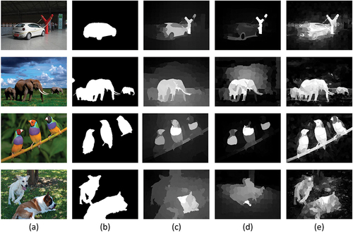
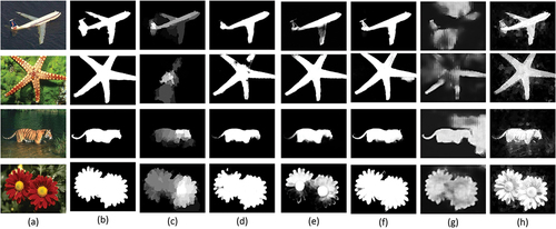
The comparison of the proposed approach with center prior and boundary prior-based saliency detection methods proposed by (Yang, Zhang, and Lu 2013) (GR) and (Yang et al. 2013) (MR), respectively, is shown in Figure 1. Center prior and boundary prior-based methods generally fail to detect the objects away from the image’s center and containing the boundary. While the proposed LGSD-DCPCNN can detect the objects at the center and boundary to a great extent. So the major goal of the proposed work is to consider the image’s local detail with global information to provide boundary preserved and perceptually appealing final saliency maps. Most saliency detection methods take into account only the saliency attributes which are based on the fundamental characteristics of an image, but the overall significance is typically overlooked. The global saliency map represents the global information based on low-level features. It recognizes the entire salient object more precisely with greater integrity. The objectness prior and the center prior used in generating the global saliency maps helps to detect more than one object accurately but is biased as well. On the other hand, the local saliency map takes into account the local spatial variations of an object and helps to detect the salient objects more precisely which are not correctly identified by global saliency maps. So integrating the global and local saliency maps achieves higher performance in saliency detection. In the proposed approach, we use a DCPCNN to process both the source images’ global and local information. The DCPCNN is an extended model of the original PCNN which can process two inputs simultaneously (Chai, Li, and Qu 2010). Processing both the global and local salient features together helps in retaining the most meaningful visual features of the input images and can provide better results. Recently, many researchers are working on video salient object detection (Xu et al. 2019; Xu et al., Jul. 2020) which uses traditional graph-based models to detect salient objects in videos. These methods fail to detect the complete salient objects which can be overcome by extending the proposed work for the video saliency detection task, as the proposed method is computationally efficient.

Figure 1. Comparison with prior based saliency detection methods (a)original image (b)groundtruth (GT) (c)GR (Yang, Zhang, and Lu 2013) (d)MR (Yang et al. 2013) (e)LGSD-DCPCNN.

Taking into account the earlier discussion, in the presented work, the LGSD-DCPCNN model is proposed to merge the image’s local details with global features. The input image is first subjected to superpixel segmentation to obtain visually consistent regions for further processing. Working on a smaller number of superpixels reduces the computational complexity of the proposed approach. Then, global and local saliency maps of the superpixel segmented image are generated and the pixels of the global and local saliency maps are used to activate the neurons of the visual cortex-inspired DCPCNN model. LGSD-DCPCNN model extracts the prominent visual features of the global and local saliency maps and gives a more informative and perceptually appealing resultant saliency maps. The following are the major contributions of the proposed work:

• Unlike current existing saliency map integration models, the novel approach for integrating global and local saliency maps using visual cortex-inspired dual-channel pulse coupled neural network is proposed to generate visually consistent saliency maps from global and local saliency maps with improved boundary preservation.

• To provide computationally efficient performance a pixel-related Gaussian mixture model (GMM) based superpixel segmentation is used as an initial step.

• The global and local saliency maps are produced to provide efficient demarcation between foreground and background regions.

• Detailed experiments on widely known four public datasets demonstrate that the suggested methodology beats the most recent unsupervised handcrafted feature-based algorithms for detecting salient objects in terms of detecting more than one salient object accurately by preserving boundaries and edges of salient objects.

The rest of the paper is structured as follows: Section 2 describes, in brief, the methods and materials used in implementing the proposed salient object detection method. Section 3 outlines in detail the proposed methods’ implementation steps. Section 4 presents the experiments and discussions. The run time of the proposed method is discussed in section 5. Finally, limitations and conclusion are presented in section 6 and section 7, respectively.

Methods and Materials

Superpixel Segmentation

The images’ visual segments are more appealing to HVS than the image pixel values. Superpixels are groupings of pixels that are color and other low-level features alike. A pixel-related GMM enables superpixels to propagate locally throughout an image, reducing computing complexity than earlier expectation maximization (EM) GMM algorithms. In salient object detection tasks, the SLIC superpixel segmentation algorithm is widely used. SLIC is very effective and computationally efficient (Mu, Qi, and Li 2020), also it is excellent at detecting spherical regions but it may not be able to separate items with odd patterns, such as those that are elongated. Pixel-related GMM-based superpixel segmentation (Ban, Liu, and Cao 2018) is also computationally efficient and provides visually consistent superpixels with regular size and can efficiently detect the superpixels with unusual shapes. For a given image $I$ of size $w\times h$, each image pixel is assigned an index $j$. Image pixels are clustered using the GMM superpixel method depending on $w_s$ and $h_s$, that are the superpixel’s allowable width and height, so that $wmod{w}_s$, and $hmod{h}_s$ equal $0$. The number of superpixels, $N$, is computed as in Eq. 1(1) $n_w=\frac{w}{w_s},n_h=\frac{h}{h_s},N=n_w\cdot n_h$(1) and a set of $N$ superpixels, $s{p}_1,s{p}_2,...s{p}_N$, is created.

(1) $n_w=\frac{w}{w_s},n_h=\frac{h}{h_s},N=n_w\cdot n_h$(1)

The label map $L_{b_j}$ for superpixels generation based on pixel-related GMM is given by Eq. 2(2) $L_{b_j}=ar{g}_i\underset{i\in {\mathrm{\Im }}_j}{max}\frac{p(z;{\theta }_i)}{{\sum }_{i\in {\mathrm{\Im }}_j}p(z;{\theta }_i)}$(2) . The superpixels are linked with the Gaussian distribution (Ban, Liu, and Cao 2018), which is defined by the probability distribution function $p(z;{\theta }_i)$ as given in (Ban, Liu, and Cao 2018).

(2) $L_{b_j}=ar{g}_i\underset{i\in {\mathrm{\Im }}_j}{max}\frac{p(z;{\theta }_i)}{{\sum }_{i\in {\mathrm{\Im }}_j}p(z;{\theta }_i)}$(2)

Here, the term ${\mathrm{\Im }}_j$ is a superpixel set belonging to the pixel $j$ which is unique for each $j^{th}$ pixel. Each superpixel $i$ has the local distributing region around it which is called the $i^{th}$ distributing region for superpixel $i$. It usually has a local limitation, which means that each superpixel can only appear in a small area of an image. As a result, the superpixel $i$ must be present in each superpixel set ${\mathrm{\Im }}_j$ in the $i^{th}$ distribution region. The total number of elements in the superpixel set ${\mathrm{\Im }}_j$ is assumed to be constant in this study, which is detailed in (Ban, Liu, and Cao 2018).

Center Prior

The background is more likely to be found toward the image’s edges which has been demonstrated to be true in (Wang and Peng 2021a). Under this concept, a global saliency map is constructed. While capturing the images the objects are mainly placed at the center and saliency is generally considered to be an actual object which takes into account various persons, cars, objects, boxes, etc. Humans observe a scene from the perspective of the intellect, and they tend to focus on the central portions. Cameras are frequently used to capture important items, which are always placed in the image’s central location, which is the center prior. The center is generally formulated using a Gaussian kernel, which was defined as follows:

(3) $Cp=exp\left(-\left(\frac{{\left(X_p-X{ }^{\mathrm{\prime }}\right)}^2}{2{\sigma }_x^2}\right)-\left(\frac{{\left(Y_p-Y{ }^{\mathrm{\prime }}\right)}^2}{2{\sigma }_y^2}\right)\right)$(3)

where $\left(X_p,Y_p\right)$ referred as x and y coordinates of pixel $p$ and $\left(X{ }^{\mathrm{\prime }},Y{ }^{\mathrm{\prime }}\right)$ is center coordinate of an image. ${\sigma }_x^2$ and ${\sigma }_y^2$ are the variance of the image in $x$ and $y$ direction, respectively.

Objectness Prior

Another important consideration is the objectness prior (Alexe, Deselaers, and Ferrari 2012), which is utilized to differentiate the salient object windows from the ones in the background. (Alexe, Deselaers, and Ferrari 2012) present an objectness assessment that combines multiple picture features such as edge density, color contrast, multiscale saliency, and straddles using a Bayesian framework. The approach proposed in (Alexe, Deselaers, and Ferrari 2010) is used to get the objectness information about the region, where the objectness information is given in a window form which indicates whether that particular region contains the salient object or not. As a result, we receive an objectness prior map defined by $Op(m)$ based on how often the pixel $m$ falls into objectness windows. $S_{op}\left(s_i\right)$ is the objectness value calculated as follows:

(4) $S_{op}\left(s_i\right)=\frac{1}{N_{s_i}}\left(\sum _{m\in s_i}Op\left(m\right)\right)$(4)

where $N_{s_i}$ is the total number of pixels in the image region $s_i$.

Random Forest Regression

To tackle regression problems, a Random Forest is an ensemble technique that employs many decision trees and a process known as Bootstrap and Aggregation. Instead of focusing on each decision tree to determine the outcome, the basic idea is to merge the decisions of multiple decision trees. Although every decision tree has significant variance as we mix them all, the total variance is considered to be low since every decision tree has been extensively trained on a sample of data, and so the outcome is based on multiple decision trees rather than just one. In random forest regression, every decision tree is trained with only a few randomly drawn features. And the final output of the random forest regression is the average of the outputs of all the trees. Random forest regression is beneficial for very high-dimensional data. It gives good performance in a salient object detection task.

Dual-channel Pulse Coupled Neural Network

The PCNN model is a bio-inspired spiking neural network that mimics the neuronal assemblies of the mammalian visual cortex. It consists of a single layer, two-dimensional, feed-forward network wherein the neurons are connected latterly (Wang et al. 2016b). Under the impression of an input image, the PCNN neurons respond sharply to various features like position, orientation, direction, etc. Further, the responses of the neurons present within and neighboring cortex columns are also synchronized to generate the final neuronal activity. This feature linking phenomenon generates the coherent spiking of the neurons enabling the PCNN model to extract visually consistent image features. The DCPCNN is an extended model of the original PCNN which can process two inputs simultaneously (Chai, Li, and Qu 2010). The following is the mathematical formulation of a DCPCNN model:

(5) $\left.\begin{array}{c}{E}_{x,y}^1(n)=S_{x,y}^1\\ E_{x,y}^2(n)=S_{x,y}^2\\ L_{x,y}(n)=e^{-{\alpha }_L}{L}_{x,y}(n-1)+V_L\sum _w{W}_{x,y}{Y}_{x,y}(n-1)\\ U_{x,y}^1(n)=E_{x,y}^1(n)(1+{\beta }^1{L}_{x,y}(n))\\ U_{x,y}^2(n)=E_{x,y}^2(n)(1+{\beta }^2{L}_{x,y}(n))\\ U_{x,y}(n)=max\left\{U_{x,y}^1(n),U_{x,y}^2(n)\right\}\\ T_{x,y}(n)=e^{-{\alpha }_T}{T}_{x,y}(n-1)+V_T{Y}_{x,y}(n)\\ Y_{x,y}(n)=\left\{\begin{array}{cc}1,& U_{x,y}(n)>T_{x,y}(n)\\ 0,& otherwise\end{array}\right.\end{array}\right\}$(5)

Here, $E_{x,y}^1$ and $E_{x,y}^2$ denote input feeding channels. $S_{x,y}^1$ and $S_{x,y}^2$ denote the external stimulus to the DCPCNN model which can be either pixel intensities or pixel activities of the input signal. $L_{x,y}$, $U_{x,y}$, $T_{x,y}$, and $Y_{x,y}$ represents the linking input, internal activity, variable threshold, and external activity of neurons, respectively. The surrounding activities of the neurons are weighted by synaptic weight matrix $W_{x,y}$ of window size ($w$). $n$ refers to the number of iterations. ${\alpha }_L$ and ${\alpha }_T$ denote the decay time constants, linking parameters of the two channels are represented by ${\beta }^1$ and ${\beta }^2$. $V_T$ and $V_L$ denote the threshold voltage and linking voltage, respectively. All the free parameters of the DCPCNN model generally depend on the nature of the texture of the image.

Proposed Method

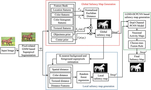
The workflow of the proposed method based on superpixel segmentation and LGSD-DCPCNN is shown in Figure 2. The step-wise implementation information of the proposed method is given below.

Figure 2. Process of proposed algorithm.

Step 1: Superpixel segmentation

In the proposed method the input image is first converted CIELAB color space and segmented to superpixels as indicated in Eq. 6(6) $s{p}_i=[I\left(x,y\right){]}_{L_b==i,wherei\in \left\{1,2,\dots .,N\right\}}$(6) . Here, the number of superpixels $N$ is considered to be 500.

(6) $s{p}_i=[I\left(x,y\right){]}_{L_b==i,wherei\in \left\{1,2,\dots .,N\right\}}$(6)

The labels $L_b$ of the superpixel segmented image are obtained using pixel-related GMM-based superpixel segmentation (Achanta et al. 2012) using Eq. 2(2) $L_{b_j}=ar{g}_i\underset{i\in {\mathrm{\Im }}_j}{max}\frac{p(z;{\theta }_i)}{{\sum }_{i\in {\mathrm{\Im }}_j}p(z;{\theta }_i)}$(2) .

Step 2: Features used for global saliency map generation

In the proposed approach, the global saliency map is constructed using data-driven 81-dimensional low-level features mentioned in Table 1. For every superpixel region $s{p}_i$, the 81-dimensional feature vector is given by $F_{s{p}_i}=\left[f_i^0,f_i^1,\dots ,f_i^{80}\right]$ where $i\in \left\{1,2,\dots ,N\right\}$. The feature vector includes location, color, histogram, and textural features.

Table 1. Features used for generating global saliency map.

Index Component	Feature	Dimension
Features related to Location
0	Normalized x coordinate mean	1
1	Normalized y coordinate mean	1
Features related to color values
2–4	Mean CIELab values	3
5–7	Mean RGB values	3
8	Mean Hue value	1
9	Mean Saturation value	1
Features related to Color Histogram
10	RGB-Histogram	1
11	CIELab-Histogram	1
12	Hue-Histogram	1
13	Saturation-Histogram	1
Features related to Textures
14–21	The Histogram of Gradient	8
22–80	The LBP Histogram	59

Step 3: Center prior used for global saliency map generation

(7) $Cp\left(s{p}_i\right)=exp\left(-\left(\frac{{\left(X-X{ }^{\mathrm{\prime }}\right)}^2}{2{\sigma }_x^2}\right)-\left(\frac{{\left(Y-Y{ }^{\mathrm{\prime }}\right)}^2}{2{\sigma }_y^2}\right)\right)$(7)

where $\left(X,Y\right)$ referred as the average coordinate of the superpixel $s{p}_i$ and $\left(X{ }^{\mathrm{\prime }},Y{ }^{\mathrm{\prime }}\right)$ is center coordinate of an image. ${\sigma }_x^2$ and ${\sigma }_y^2$ are the variance of the image in $x$ and $y$ direction, respectively.

Step 4: Objectness prior used for global saliency map generation

The superpixel region’s average level of objectness is given by Eq. 8(8) $S_{op}\left(s{p}_i\right)=\frac{1}{N_{s{p}_i}}\left(\sum _{m\in s{p}_i}Op\left(m\right)\right)$(8) ,

(8) $S_{op}\left(s{p}_i\right)=\frac{1}{N_{s{p}_i}}\left(\sum _{m\in s{p}_i}Op\left(m\right)\right)$(8)

where $m$ is the pixels contained by $i^{th}$ superpixel and $N_{s{p}_i}$ is the total number of pixel in the $i^{th}$ superpixel.

Step 5: Global saliency map

In the proposed approach, the global contrast of the image regions with the boundary image regions is obtained and the discrepancies between them give the global saliency map. The boundary superpixel regions of an image is denoted by $b_h$ where $h\in \left\{1,2,\dots ,H\right\}$, $H$ is the number of boundary superpixels in that particular image. Using the center prior $Cp\left(s{p}_i\right)$ and objectness prior $S_{op}\left(s{p}_i\right)$, the global saliency map $\left(Sma{p}^G\right)$ is obtained using Eq. 9(9) $Sma{p}^G\left(i\right)=\left(\left(\frac{1}{H}\sum _{h=1}^{H}d\left(F_{s{p}_i},F_{b_h}\right)\right)+S_{op}\left(s{p}_i\right)\right)\cdot Cp\left(s{p}_i\right)$(9) .

(9) $Sma{p}^G\left(i\right)=\left(\left(\frac{1}{H}\sum _{h=1}^{H}d\left(F_{s{p}_i},F_{b_h}\right)\right)+S_{op}\left(s{p}_i\right)\right)\cdot Cp\left(s{p}_i\right)$(9)

Where $d\left(F_{s{p}_i},F_{b_h}\right)$ is the Euclidean distance between the 81-dimensional feature vectors of the $i^{th}$ superpixel region and boundary superpixel regions. Here, we have used Euclidean distance as the feature vector used in the proposed work is not sparse and the Euclidean distance is computationally efficient. Due to non-binary feature data, the Euclidean distance performs better than the $L_1$ distance measure for the proposed work. The $Sma{p}^G$ gives the global saliency map of the superpixel segmented image by considering center prior, objectness prior, and difference of feature vectors of each superpixel to the boundary superpixels of an image. In the proposed method, Eq.9(9) $Sma{p}^G\left(i\right)=\left(\left(\frac{1}{H}\sum _{h=1}^{H}d\left(F_{s{p}_i},F_{b_h}\right)\right)+S_{op}\left(s{p}_i\right)\right)\cdot Cp\left(s{p}_i\right)$(9) gives the global saliency maps by retaining the objects containing the boundary part too to a great extent, even though the boundary prior treats boundary as a background.

Step 6: Features used for generating local saliency map

The local saliency map is constructed using spatial, color, and textural differences of the superpixel with neighboring foreground and background superpixels. In the proposed method global saliency map is considered as the initial saliency map to find the K nearest background as well as K nearest foreground superpixels simply using the nearest Euclidean distance with the superpixel regions of the $2\times mean$ thresholded global saliency map. The features used for local saliency map generation are listed in Table 2. The salient parts which are not recognized in the global saliency map generation method are also recognized by this local saliency-based method using spatial and color contrast features by considering the global saliency map as an initial saliency map. For every $i^{th}$ superpixel $s{p}_i$, firstly we obtain K-nearest foreground superpixels $\left\{s{p}_{f{i}_1},s{p}_{f{i}_2},s{p}_{f{i}_3},......s{p}_{f{i}_K}\right\}$ and K-nearest background superpixels $\left\{s{p}_{b{i}_1},s{p}_{b{i}_2},s{p}_{b{i}_3},......s{p}_{b{i}_K}\right\}$. The value of $K$ is set to 20 as it was giving best F-measure value. The Euclidean distance feature vector of $i^{th}$ superpixel from K-nearest foreground and background superpixels where $\left(d_{fi}\in {\mathbb{R}}^{K\times 1}\right)$ and $\left(d_{bi}\in {\mathbb{R}}^{K\times 1}\right)$ is computed by Eq. 10(10) $d_{fi}=\left[\begin{array}{c}{∥l_i-l_{f{i}_1}∥}_2^2\\ {∥l_i-l_{f{i}_2}∥}_2^2\\ .\\ .\\ .\\ {∥l_i-l_{f{i}_K}∥}_2^2\end{array}\right],d_{bi}=\left[\begin{array}{c}{∥l_i-l_{b{i}_1}∥}_2^2\\ {∥l_i-l_{b{i}_2}∥}_2^2\\ .\\ .\\ .\\ {∥l_i-l_{b{i}_K}∥}_2^2\end{array}\right]$(10) .

(10) $d_{fi}=\left[\begin{array}{c}{∥l_i-l_{f{i}_1}∥}_2^2\\ {∥l_i-l_{f{i}_2}∥}_2^2\\ .\\ .\\ .\\ {∥l_i-l_{f{i}_K}∥}_2^2\end{array}\right],d_{bi}=\left[\begin{array}{c}{∥l_i-l_{b{i}_1}∥}_2^2\\ {∥l_i-l_{b{i}_2}∥}_2^2\\ .\\ .\\ .\\ {∥l_i-l_{b{i}_K}∥}_2^2\end{array}\right]$(10)

Table 2. Features used in local saliency map generation.

Features	Dimension
Superpixels spatial distance from K-nearest foreground superpixels	K
Superpixels spatial distance from K-nearest background superpixels	K
Superpixels color distance from K-nearest foreground superpixels	8 K
Superpixels color distance from K-nearest background superpixels	8 K
Superpixels texture distance from K-nearest foreground superpixels	10 K
Superpixels texture distance from K-nearest background superpixels	10 K

Where $l_i$ indicates the location of the $i^{th}$ superpixel region, $l_{fi}$ and $l_{bi}$ indicates the location of K-nearest foreground and background superpixels, respectively, of the $i^{th}$ superpixel. The color contrast feature vector of $i^{th}$ superpixel region from K-nearest foreground and background superpixels where $\left(d_{c_{fi}}\in {\mathbb{R}}^{8K\times 1}\right)$ and $\left(d_{c_{bi}}\in {\mathbb{R}}^{8K\times 1}\right)$ is computed by Eq. 11(11) $d_{c_{fi}}=\left[\begin{array}{c}d\left(c_i,c_{f{i}_1}\right)\\ d\left(c_i,c_{f{i}_2}\right)\\ .\\ .\\ d\left(c_i,c_{f{i}_K}\right)\end{array}\right],d_{c_{bi}}=\left[\begin{array}{c}d\left(c_i,c_{b{i}_1}\right)\\ d\left(c_i,c_{b{i}_2}\right)\\ .\\ .\\ d\left(c_i,c_{b{i}_K}\right)\end{array}\right]$(11) .

(11) $d_{c_{fi}}=\left[\begin{array}{c}d\left(c_i,c_{f{i}_1}\right)\\ d\left(c_i,c_{f{i}_2}\right)\\ .\\ .\\ d\left(c_i,c_{f{i}_K}\right)\end{array}\right],d_{c_{bi}}=\left[\begin{array}{c}d\left(c_i,c_{b{i}_1}\right)\\ d\left(c_i,c_{b{i}_2}\right)\\ .\\ .\\ d\left(c_i,c_{b{i}_K}\right)\end{array}\right]$(11)

Here, eight color channels i.e. hue, saturation, CIELAB, and RGB are utilized to get the color contrast feature vector. $c_i$, $c_{fi}$ and $c_{bi}$ are 8 dimensional color vectors of the $i^{th}$ superpixel, K-nearest foreground and background superpixels of the $i^{th}$ superpixel, respectively. The distance vectors $d\left(c_i,c_{f{i}_n}\right)$ and $d\left(c_i,c_{b{i}_n}\right)$ indicates the Euclidean distance between $i^{th}$ and $n^{th}$ superpixel color attributes where $n\in \left\{1,2,\dots .,K\right\}$ i.e. K-nearest background and foreground superpixels. The textural distance feature vector of $i^{th}$ superpixel from K-nearest foreground and background superpixels where $\left(d_{t_{fi}}\in {\mathbb{R}}^{10K\times 1}\right)$ and $\left(d_{t_{bi}}\in {\mathbb{R}}^{10K\times 1}\right)$ is computed by Eq. 12(12) $d_{t_{fi}}=\left[\begin{array}{c}d\left(t_i,t_{f{i}_1}\right)\\ d\left(t_i,t_{f{i}_2}\right)\\ .\\ .\\ d\left(t_i,t_{f{i}_K}\right)\end{array}\right],d_{t_{bi}}=\left[\begin{array}{c}d\left(t_i,t_{b{i}_1}\right)\\ d\left(t_i,t_{b{i}_2}\right)\\ .\\ .\\ d\left(t_i,t_{b{i}_K}\right)\end{array}\right]$(12) .

(12) $d_{t_{fi}}=\left[\begin{array}{c}d\left(t_i,t_{f{i}_1}\right)\\ d\left(t_i,t_{f{i}_2}\right)\\ .\\ .\\ d\left(t_i,t_{f{i}_K}\right)\end{array}\right],d_{t_{bi}}=\left[\begin{array}{c}d\left(t_i,t_{b{i}_1}\right)\\ d\left(t_i,t_{b{i}_2}\right)\\ .\\ .\\ d\left(t_i,t_{b{i}_K}\right)\end{array}\right]$(12)

Where $t(\cdot )$ denotes the textural attributes of the superpixels such as gradient mean, gradient direction, and histogram of gradients.

Algorithm 1 Proposed Method

Input: Input image $I(x,y)$ of size $w\times h$

Output: Saliency map $Sma{p}_{x,y}^F$

Parameters: Number of superpixels $(N)$, K nearest background and foreground superpixels $(K)$, DCPCNN parameters: no. of iterations $(n)$, synaptic weight matrix $(W_{x,y})$ of size $w$, decay parameters ${\alpha }_L$ and ${\alpha }_T$, linking parameters of two channels ${\beta }^1$ and ${\beta }^2$, linking voltage $V_T$, threshold voltage $V_T$.

(1) Consider input image as $\mathbf{I}(\mathbf{x}\mathbf{,}\mathbf{y})$. First convert the I(x,y) from RGB to CIELAB color space.

(2) Segment an image into $N$ superpixels given in Eq. 6(6) $s{p}_i=[I\left(x,y\right){]}_{L_b==i,wherei\in \left\{1,2,\dots .,N\right\}}$(6) using label map $L_b$ generated by a pixel related GMM based superpixel segmentation algorithm as in Eq. 2(2) $L_{b_j}=ar{g}_i\underset{i\in {\mathrm{\Im }}_j}{max}\frac{p(z;{\theta }_i)}{{\sum }_{i\in {\mathrm{\Im }}_j}p(z;{\theta }_i)}$(2) .

(3) Obtain the color, spatial distance and texture based 81 dimensional features for global saliency map generation as in Table 1.

(4) Compute the center prior and objectness prior of superpixel segmented image using Eq. 7(7) $Cp\left(s{p}_i\right)=exp\left(-\left(\frac{{\left(X-X{ }^{\mathrm{\prime }}\right)}^2}{2{\sigma }_x^2}\right)-\left(\frac{{\left(Y-Y{ }^{\mathrm{\prime }}\right)}^2}{2{\sigma }_y^2}\right)\right)$(7) and Eq. 8(8) $S_{op}\left(s{p}_i\right)=\frac{1}{N_{s{p}_i}}\left(\sum _{m\in s{p}_i}Op\left(m\right)\right)$(8) , respectively.

(5) Compute the global saliency $Sma{p}_{x,y}^G$ map using difference of 81 dimensional features from boundary superpixels, center prior and objectness prior as per Eq. 9(9) $Sma{p}^G\left(i\right)=\left(\left(\frac{1}{H}\sum _{h=1}^{H}d\left(F_{s{p}_i},F_{b_h}\right)\right)+S_{op}\left(s{p}_i\right)\right)\cdot Cp\left(s{p}_i\right)$(9) .

(6) Considering $Sma{p}_{x,y}^G$ as initial image, obtain K-nearest foreground and background superpixels for each superpixel in an image.

(7) For generating local saliency map, obtain spatial distance, color difference and textural difference features of superpixels from K nearest background and foreground superpixels using Eq. 10(10) $d_{fi}=\left[\begin{array}{c}{∥l_i-l_{f{i}_1}∥}_2^2\\ {∥l_i-l_{f{i}_2}∥}_2^2\\ .\\ .\\ .\\ {∥l_i-l_{f{i}_K}∥}_2^2\end{array}\right],d_{bi}=\left[\begin{array}{c}{∥l_i-l_{b{i}_1}∥}_2^2\\ {∥l_i-l_{b{i}_2}∥}_2^2\\ .\\ .\\ .\\ {∥l_i-l_{b{i}_K}∥}_2^2\end{array}\right]$(10) , Eq. 11(11) $d_{c_{fi}}=\left[\begin{array}{c}d\left(c_i,c_{f{i}_1}\right)\\ d\left(c_i,c_{f{i}_2}\right)\\ .\\ .\\ d\left(c_i,c_{f{i}_K}\right)\end{array}\right],d_{c_{bi}}=\left[\begin{array}{c}d\left(c_i,c_{b{i}_1}\right)\\ d\left(c_i,c_{b{i}_2}\right)\\ .\\ .\\ d\left(c_i,c_{b{i}_K}\right)\end{array}\right]$(11) , and Eq. 12(12) $d_{t_{fi}}=\left[\begin{array}{c}d\left(t_i,t_{f{i}_1}\right)\\ d\left(t_i,t_{f{i}_2}\right)\\ .\\ .\\ d\left(t_i,t_{f{i}_K}\right)\end{array}\right],d_{t_{bi}}=\left[\begin{array}{c}d\left(t_i,t_{b{i}_1}\right)\\ d\left(t_i,t_{b{i}_2}\right)\\ .\\ .\\ d\left(t_i,t_{b{i}_K}\right)\end{array}\right]$(12) , respectively.

(8) Compute the local saliency map $Sma{p}_{x,y}^L$ using random forest regression using features given in Table 2.

(9) Initialize the parameters of DCPCNN.

(10) Feed the two input channels of DCPCNN by pixel intensities of $Sma{p}_{x,y}^G$ and $Sma{p}_{x,y}^L$ and obtain the firing map $Y_{x,y}$ and internal activities $U_{x,y}^1$ and $U_{x,y}^2$ of two channel of DCPCNN using Eq. 13(13) $\left.\begin{array}{c}{E}_{x,y}^1(n)=Sma{p}_{x,y}^L\\ E_{x,y}^2(n)=Sma{p}_{x,y}^G\\ L_{x,y}(n)=e^{-{\alpha }_L}{L}_{x,y}(n-1)+V_L\sum _w{W}_{x,y}{Y}_{x,y}(n-1)\\ U_{x,y}^1(n)=E_{x,y}^1(n)(1+{\beta }^1{L}_{x,y}(n))\\ U_{x,y}^2(n)=E_{x,y}^2(n)(1+{\beta }^2{L}_{x,y}(n))\\ U_{x,y}(n)=max\left\{U_{x,y}^1(n),U_{x,y}^2(n)\right\}\\ T_{x,y}(n)=e^{-{\alpha }_T}{T}_{x,y}(n-1)+V_T{Y}_{x,y}(n)\\ Y_{x,y}(n)=\left\{\begin{array}{cc}1,& U_{x,y}(n)>T_{x,y}(n)\\ 0,& otherwise\end{array}\right.\end{array}\right\}$(13) .

(11) Generate the final saliency map $Sma{p}_{x,y}^F$ based on the choosemax rule to the internal activities $U_{x,y}^1$ and $U_{x,y}^2$ using Eq. 14(14) $Sma{p}_{x,y}^F=\left\{\begin{array}{cc}Sma{p}_{x,y}^L,& U_{x,y}^1(n)>U_{x,y}^2(n)\\ Sma{p}_{x,y}^G,& otherwise\end{array}\right.$(14) .

Step 7: Local saliency map

The local saliency map is obtained using the above mentioned feature vectors by using random forest regression (Breiman 2001) algorithm, as it is very effective for large dimensional feature vectors. For training the random forest, 3000 MSRA-B dataset (Liu et al. 2010) images have been used and annotated ground-truth images are used as labels. For random forest regression, $200$ trees are used and the maximum depth of the tree is considered as $10$ (Becker et al. 2013). The random forest outcome decides whether the superpixel belongs to the background or foreground region and a corresponding saliency map is generated for the particular image. Local saliency map $Sma{p}^L$ is produced using random forest regression, for preserving the local characteristics of the objects that might not get captured by the global saliency map.

Step 8: Global and local saliency map integration using DCPCNN

The $Sma{p}^G$ and $Sma{p}^L$ obtained from step 5 and step 7, respectively, are fed to the two channels of the DCPCNN model shown below:

(13) $\left.\begin{array}{c}{E}_{x,y}^1(n)=Sma{p}_{x,y}^L\\ E_{x,y}^2(n)=Sma{p}_{x,y}^G\\ L_{x,y}(n)=e^{-{\alpha }_L}{L}_{x,y}(n-1)+V_L\sum _w{W}_{x,y}{Y}_{x,y}(n-1)\\ U_{x,y}^1(n)=E_{x,y}^1(n)(1+{\beta }^1{L}_{x,y}(n))\\ U_{x,y}^2(n)=E_{x,y}^2(n)(1+{\beta }^2{L}_{x,y}(n))\\ U_{x,y}(n)=max\left\{U_{x,y}^1(n),U_{x,y}^2(n)\right\}\\ T_{x,y}(n)=e^{-{\alpha }_T}{T}_{x,y}(n-1)+V_T{Y}_{x,y}(n)\\ Y_{x,y}(n)=\left\{\begin{array}{cc}1,& U_{x,y}(n)>T_{x,y}(n)\\ 0,& otherwise\end{array}\right.\end{array}\right\}$(13)

The DCPCNN model used has $w_{dc}=5\times 5$, $n=200$, ${\alpha }_L=1$, ${\alpha }_T=0.2$, ${\beta }^1=3$, ${\beta }^2=3$, $V_L=1$ and $V_T=10$. The internal activities of a neuron for the inputs $E_{x,y}^1$ and $E_{x,y}^2$ are denoted by $U_{x,y}^1$ and $U_{x,y}^2$, respectively. Based on the internal activities of the two channels the final saliency map $Sma{p}_{x,y}^F$ is obtained as follows;

(14) $Sma{p}_{x,y}^F=\left\{\begin{array}{cc}Sma{p}_{x,y}^L,& U_{x,y}^1(n)>U_{x,y}^2(n)\\ Sma{p}_{x,y}^G,& otherwise\end{array}\right.$(14)

Experiments and Discussions

This section presents a detailed qualitative and quantitative performance comparison of the proposed LGSD-DCPCNN method with 17 saliency detection methods. These include methods proposed by Goferman et al. (CA) (Goferman, Zelnik-Manor, and Tal 2011), Yang et al. (GR) (Yang, Zhang, and Lu 2013), Rahtu et al. (SEG) (Rahtu et al. 2010), Yang et al. (MR) (Yang et al. 2013), Jiang et al. (MC) (Jiang et al. 2013), Li et al. (LPS) (Li et al. 2015b), Li et al. (RR) (Li et al. 2015a), Tong et al. (LGF) (Tong et al. 2015b), Zhou et al. (DPSG) (Zhou et al. 2017), Fu et al. (NCUT) (Fu et al. 2015), Yuan et al. (RCRR) (Yuan et al. 2018), Peng et al. (SMD) (Peng et al. 2016), Liu et al. (FCB) (Liu and Yang 2019), Zhang et al. (LSP) (M. Zhang et al., 2018), Pang et al. (BSDL) (Pang et al. 2020b), Wang et al. (CDHL) (Wang and Peng 2021b), and Zang et al. (TMR) (Sun et al. 2022).

Datasets for Salient Object Detection

Four salient object detection datasets mentioned in Table 3 are used for the performance assessment of the proposed method. The datasets contain images with a complex and cluttered background, multiple objects, and low contrast. The performance is evaluated over the entire dataset to show that the proposed LGSD-DCPCNN method is capable of performing consistently and reliably over a diverse set of images.

Table 3. Salient object detection datasets.

Sr. No.	Dataset	No.of images	Description
1	SOD (Movahedi and Elder 2010)	300	Many images include multiple prominent items with little color contrast to the background
2	ECSSD (Shi et al. 2015)	1000	The dataset contains multiple salient objects and also having a complex background, which makes the dataset more challenging for the salient object detection task
3	DUT-OMRON (Yang et al. 2013)	5168	Images of high quality with multiple significant objects, while the backgrounds are relatively cluttered
4	HKU-IS (Li and Yu 2015)	4447	Majority of the images are low contrast with several salient objects

Evaluation Metrics

The proposed method’s performance is assessed using different evaluation measures tabulated in Table 4.

Table 4. Evaluation metrics for salient object detection.

Sr. No.	Evaluation Metrics	Mathematical Expression
1	Precision (Davis and Goadrich 2006)	$Precision=\frac{{\sum }_{x=1}^w{\sum }_{y=1}^{h}Sma{p}_{x,y}^{FT}\cdot G{T}_{x,y}}{{\sum }_{x=1}^w{\sum }_{y=1}^{h}Sma{p}_{x,y}^{FT}}$
2	Recall (Davis and Goadrich 2006)	$Recall=\frac{{\sum }_{x=1}^w{\sum }_{y=1}^{h}Sma{p}_{x,y}^{FT}\cdot G{T}_{x,y}}{{\sum }_{x=1}^w{\sum }_{y=1}^{h}G{T}_{x,y}}$
3	F-measure (Achanta et al. 2009)	$F_m=\frac{(1+{\xi }^2)\cdot Precision\cdot Recall}{({\xi }^2\cdot Precision)+Recall}$ where ${\xi }^2=0.3$
4	MAE (Borji et al. 2015)	$MAE=\frac{1}{w\times h}{\sum }_{x=1}^w{\sum }_{y=1}^h|Sma{p}_{x,y}^{FN}-G{T}_{x,y}|$
5	TPR (Davis and Goadrich 2006)	$TPR=\frac{|Sma{p}^{FT}\cap GT|}{|GT|}$
6	FPR (Davis and Goadrich 2006)	$FPR=\frac{|Sma{p}^{FT}\cap GT|}{|Sma{p}^{FT}\cap GT|+|\bar{S}ma{p}^{FT}\cap \bar{G}T|}$

The evaluation parameters used are the precision-recall (PR) curve, the mean absolute error (MAE) score, F-measure score, receiver operating characteristic (ROC) curve, the area under the ROC curve (AUC) score. F-measure, recall, and precision are used widely for evaluating the overall performance of salient object detection methods (Achanta et al. 2009). In Table 4, $Sma{p}_{x,y}^{FT}$ and $Sma{p}_{x,y}^{FN}$ are thresholded saliency map and normalized saliency map, respectively. $G{T}_{x,y}$ is the groundtruth of the particular image. The F-measure value is the combination of the recall as well as precision values that gives a comprehensive measure for saliency detection tasks. To evaluate these parameters thresholded saliency maps of the obtained gray level saliency maps are needed. To obtain the segmented binary saliency maps, the threshold is altered from 0 to 255 for a saliency map whose grayscale values of the pixels are in the range of [0, 255]. To evaluate the PR curve, the final saliency map $Sma{p}_{x,y}^F$ is binarised using thresholds 0 to 255, and recall and precision values are calculated for each value of threshold which is further used to plot the precision-recall curve. At each threshold, FPR and TPR values are also computed to plot the ROC curve. The ROC curve gives the 2D description of the presented model’s effectiveness, while the AUC value summarizes this description into a single quantity. The area under the ROC curve is used to calculate the AUC value. The true negative assignment of saliency is not taken into account by the overlap-based performance metrics. These metrics prefer approaches that assign strong saliency to prominent pixels while unable to recognize non-salient regions. In some applications like content-aware image resizing the continuous saliency maps have more importance than the thresholded binary saliency maps. In such situations, the MAE gives a comprehensive comparison between the groundtruth and the saliency map. The MAE is computed between the normalized final saliency map $Sma{p}_{x,y}^{FN}$ which is normalized in the range $[0,1]$ and the groundtruth.

Qualitative Analysis

In the qualitative analysis, the saliency maps obtained by the proposed and mentioned other saliency detection methods are evaluated subjectively based on the criteria like, the degree of isolation between foreground and background regions, the region of the salient object to be outlined, homogeneity in highlighting different regions, detection of salient objects in the complex and low contrast background, and detecting more than one salient objects accurately.

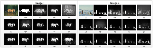
Experimental results are shown in Figure 3–Figure 6 for DUT-OMRON, ECSSD, HKUIS, SOD datasets, respectively. It can be observed from Figure 3 – Figure 6 – Image 1 and Image 2 that CA (Goferman, Zelnik-Manor, and Tal 2011) and SEG (Rahtu et al. 2010) methods are giving blurred results with loss of boundary preservation. Figure 3 – Image 1 and Image 2 of DUT-OMRON dataset indicates that GR (Yang, Zhang, and Lu 2013), MR (Yang et al. 2013), MC (Jiang et al. 2013), RR (Li et al., 2015a), LGF (Tong et al. 2015b), DPSG (Zhou et al. 2017), NCUT (Fu et al. 2015), RCRR (Yuan et al. 2018) and SMD (Peng et al. 2016) methods are able to preserve the boundaries but they are unable to detect all the objects present in an image while the proposed method is able to detect multiple salient objects present in an image accurately with preserving the boundaries. In Figure 4 – Image 1, the proposed method is able to detect the salient objects with preserving the fine details of an image as compared to all other methods except SMD (Peng et al. 2016) method, where the proposed LGSD-DCPCNN and SMD (Peng et al. 2016) give comparable performance. Figure 4 – Image 2 shows the proposed method is accurately detecting the salient object as compared to other methods even the color of the object and background is not so different. From Figure 5 – Image 1, it can be observed that the proposed method detects multiple salient objects with boundary preservation as compared to GR (Yang, Zhang, and Lu 2013), MR (Yang et al. 2013), MC (Jiang et al. 2013), RR (Li et al., 2015a), LGF (Tong et al. 2015b), DPSG (Zhou et al. 2017), NCUT (Fu et al. 2015), RCRR (Yuan et al. 2018) and SMD (Peng et al. 2016) methods. It can be observed that these methods can preserve the boundaries to some extent but fail to detect multiple salient objects. SMD (Peng et al. 2016) method in Figure 5 – Image 2 can detect multiple salient objects but it fails to do so for image shown in Figure 5- Image 1. While the proposed method is detecting multiple salient objects almost for all kinds of images in the HKUIS dataset. Figure 6 – Image 1 shows that the proposed method accurately detects the complete salient object as compared to all the other methods which are miss detecting the tail portion of the object. Figure 6 – Image 2 indicates the image is having 5 salient objects, where only the proposed method can detect all the salient objects accurately compared to all the other methods. From the qualitative analysis, it can be inferred that the proposed LGSD-DCPCNN method outperforms other methods for all the datasets covering different scenarios. In comparison with other saliency methods, LGSD-DCPCNN produces a high-resolution saliency output on a variety of tough natural images. In particular, when comparatively evaluated with other approaches, LGSD-DCPCNN provides a saliency map that evenly highlights salient regions and efficiently suppresses background regions. It effectively separates background and foreground and detects the regions which are salient even in some complex background images. It also detects more than one salient object more accurately than other methods.

Figure 3. Qualitative analysis of the proposed algorithm on DUTOMRON dataset compared to other salient object detection techniques (a)Original Image (b)Groundtruth (c)CA (d)GR (e)SEG (f)MR (g)MC (h)LPS (i)RR (j)LGF (k)DPSG (l)NCUT (m)RCRR (n)SMD (o)LGSD-DCPCNN.

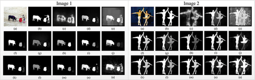
Figure 4. Qualitative analysis of the proposed algorithm on ECSSD dataset compared to other salient object detection techniques (a)Original Image (b)Groundtruth (c)CA (d)GR (e)SEG (f)MR (g)MC (h)LPS (i)RR (j)LGF (k)DPSG (l)NCUT (m)RCRR (n)SMD (o)LGSD-DCPCNN.

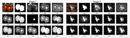
Figure 5. Qualitative analysis of the proposed algorithm on HKUIS dataset compared to other salient object detection techniques (a)Original Image (b)Groundtruth (c)CA (d)GR (e)SEG (f)MR (g)MC (h)LPS (i)RR (j)LGF (k)DPSG (l)NCUT (m)RCRR (n)SMD (o)LGSD-DCPCNN.

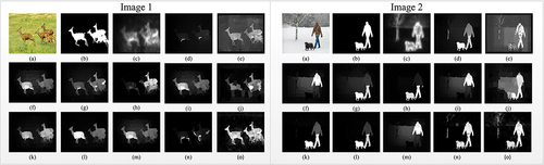
Figure 6. Qualitative analysis of the proposed algorithm on SOD dataset compared to other salient object detection techniques (a)Original Image (b)Groundtruth (c)CA (d)GR (e)SEG (f)MR (g)MC (h)LPS (i)RR (j)LGF (k)DPSG (l)NCUT (m)RCRR (n)SMD (o)LGSD-DCPCNN.

Quantitative Analysis

Quantitative assessment is also carried out to evaluate the proposed LGSD-DCPCNN and other existing techniques. Figures 7 and 8 show comparative results of LGSD-DCPCNN with other saliency detection methods considering the PR curve, and ROC curve, respectively on four benchmark salient object detection datasets mentioned in Table 3. Figure 7 shows that the LGSD-DCPCNN approach gives the comparable or higher performance in terms of PR curve on all the datasets with mentioned salient object detection methods.

Figure 7. Quantitative analysis of the proposed algorithm based on the PR curve on four benchmark saliency detection datasets (a)DUT-OMRON (Yang et al. 2013) (b)ECSSD (Shi et al. 2015) (c)HKUIS (Li and Yu 2015) (d)SOD (Movahedi and Elder 2010).

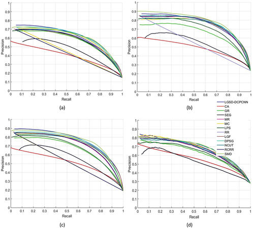
Figure 8. Quantitative analysis of the proposed algorithm based on the ROC curve on four benchmark saliency detection datasets (a)DUT-OMRON (Yang et al. 2013) (b)ECSSD (Shi et al. 2015) (c)HKUIS (Li and Yu 2015) (d)SOD (Movahedi and Elder 2010).

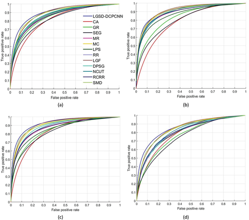
Moreover, the LGSD-DCPCNN method outperforms other methods and gives the best performance for almost all the datasets in terms of ROC curves shown in Figure 8. A comparative analysis based on MAE, F-measure (Fm), and AUC scores is also performed and presented in Table 5. The proposed LGSD-DCPCNN approach achieves the highest AUC score on all the datasets, which demonstrates the superiority of the proposed approach in accurately discriminating the background and foreground areas in salient object detection tasks. Table 5 demonstrate that the LGSD-DCPCNN method also achieves the MAE and Fm values in top-performing methods i.e. at first, second, or the third position as compared to mentioned saliency detection techniques for all the dataset. By comparing the results in Table 5 the following points can be summarized:

• The methods CA (Goferman, Zelnik-Manor, and Tal 2011),SEG (Rahtu et al. 2010), and GR (Yang, Zhang, and Lu 2013) give poor performance as compared to proposed method.

• The proposed method gives the highest AUC score on all the datasets as compared to other mentioned salient object detection techniques.

• On all the datasets, the proposed method gains second or third highest performance in terms of Fm and MAE value as compared to existing salient object detection methods. But the overall performance of the proposed method is better than all the mentioned salient object detection techniques.

• For DUTOMRON dataset: the proposed method gains AUC value $\approx$ 1.46% higher compared to MC (Jiang et al. 2013) and 24.6% higher as compared to BSDL (Pang et al. 2020b) and FCB (Liu and Yang 2019) methods; the proposed method gains Fm value $\approx$ 4.9% higher as compared to TMR (Sun et al. 2022) and 29.38% higher as compared to FCB (Liu and Yang 2019) and MR (Yang et al. 2013) methods; the proposed method achieves MAE value $\approx$ 2.11% lower as compared to BSDL (Pang et al. 2020b) and 31.7% lower as compared to LPS (Li et al., 2015) and MR (C. Yang et al. 2013) methods.

• For HKUIS dataset: the proposed method gains AUC value $\approx$ 0.96% higher compared to MC (Jiang et al. 2013) and 11.57% higher as compared to LPS (Li et al., 2015) method; the proposed method gains Fm value $\approx$ 1.15% higher as compared to DPSG (Zhou et al. 2017) and 35.78% higher as compared to MR (Yang et al. 2013) method; the proposed method achieves MAE value $\approx$ 0.61% lower as compared to DPSG (Zhou et al. 2017) and 12.2% lower as compared to MC (Jiang et al. 2013) method.

• For ECSSD dataset: the proposed method gains AUC value $\approx$ 0.5% higher compared to CDHL (F. Wang and Peng 2021b) and 17.95% higher as compared to FCB (G.H. Liu and Yang 2019) method; the proposed method gains Fm value $\approx$ 0.3% higher as compared to TMR (Sun et al. 2022) and LGF (Tong et al. 2015b) and 22.2% higher as compared to CDHL (F. Wang and Peng 2021b); the proposed method achieves MAE value $\approx$ 1.33% lower as compared to LSP (Zhang et al., 2018) and 34.67% lower as compared to MC (Jiang et al. 2013) method.

• For SOD dataset: the proposed method gains AUC value $\approx$ 0.4% higher compared to MC (Jiang et al. 2013) and 17.47% higher as compared to FCB (Liu and Yang 2019) method; the proposed method gains Fm value $\approx$ 6.56% higher as compared to SMD (Peng et al. 2016) and 25% higher as compared to FCB (Liu and Yang 2019) method; the proposed method achieves MAE value $\approx$ 2.17% lower as compared to SMD (Peng et al. 2016) and 13.48% lower as compared to MC (Jiang et al. 2013) and LPS (Li et al., 2015a) methods.

Table 5. Quantitative analysis of the proposed algorithm with other saliency detection techniques based on the MAE, F-measure (Fm) and AUC values on four benchmark saliency detection datasets. (Red, green, and blue highlight the three leading models, respectively.) MAE less is better, AUC and Fm more is better.

Datasets	DUT-OMRON			HKUIS			ECSSD			SOD
Evaluation metric	AUC	Fmeas	MAE	AUC	Fmeas	MAE	AUC	Fmeas	MAE	AUC	Fmeas	MAE
CA	0.771	0.355	0.254	0.77	0.46	0.274	0.726	0.431	0.309	0.717	0.449	0.313
GR	0.804	0.486	0.259	0.802	0.564	0.256	0.784	0.512	0.283	0.719	0.442	0.318
SEG	0.778	0.394	0.337	0.774	0.464	0.323	0.746	0.394	0.341	0.681	0.316	0.36
MR	0.781	0.48	0.187	0.787	0.517	0.178	0.79	0.691	0.189	0.714	0.57	0.259
MC	0.82	0.533	0.186	0.831	0.678	0.184	0.81	0.699	0.202	0.75	0.59	0.261
LPS	0.767	0.539	0.187	0.752	0.619	0.164	0.782	0.644	0.196	0.703	0.526	0.261
RR	0.782	0.529	0.185	0.796	0.665	0.172	0.796	0.697	0.184	0.713	0.575	0.26
LGF	0.811	0.532	0.178	0.819	0.669	0.177	0.803	0.708	0.196	0.733	0.592	0.256
DPSG	0.796	0.559	0.177	0.808	0.694	0.165	0.795	0.701	0.181	0.71	0.571	0.251
NCUT	0.798	0.568	0.174	0.799	0.679	0.167	0.797	0.69	0.186	0.721	0.577	0.248
RCRR	0.78	0.527	0.182	0.796	0.664	0.171	0.794	0.696	0.184	0.717	0.577	0.257
SMD	0.809	0.538	0.166	0.823	0.691	0.156	0.811	0.729	0.173	0.737	0.61	0.235
FCB	0.668	0.480	0.149	–	–	–	0.702	0.607	0.173	0.641	0.520	0.244
LSP	0.803	0.546	0.133	–	–	–	0.808	0.761	0.152	0.732	0.661	0.226
BSDL	0.668	–	0.145	–	–	–	0.811	–	0.098	0.741	–	0.198
CDHL	0.806	0.709	0.153	–	–	–	0.824	0.581	0.143	–	–	–
TMR	–	0.592	0.159	–	–	–	–	0.708	0.143	–	–	–
LGSD-DCPCNN	0.832	0.621	0.142	0.839	0.702	0.164	0.828	0.71	0.15	0.753	0.65	0.23

Performance Comparison with Deep-Learning-Based Techniques

Furthermore, the proposed method’s overall performance is compared to deep-learning-based techniques which are, KSR (Wang et al. 2016a), RSD-R (Islam, Kalash, and Bruce 2018), PAGR (Zhang et al. 2018c), SSNet (Zeng et al. 2019b), EGNet-R (Zhao et al. 2019), HRSOD-DH (Zeng et al. 2019a), and SCRN (Wu, Su, and Huang 2019). Table 6 gives the comparative analysis of these deep-learning-based techniques with the proposed approach based on MAE and AUC scores. It is evident from Table 6 that the LGSD-DCPCNN-based approach gets equivalent or improved outcomes. It can be inferred clearly from Table 6 that the suggested LGSD-DCPCNN-based approach performs better for the DUT-OMRON, SOD, and HKUIS datasets than most of the deep learning-based approaches. In fact, despite the dataset’s renown for difficult images with dense backgrounds, low contrast images, and images with multiple objects, the proposed method can produce considerably superior results. The proposed approach is capable of detecting objects in images by preserving boundaries in a more efficient manner which is evident from Figure 9 where most of the DL-based techniques fail to produce better qualitative results. Traditional computer vision approaches can typically solve problems faster and with fewer lines of code than deep-learning algorithms (DL), hence DL is often superfluous. Deep neural net (DNN) features are particular to the training dataset and, if poorly created, are unlikely to function well for images other than the training set. On the other hand, traditional computer vision techniques are completely transparent, allowing you to assess whether your idea would perform outside of a training scenario. If anything goes wrong, the parameters can be changed to function properly for a larger range of images. One of the issues in deep learning algorithms is their poor capacity to learn visual relations or determine whether any items in an image are the same or different which is very important in a saliency detection task. The most recent deep learning algorithms may achieve far higher accuracy but at the cost of billions of additional math operations and a higher computing power demand as compared to ML-based bottom-up saliency approaches. So, we can not say that hand-crafted feature-based techniques are obsolete. In the field of computer vision, the integration of handcrafted features and deep features is yielding promising results, which can be considered a future scope of the proposed work.

Table 6. Quantitative analysis of the proposed algorithm with deep learning based saliency detection techniques based on the MAE and AUC values on four benchmark saliency detection datasets. (Bold values show the best outcome, AUC higher is better and MAE lower is better)

Datasets	DUT-OMRON		HKUIS		ECSSD		SOD
Evaluation metric	AUC	MAE	AUC	MAE	AUC	MAE	AUC	MAE
KSR	0.825	0.131	0.824	0.12	0.823	0.134	0.739	0.199
RSD-R	0.812	0.178	0.867	0.155	0.845	0.172	0.753	0.226
PAGR	0.813	0.071	0.867	0.047	0.849	0.061	0.744	0.147
SSNet	0.773	0.056	0.819	0.041	0.813	0.046	0.692	0.118
EGNet-R	–	–	–	–	0.865	0.037	0.782	0.099
HRSOD-DH	0.782	0.065	0.851	0.042	0.839	0.052	0.716	0.139
SCRN	0.864	0.056	0.883	0.034	0.868	0.037	0.781	0.107
LGSD-DCPCNN	0.832	0.142	0.839	0.164	0.828	0.15	0.753	0.23

Figure 9. Qualitative analysis of the proposed algorithm compared to other deep learning based salient object detection techniques (a)Original Image (b)Groundtruth (c)KSR (d)HRSOD-DH (e)PAGR (f)EGNet-R (g)RSD-R (h)LGSD-DCPCNN.

Feature Selection for Global Saliency Map

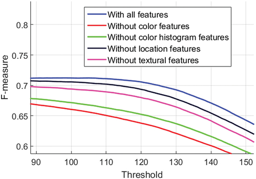
To further understand the significance of each of the four feature attributes i.e. color-based features, color histogram-based features, texture-based features, and location-based features mentioned in Table 1, we constructed four applicable approaches, each deleting one of the features, and compare the results for global saliency map generation in Figure 10. The findings show that every feature category has its own set of favorable conditions that the other three feature categories are unable to address. So, it is important to consider all the features in the global saliency map generation of the proposed work.

Figure 10. Comparative results using F-measure curve on the HKUIS dataset for features selection of global saliency map generation.

Run Time Analysis

This section shows how long the proposed method takes to produce a saliency map. The test is performed on a $300\times 400$ size image on a 64-bit PC with an i7-4770 3.40 GHz processor and 32.0 GB RAM. MATLAB 2017a is used to run all of the routines. Local and global saliency map generation takes 1.23 s and 0.345 s. The time for merging global and local saliency maps using DCPCNN is 0.732 s. Our trained random forest model is 3.8 MB in size, making it a low-weight model which can be considered as efficient to deploy on hardware for any salient object detection application. By adopting a shallow random forest, the size of the trained random forest regression can be further lowered.

Limitations and Future Aspects

The generation of the final saliency map using DCPCNN is mainly dependent on local and global saliency maps. For generating a local saliency map using an ML-based bottom-up saliency approach based, the global saliency map is considered as a baseline map. So, when the global saliency map does not produce good results the proposed method fails to provide the appropriate saliency map as can be seen from Figure 11. For the images in Figure 11, the object and background parts are very difficult to differentiate.

Figure 11. The proposed method’s visual output when baseline saliency maps produce poor results. (a)original image (b)GT (c)global saliency map (d)LGSD-DCPCNN.

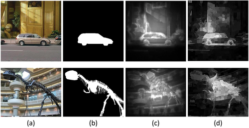
The baseline global saliency map can recognize a few salient objects, but many background disturbances cannot be efficiently eliminated. It is surprising to learn that our proposed LGSD-DCPCNN approach can adequately reflect the contrast between the salient object and the background. Based on the aforementioned observations, we conclude that the LGSD-DCPCNN method performs remarkably even when the baseline saliency map has a poor outcome. Nonetheless, good performance is difficult to achieve when the first saliency map fails to reveal any important saliency information. This difficulty arises in most of the ML-based bottom-up saliency approaches as they require initial knowledge to get the training data. This problem can be tackled using weakly supervised ML-based bottom-up saliency approaches, which may be considered as the future scope of the current work. The discussed limitation can also be overcome using different distance metrics for higher-dimensional data like fractional norms where $L<1$ and by using some feature reduction technique to reduce the dimension of the 81-dimensional feature vector in global saliency map generation which can be considered as the future scope of the proposed work.

Conclusion

This paper presents a novel salient object detection technique that integrates global and local image features using the LGSD-DCPCNN model. A pixel related GMM based superpixel segmentation is employed initially for the input image to speed up the computations. The feature vector of 81 dimensions which contains color, statistical, and texture-based features along with the objectness and center prior, is used to obtain the global saliency maps. While color, spatial, and textural distance features are used to generate the local saliency map using random forest regression which considers the global saliency map as an initial map to find the nearest background and foreground superpixels. The proposed method effectively merges the local and global information taking into account the human visual consistent features of the global and local saliency maps. The use of DCPCNN takes into account the neighborhood pixel variations and helps to preserve the object boundaries without introducing blurring and artifacts. The outcome of substantial experiments carried out on a variety of datasets demonstrates that the suggested combination of global and local saliency maps outperforms other existing saliency detection methods in terms of AUC, F-measure, and MAE scores as well as it gives a comparable performance with many of the deep learning techniques. The proposed method for detecting salient objects proves its superiority in detecting multiple salient objects by preserving the fine details and boundaries of the objects which is evident from the qualitative analysis of the proposed algorithm.

Disclosure Statement

No potential conflict of interest was reported by the author(s).

Additional information

Funding

The authors have no funding to report.

References

- Achanta, R., S. Hemami, F. Estrada, and S. Susstrunk (2009). Frequency-tuned salient region detection. In 2009 ieee conference on computer vision and pattern recognition, Miami, Florida (pp. 1597–2928).
- Achanta, R., A. Shaji, K. Smith, A. Lucchi, P. Fua, and S. Süsstrunk. 2012. Slic superpixels compared to state-of-the-art superpixel methods. IEEE Transactions on Pattern Analysis and Machine Intelligence 34 (11):2274–82. doi:10.1109/TPAMI.2012.120.
- Alexe, B., T. Deselaers, and V. Ferrari (2010). What is an object? In 2010 ieee computer society conference on computer vision and pattern recognition, San Francisco, CA (pp. 73–80).
- Alexe, B., T. Deselaers, and V. Ferrari. 2012. Measuring the objectness of image windows. IEEE Transactions on Pattern Analysis and Machine Intelligence 34 (11):2189–202. doi:10.1109/TPAMI.2012.28.
- Ban, Z., J. Liu, and L. Cao. 2018. Superpixel segmentation using Gaussian mixture model. IEEE Transactions on Image Processing 27 (8):4105–17. doi:10.1109/TIP.2018.2836306.
- Becker, C., R. Rigamonti, V. Lepetit, and P. Fua (2013, September). Supervised feature learning for curvilinear structure segmentation. In International conference on medical image computing and computer-assisted intervention, Nagoya, Japan (pp. 526–33).
- Borji, A., M.-M. Cheng, H. Jiang, and J. Li. 2015. Salient object detection: A benchmark. IEEE Transactions on Image Processing 24 (12):5706–22. doi:10.1109/TIP.2015.2487833.
- Borji, A., M.-M. Cheng, Q. Hou, H. Jiang, and J. Li. 2019. Salient object detection: A survey. Computational Visual Media 5 (2):117–50. doi:10.1007/s41095-019-0149-9.
- Breiman, L. 2001. Random forests. Machine Learning 45 (1):5–32. doi:10.1023/A:1010933404324.
- Chai, Y., H. Li, and J. Qu. 2010. Image fusion scheme using a novel dual-channel pcnn in lifting stationary wavelet domain. Optics Communications 283 (19):3591–602. doi:10.1016/j.optcom.2010.04.100.
- Cong, R., J. Lei, H. Fu, M.-M. Cheng, W. Lin, and Q. Huang. 2018. Review of visual saliency detection with comprehensive information. IEEE Transactions on Circuits and Systems for Video Technology 29 (10):2941–59. doi:10.1109/TCSVT.2018.2870832.
- Davis, J., and M. Goadrich (2006). The relationship between precision-recall and roc curves. In Proceedings of the 23rd international conference on machine learning, Pittsburgh Pennsylvania, USA (pp. 233–40).
- Duan, Q., T. Akram, P. Duan, and X. Wang. 2016. Visual saliency detection using information contents weighting. Optik 127 (19):7418–30. doi:10.1016/j.ijleo.2016.05.027.
- Fu, K., C. Gong, I. Y.-H. Gu, and J. Yang. 2015. Normalized cut-based saliency detection by adaptive multi-level region merging. IEEE Transactions on Image Processing 24 (12):5671–83. doi:10.1109/TIP.2015.2485782.
- Goferman, S., L. Zelnik-Manor, and A. Tal. 2011. Context-aware saliency detection. IEEE Transactions on Pattern Analysis and Machine Intelligence 34 (10):1915–26. doi:10.1109/TPAMI.2011.272.
- Guo, Y., Z. Yang, Y. Ma, J. Lian, and L. Zhu, et al. 2018. Saliency motivated improved simplified pcnn model for object segmentation. Neurocomputing 275:2179–90. doi:10.1016/j.neucom.2017.10.057.
- Islam, M. A., M. Kalash, and N. D. Bruce (2018). Revisiting salient object detection: Simultaneous detection, ranking, and subitizing of multiple salient objects. In Proceedings of the ieee conference on computer vision and pattern recognition, Salt Lake City, UT, USA (pp. 7142–50).
- Ji, Y., H. Zhang, Z. Zhang, and M. Liu. 2021. Cnn-based encoder-decoder networks for salient object detection: A comprehensive review and recent advances. Information Sciences 546:835–57. doi:10.1016/j.ins.2020.09.003.
- Jiang, B., L. Zhang, H. Lu, C. Yang, and M.-H. Yang (2013). Saliency detection via absorbing markov chain. In Proceedings of the ieee international conference on computer vision, Sydney, Australia (pp. 1665–72).
- Lei, J., B. Wang, Y. Fang, W. Lin, P. Le Callet, N. Ling, and C. Hou. 2016. A universal framework for salient object detection. IEEE Transactions on Multimedia 18 (9):1783–95. doi:10.1109/TMM.2016.2592325.
- Li, G., and Y. Yu (2015). Visual saliency based on multiscale deep features. In Proceedings of the ieee conference on computer vision and pattern recognition, Boston, MA, USA (pp. 5455–63).
- Li, C., Y. Yuan, W. Cai, Y. Xia, and D. Dagan Feng (2015a). Robust saliency detection via regularized random walks ranking. In Proceedings of the ieee conference on computer vision and pattern recognition, Boston, MA, USA (pp. 2710–17).
- Li, H., H. Lu, Z. Lin, X. Shen, and B. Price. 2015b. Inner and inter label propagation: Salient object detection in the wild. IEEE Transactions on Image Processing 24 (10):3176–86. doi:10.1109/TIP.2015.2440174.
- Liu, T., Z. Yuan, J. Sun, J. Wang, N. Zheng, X. Tang, and H.-Y. Shum. 2010. Learning to detect a salient object. IEEE Transactions on Pattern Analysis and Machine Intelligence 33 (2):353–67.
- Liu, G.-H., and J.-Y. Yang. 2019. Exploiting color volume and color difference for salient region detection. IEEE Transactions on Image Processing 28 (1):6–16. doi:10.1109/TIP.2018.2847422.
- Lu, Y., K. Zhou, X. Wu, and P. Gong. 2019. A novel multi-graph framework for salient object detection. The Visual Computer 35 (11):1683–99. doi:10.1007/s00371-019-01637-2.
- Movahedi, V., and J. H. Elder (2010). Design and perceptual validation of performance measures for salient object segmentation. In 2010 ieee computer society conference on computer vision and pattern recognition-workshop, San Francisco, CAs (pp. 49–56).
- Mu, X., H. Qi, and X. Li. 2020. Automatic segmentation of images with superpixel similarity combined with deep learning. Circuits, Systems, and Signal Processing 39 (2):884–99. doi:10.1007/s00034-019-01249-0.
- Pang, Y., X. Yu, Y. Wu, C. Wu, and Y. Jiang. 2020a. Bagging-based saliency distribution learning for visual saliency detection. Signal Processing: Image Communication 87:115928.
- Pang, Y., X. Yu, Y. Wu, C. Wu, and Y. Jiang. 2020b. Bagging-based saliency distribution learning for visual saliency detection. Signal Processing: Image Communication 87:115928.
- Peng, H., B. Li, H. Ling, W. Hu, W. Xiong, and S. J. Maybank. 2016. Salient object detection via structured matrix decomposition. IEEE Transactions on Pattern Analysis and Machine Intelligence 39 (4):818–32. doi:10.1109/TPAMI.2016.2562626.
- Qi, W., -M.-M. Cheng, A. Borji, H. Lu, and L.-F. Bai. 2015. Saliencyrank: Two-stage manifold ranking for salient object detection. Computational Visual Media 1 (4):309–20. doi:10.1007/s41095-015-0028-y.
- Rahtu, E., J. Kannala, M. Salo, and J. Heikkilä (2010). Segmenting salient objects from images and videos. In European conference on computer vision, Heraklion, Crete, Greece (pp. 366–79).
- Shariatmadar, Z. S., and K. Faez. 2019. Visual saliency detection via integrating bottom-up and top-down information. Optik 178:1195–207. doi:10.1016/j.ijleo.2018.10.096.
- Shi, J., Q. Yan, L. Xu, and J. Jia. 2015. Hierarchical image saliency detection on extended cssd. IEEE Transactions on Pattern Analysis and Machine Intelligence 38 (4):717–29. doi:10.1109/TPAMI.2015.2465960.
- Sun, X., X. Zhang, C. Xu, M. Xiao, and Y. Tang. 2022. Tensorial multiview representation for saliency detection via nonconvex approach. IEEE Transactions on Cybernetics 1–14. doi:10.1109/TCYB.2021.3139037.
- Tong, N., H. Lu, X. Ruan, and M.-H. Yang (2015a). Salient object detection via bootstrap learning. In Proceedings of the ieee conference on computer vision and pattern recognition, Boston, MA, USA (pp. 1884–92).
- Tong, N., H. Lu, Y. Zhang, and X. Ruan. 2015b. Salient object detection via global and local cues. Pattern Recognition 48 (10):3258–67. doi:10.1016/j.patcog.2014.12.005.
- Wang, T., L. Zhang, H. Lu, C. Sun, and J. Qi (2016a). Kernelized subspace ranking for saliency detection. In European conference on computer vision, Amsterdam, The Netherlands (pp. 450–66).
- Wang, Z., S. Wang, Y. Zhu, and Y. Ma. 2016b. Review of image fusion based on pulse-coupled neural network. Archives of Computational Methods in Engineering 23 (4):659–71. doi:10.1007/s11831-015-9154-z.
- Wang, M., and X. Shang. 2020. An improved simplified pcnn model for salient region detection. The Visual Computer 38 1–13.
- Wang, H., C. Zhu, J. Shen, Z. Zhang, and X. Shi. 2021. Salient object detection by robust foreground and background seed selection. Computers & Electrical Engineering 90:106993. doi:10.1016/j.compeleceng.2021.106993.
- Wang, F., and G. Peng. 2021a. Saliency detection based on color descriptor and high-level prior. Machine Vision and Applications 32 (6):1–12. doi:10.1007/s00138-021-01250-1.
- Wang, F., and G. Peng. 2021b. Saliency detection based on color descriptor and high-level prior. Machine Vision and Applications 32 1–12.
- Wu, Z., L. Su, and Q. Huang (2019). Stacked cross refinement network for edge-aware salient object detection. In Proceedings of the ieee/cvf international conference on computer vision, Seoul, Korea (South) (pp. 7264–73).
- Xu, M., B. Liu, P. Fu, J. Li, and Y. H. Hu. 2019. Video saliency detection via graph clustering with motion energy and spatiotemporal objectness. IEEE Transactions on Multimedia 21 (11):2790–805. doi:10.1109/TMM.2019.2914889.
- Xu, M., B. Liu, P. Fu, J. Li, Y. H. Hu, and S. Feng. July 2020. Video salient object detection via robust seeds extraction and multi-graphs manifold propagation. IEEE Transactions on Circuits and Systems for Video Technology 30(7):2191–206.
- Yang, C., L. Zhang, and H. Lu. 2013. Graph-regularized saliency detection with convex-hull- based center prior. IEEE Signal Processing Letters 20 (7):637–40. doi:10.1109/LSP.2013.2260737.
- Yang, C., L. Zhang, H. Lu, X. Ruan, and M.-H. Yang (2013). Saliency detection via graph- based manifold ranking. In Proceedings of the ieee conference on computer vision and pattern recognition, Portland, OR, USA (pp. 3166–73).
- Yang, B., and S. Li. 2014. Visual attention guided image fusion with sparse representation. Optik 125 (17):4881–88. doi:10.1016/j.ijleo.2014.04.036.
- Yuan, Y., C. Li, J. Kim, W. Cai, and D. D. Feng. 2018. Reversion correction and regularized random walk ranking for saliency detection. IEEE Transactions on Image Processing 27 (3):1311–22. doi:10.1109/TIP.2017.2762422.
- Zeng, Y., P. Zhang, J. Zhang, Z. Lin, and H. Lu (2019a). Towards high-resolution salient object detection. In Proceedings of the ieee/cvf international conference on computer vision, Seoul, Korea (South) (pp. 7234–43).
- Zeng, Y., Y. Zhuge, H. Lu, and L. Zhang (2019b). Joint learning of saliency detection and weakly supervised semantic segmentation. In Proceedings of the ieee/cvf international conference on computer vision, Seoul, Korea (South) (pp. 7223–33).
- Zhang, -Y.-Y., Z.-P. Wang, and X.-D. Lv. 2016. Saliency detection via sparse reconstruction errors of covariance descriptors on riemannian manifolds. Circuits, Systems, and Signal Processing 35 (12):4372–89. doi:10.1007/s00034-016-0267-x.
- Zhang, L., J. Ai, B. Jiang, H. Lu, and X. Li. 2017. Saliency detection via absorbing markov chain with learnt transition probability. IEEE Transactions on Image Processing 27 (2):987–98. doi:10.1109/TIP.2017.2766787.
- Zhang, M., Y. Pang, Y. Wu, Y. Du, H. Sun, and K. Zhang. 2018a. Saliency detection via local structure propagation. Journal of Visual Communication and Image Representation 52:131–42. doi:10.1016/j.jvcir.2018.01.004.
- Zhang, Q., J. Lin, W. Li, Y. Shi, and G. Cao. 2018b. Salient object detection via compactness and objectness cues. The Visual Computer 34 (4):473–89. doi:10.1007/s00371-017-1354-0.
- Zhang, X., T. Wang, J. Qi, H. Lu, and G. Wang (2018c). Progressive attention guided recurrent network for salient object detection. In Proceedings of the ieee conference on computer vision and pattern recognition, Salt Lake City, UT, USA (pp. 714–22).
- Zhao, J.-X., -J.-J. Liu, D.-P. Fan, Y. Cao, J. Yang, and -M.-M. Cheng (2019). Egnet: Edge guidance network for salient object detection. In Proceedings of the ieee/cvf international conference on computer vision, Seoul, Korea (South) (pp. 8779–88).
- Zhou, L., Z. Yang, Z. Zhou, and D. Hu. 2017. Salient region detection using diffusion process on a two-layer sparse graph. IEEE Transactions on Image Processing 26 (12):5882–94. doi:10.1109/TIP.2017.2738839.