Stock Market Prediction of NIFTY 50 Index Applying Machine Learning Techniques

ABSTRACT

The stock market is viewed as an unpredictable, volatile, and competitive market. The prediction of stock prices has been a challenging task for many years. In fact, many analysts are highly interested in the research area of stock price prediction. Various forecasting methods can be categorized into linear and non-linear algorithms. In this paper, we offer an overview of the use of deep learning networks for the Indian National Stock Exchange time series analysis and prediction. The networks used are Recurrent Neural Network, Long Short-Term Memory Network, and Convolutional Neural Network to predict future trends of NIFTY 50 stock prices. Comparative analysis is done using different evaluation metrics. These analysis led us to identify the impact of feature selection process and hyper-parameter optimization on prediction quality and metrics used in the prediction of stock market performance and prices. The performance of the models was quantified using MSE metric. These errors in the LSTM model are found to be lower compared to RNN and CNN models.

Introduction

Stock market trading has gained enormous popularity globally and for many people, it is a part of the everyday routine to make gains. But forecasting the movement of stock prices is a challenge due to the complexity of stock market data. Forecasting can be defined as the prediction of some future events by analyzing the historical data. It spans many areas including industry, business, economics, and finance. However, as the technology is advancing, there is an improvement in the opportunity to gain a steady fortune from the stock market and it also helps experts find the most useful indicators to make much better forecasting. Many of the forecasting problems involve the analysis of time. Time-series data analysis helps to recognize patterns, trends and phases or cycles that are present in the data. In the case of the stock market, early knowledge of bullish or bearish mode serves to wisely invest capital. The study of trends also helps to recognize the best-performing companies over a given period. This makes analysis and forecasting of the time series a significant research field. Deep learning is a framework for training and modeling neural networks that in many learning tasks, especially image and voice recognition, have recently exceeded all traditional methods. The paper that we have presented modeled and predicted the stock prices of NIFTY 50 index which is a diversified index of 50 stocks covering 12 Indian economy sectors listed in the Indian National Stock Exchanges (NSE). We selected the NSE because it holds a place of prominence globally and it stands among the highest in innovation and technical development. Furthermore, we focus on three different architectures that are RNN, LSTM, and CNN to predict future trends of stock prices as well as the financial time series based on historical data. The following section will introduce some of the works that have been carried out by researchers in adopting and applying different techniques and models in the prediction of the stock market price as well as the architecture of the suggested prediction models used in this research. The third section presents the proposed methodology that consists of several stages. The experimental results of the simulations on NIFTY 50 data will be analyzed and discussed in the fourth section. Finally, the fifth section includes the conclusion and describing the future work of the research.

Research Objectives

Many researchers and investors are interested in the finance market. Thus, they need guidance and reliable predictions to invest wisely. Recently, stock market forecasting has gained more interest because investors may be better informed if the market path is accurately predicted. Many businesses already use the concept of deep learning and machine learning to make profits. Investment and trading profitability in the stock market is largely dependent on predictability. If any system that can reliably predict the volatile stock market movements was created, the system’s owner would become wealthy. More about the expected market trends will help market regulators to take corrective measures.

We tried to gain insight into market behavior over time with an effective stock prediction model. The main objectives of the research are as follows: 1. To identify the impact of feature selection process and hyper-parameter optimization on prediction quality and metrics used in the prediction of stock market performance and prices. 2. To analyze historical data of NIFTY 50 and used it for training and validation purposes. 3. The use deep learning models to forecast the Price of NIFTY 50 index. 4. To examine the results and analyze the efficiency of each model evaluation metrics, features and epochs.

Those objectives investigate the best forecasting models. Thus, providing a comprehensive analysis of the NIFTY 50 index.

Literature Review

Despite the increase in stock market prediction techniques, some analysts and scholars believe that the stock market is unpredictable. According to the authors in (Fama 1995) and (Malkiel 2005), the stock market is stochastic and is therefore not predictable. This leads to the two well-known theories, the efficient market hypothesis (EMH) and the random-walk hypothesis (RWH). EMH is one of the popular theories in financial economics. Fama hypothesized that the stock market is “informationally efficient.” The reliability of this theory is difficult because the hypothesizer Fama revised it and graded it in three stages of effectiveness as weak, semistrong and the strong form (Fama 1970). On the other hand, the RWH holds the belief that the stock price is essentially stochastic; thus, any attempt or effort to predict the future stock price will ultimately fail (Alkhoshi and Saeid 2018). Nevertheless, the EMH is vulnerable to debate about which one, if any, is closely testing these two theories, since one has fundamental and technical knowledge about the equity market, there is new issue to forecast the stock market. Through understanding and knowledge of a firm’s historical stock data and fundamental or technical data, we can contribute to a reliable forecast of the company’s future stock price. The study of (Dahir et al. 2018) explores the dynamic relationships between exchange rates and stock returns in Brazil, Russia, India, China, and South Africa (BRICS) using wavelet analysis. The findings show that in the medium and long term, there is a high correlation between exchange rates and stock returns, indicating that exchange rates in Brazil and Russia lead stock returns. Also, these findings have significant consequences for investors in frequency-varying exchange rates and stock returns, as well as regulators who should consider developing appropriate regulatory measures to avoid financial risk. Researchers in (Aziz and Ahmad 2018) examined the link between minimum daily returns and future monthly returns during the period (1999–2014) in India’s emerging stock market. The findings show that stocks with higher minimum daily returns in 1 month offer larger returns in the following month. They also demonstrate that the relationship between minimum daily returns and future stock returns is dynamic and quantile dependent by using quantile regression. By analyzing the historical data, forecasts can be described as predictions of any future events. Many of the issues of forecasting include time analysis. Time-series data analysis helps to recognize patterns, trends and phases or cycles that are present in the data. The early understanding of bullish or bearish mode helps to spend capital wisely in the case of the stock market. The pattern analysis also helps to classify the highest performing companies over a given period of time. This makes analysis and forecasting of time series an important research area. The existing stock price forecasting approaches can be listed as follows:

1. Fundamental Analysis and Technical Analysis

2. Machine Learning Models

3. Neural Network Models

Fundamental and Technical Analysis

The stock market’s movements are analyzed and predicted using fundamental and technical analysis. The fundamental analysis includes an in-depth analysis of the performance of a company. This method is ideally suited for forecasting for the long term (As 2013). Moreover, it has been occasionally proved to be a strong indicator of the movement of stock prices in the works of (Checkley, Higón, and Alles 2017, Tsai and Wang 2017) and (Zhang et al. 2018). Whereas, technical analysis is a method of assessing stocks by examining market behavior, past prices and volume produced statistics. It’s looking peaks, bottoms, trends, and other factors that influence the price movement of a stock. This method supports short-term forecasts (Drakopoulou 2016). The following research forecast the future movement of stock-prices based on technical analysis (Putriningtiyas and Mochammad 2017, Nti, Felix, and Asubam 2020). Both these methods are having their limitations and fail to give expected results. Moreover, the results produced by these tools can be interpreted by the experts only and also these tools require a lot of time in a modern dynamic trading environment.

Machine Learning Models

Machine learning is a field of Artificial Intelligence (AI). It has been widely studied and explored for the prediction of stock price direction. Machine learning tasks are usually classified as supervised and unsupervised learning. Supervised learning techniques are used to collect training data in which instances are marked with labels and each label shows a specific instance’s class (Ashfaq et al. 2017). Supervised learning techniques like Linear Regression, Support Vector Machine (SVM), Random Forest, Nearest Neighbor, and Decision Trees can attempt to forecast historical data-based stock market prices and patterns as well as provide useful historical price analysis. Analysts in (Milosevic 2016) conducted a manual collection of features, picked 11 related fundamental ratios, and implemented various machine learning algorithms to stock forecasting. It suggests that against approaches like SVM and Naïve Bayes, Random Forest obtained the highest F-Score of 0.751. Researchers in (Chou and Thi-Kha 2018) proposed a novel approach that develop a stock price forecasting expert system for Taiwan construction companies based on a metaheuristic firefly algorithm and least squares support vector regression (MetaFA-LSSVR), to enhance predicting accuracy. The established hybrid system performed exceptionally well in terms of the one-day prediction of 2597.TW stock prices were better than that of any construction company stock prices with a MAPE of 1.372% and an R² of 0.973. So, the suggested system can be utilized as a decisive tool for short-term stock price forecasting. Also, researchers in (Zhang et al. 2018) establish a system of prediction of stock price movements that can forecast both the movement of stock prices and their rate of growth (or decline) within a predetermined duration of the prediction. Using historical data from the Shenzhen Growth Enterprise Market (China), they trained a random forest model to divide different stock clips through four classes by gradient of their close prices. Analysts in (Lv et al. 2019) have recently synthetically tested various ML algorithms and recorded regular stock trading success within transaction costs and no transaction costs. Between 2010 and 2017, they used 424 S&P 500 Index Component Stocks (SPICS) and 185 CSI 300 Index Component Stocks (CSICS), comparing traditional machine learning algorithms with advanced DNN models. Traditional ML algorithms involve Logistic Regression, Random Forest, Classification and Regression Tree (CART), SVM, and eXtreme Gradient Boosting, whereas DNN architectures contain MLP, Deep Belief Network (DBN), GRU, RNN and LSTM. Their results indicate that in many of the directional assessment indicators conventional ML algorithms have higher performance without knowing transaction costs, but DNN models show better results given transaction costs.

Deep Learning Models

A new study area of ML has been brought into existence since 2006, called deep structured learning or deep learning. The developer and scientist do not need to select features manually compared to traditional machine learning. Alternatively, using deep learning, these features can be generated automatically. Deep learning involves learning different levels of description and interpretation that give a better idea of data like images, sound, and text (Xiang et al. 2016). Classification techniques such as the k-nearest neighbor, Naïve Bayes algorithms, are commonly used to predict the stock price trend (Khedr, Yaseen, and Yaseen 2017) rise or fall but this paper aims to solve the problem as a simulation by using Deep Neural Networks. Also, the neural network methods were examined for India’s stock markets in (Kumar and Murugan 2013) where performance analysis is required. It had used metrics such as RMSE, MAE, MAPE. An analysis of the interdependence between stock price and stock volume was conducted in (Abinaya et al. 2016) for 29 selected companies listed in NIFTY 50. The proposed research focuses on applying deep learning algorithms for prediction of stock prices such in (Heaton, Polson, and Witte 2017) and (Jain, Gupta, and Moghe 2018). Deep neural networks can be defined as non-linear algorithms that can map non-linear functions. Various kinds of deep neural network architectures are used, depending on the form of application such as Recurrent Neural Networks (RNN), Long Short Term Memory(LSTM), CNN(Convolutional Neural Network). They were deployed in multiple fields mainly image recognition, natural language processing and analyzing time series. Studies in the field of analyzing financial time series utilizing neural network (Heaton, Polson, and Witte 2017) methods used various input variables to predict the return of the stock. Authors in (Vargas, De Lima, and Evsukoff 2017) used RNN architecture to predict the S&P 500 index intraday inertial movements which use a set of technical indicators as input and financial news titles. Analysts in (Roondiwala, Patel, and Varma 2017) used one of the most accurate predicting techniques to forecast stock returns of NIFTY 50 using the LSTM, which allows investors to have a good understanding of the potential stock market situation. They collected 5 years of historical data and used it to train and validate their model. Also, (Chen and He 2018) implemented a CNN model to make the share price prediction and used a Conv1D feature to handle the 1D data in the convolution layer. Different stock data examined the result and finally indicated that the CNN model is reliable and can be used to make accurate predictions even if the original data is 1D sequential. In (Hiransha et al. 2018), researchers used four Deep learning architectures predict stock prices of NSE and NYSE. They trained four RNN, LSTM, CNN, and Multilayer Perceptron (MLP) networks with NSE’s TATA MOTORS stock price. CNN has worked better than the other three networks because it is capable of detecting the system’s sudden changes while the next instant is predicted using a specific window. Also, three different deep learning architectures (RNN, LSTM, and CNN) were used in (Selvin et al. 2017) to predict the price of NSE listed companies then compare their performance. They have used a sliding window model to forecast future market values on a short-term basis. Models’ performance was measured using a percentage error. A comparative analysis of different deep neural network methods introduced for stock price forecasting application is done in (Jain, Gupta, and Moghe 2018). The models are trained on daily and historical stock price data which involves values of Open, High, Low, and Close price. Also, the researchers in (Jain, Gupta, and Moghe 2018) proposed an approach based on the combining of layers of LSTM and CNN techniques called Conv1D-LSTM. The model’s performance is measured using RMSE, MAE, and MAPE. Such errors are found to be very small in the Conv1D-LSTM model as compared to CNN and LSTM. The researchers in (Soui et al. 2020) introduce a novel deep learning-based approach for predicting financial firm bankruptcy that combines the feature extraction and classification phases into a single model. The results show that the Stacked Auto-Encoders (SAE) with softmax classifier is more effective than other methods for accurately predicting corporate bankruptcy. Moreover, in the work of (Lee et al. 2020) a Multi-Agent Reinforcement Learning-based Portfolio Management System (MAPS) was developed. It used historical daily closing price data of the Russell 3000 index from the US stock market. Experiment results showed that MAPS exceeded all baselines in terms of annualized return and Sharpe ratio.

The research in (Zhang et al. 2021) offers a model based on deep learning for predicting stock price fluctuations. The model’s forecast target is the next day’s stock close price direction on the Shanghai Stock Exchange (SSE) and the Shenzhen Stock Exchange. The model used a deep belief network (DBN) and a long short-term memory (LSTM) network. The results reveal that the suggested model delivers significant gains in prediction performance. It’s also been discovered that some businesses are more predictable than others, implying that the proposed approach can be utilized to build financial portfolios. These machine learning models and deep learning models need data from which they learn because they are based on supervised learning methods. The mentioned techniques usually include the following basic steps: Data collection and preprocessing stages, and then model training. The model is performed after training, prediction, and evaluation (Jain, Gupta, and Moghe 2018). Neural Networks Architecture We have used three different deep learning architectures for this work (RNN, LSTM and CNN). This part describes briefly the architectures of the neural networks used in the experiment.

Recurrent Neural Network

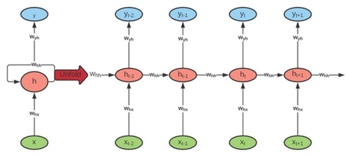
Recurrent Neural Network is an ANN class in which contacts neurons form a driven graph, or in simpler terms have a self-loop in the hidden layers. This allows RNNs to know the current state from the previous state of the hidden neurons. RNNs take the data they have recently learned in a period together with the current input instance. To learn sequential knowledge, they utilize the internal state or memory. This helps them to practice several tasks such as recognition of speech, recognition of handwriting, etc. Data can be moving in any direction and RNNs may use their internal memory to handle arbitrary input series. This might make RNN useful for solving more advanced and challenging tasks as well as for having higher computational complexity than feeding up neural networks. Thus, as shown in Figure 1 (Ozbayoglu, Gudelek, and Sezer 2020), we can unroll the network. This unrolled network illustrates how we can supply the RNN with a stream of data.

Figure 1. Recurrent neural network cell structure (Ozbayoglu, Gudelek, and Sezer 2020).

Long Short-Term Memory

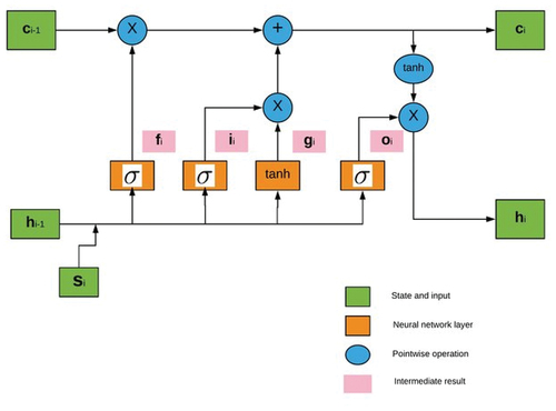
LSTM networks are an extension for recurrent neural networks that extend their memory essentially. it’s one of the most successful RNN’s architectures. Such networks are specifically designed to avoid the issue of long-term dependence but their normal behavior is to retain knowledge for a long-time period back. This is because LSTM’s store their information in memory similar to a computer’s memory since this network can read, write and remove information from its memory Hiransha et al. (2018). The LSTM model comprises a specific set of memory cells that replace the RNN’s hidden layer of neurons and its key is memory cell status. This model extracts information via the gate structure to retain and update the memory cell state. LSTM structure includes three gates: input, forget and output gate. Also, each memory cell has three layers of sigmoid and one layer of tanh. These gates decide whether to let new input into (input gate) or not, remove the information (i.e input) because it is not necessary (forget gate) or allow it to affect the output at the current time stage (output gate). In other words, the gates are used to manage and control the interaction of memory cells among themselves and neighbors. An illustration of the structure of LSTM memory cells with its three gates is shown in Figure 2.

Figure 2. Long short-term memory cells (Ozbayoglu, Gudelek, and Sezer 2020).

Convolutional Neural Network

The convolutional neural network is a kind of feed-forward ANN in which the pattern of connectivity among its neurons is influenced by the visual cortex of animals, the individual neurons are organized in such a way as to reply to overlapping areas tilting the visual field. Nonetheless, CNN architectures primarily focus on the provided input series and during the process of learning do not use any previous history or knowledge (Chen and He 2018). CNN is regarded to be the first truly successful and effective, multi-tiered hierarchical network-based DL method. The close linkage and temporal data between CNN layers make it particularly adequate for image processing and knowledge. So it can obtain rich correlation properties from the pictures automatically and instantly. CNN comprises a convolution layer, the layer of pooling, an active layer, interconnected layer as well as a layer of input-output. It holds structural features such as weight sharing, local connection, temporal or spatial sub-sampling, thereby making it preferable in image recognition. Figure 3 describes the structure of CNN with different layers.

Figure 3. Convolutional neural network structure (Albelwi and Ausif 2017).

The same as classical neural network architecture that includes input layers, hidden layers, and output layers, CNN also provides these features, and the input of the convolution layer is the output of the previous convolution or pooling layer. They obviously still have a few unique characteristics like pooling layers, fully connected layers, etc. In CNN, the number of hidden layers is more than that in a typical neural network, which to some degree demonstrates the neural network’s capability. Moreover, the more hidden layers are, the higher the feature it can retrieve and identify from the data.

Table 1 presents a listing of several deep learning researches on stock predictions.

Table 1. A comparative study of state-of-the-art of deep learning model for stock market prediction.

	Scope			Prediction Method					DS	Results
References	Market	Feature/s	Prediction/s	NN	RNN	LSTM	CNN	DRL	MASS	PM	Values
(AbdelKawy, Abdelmoez, and Shoukry 2021)	USA SM	OHLCV	stock			✓		✓	✓	APR	0.73
										AMDD	0.217
(Lee et al. 2020)	USA SM	close	stock				✓	✓	✓	Return	6.123
			price							Sharpe ratio	2.247
(Zhang, Zohren, and Roberts 2020)	SSE	CSI 300	stock					✓		SD	1.9586
		stock	return							Accuracy	0.038
(Kim and Won 2018)	korea	KOSPI 200	stock	✓		✓				MAE	0.46%
	stock	index	price							MSE	7.5%
	exchange									HMAE	29%
										HMSE	45.7%
(Hiransha et al. 2018)	NYSE	Close	stock		✓	✓	✓			MAPE	4.05
	NSE	Price	Price
(Chen and He 2018)	Chinese SM	OHLCV	stock				✓			Accuracy	75,2%
			Price							F1-score	73%
(Gurjar et al. 2018)	NSE	NIFTY 50	stock	✓						SD	-
		index	trend							MA	-
(Jain, Gupta, and Moghe 2018)	NSE	NIFTY 50	Market	✓						CE	6.13%
		index	direction
(Hu et al. 2018)	Chinese SM	Price	Stock	✓	✓					Accuracy	0.478
		Volume	Trend							ARR	0.611
(Fabbri and Moro 2018)	USA SM	DJIA	Stock		✓	✓				Accuracy	83%
		index	time series
(Minh et al. 2018)	USA SM	S&P 500	stock			✓				Accuracy	66.32%
		Index	trends							Precision	72.1%
										Recall	77.32%
(Liu, Zhang, and Ma 2017)	Chinese SM	Chinese	stock			✓	✓			ARR	0.309
		stocks	return
(Chong, Han, and Park 2017)	South Korea SM	KOSPI	stock	✓						RMSE	0.8214
		index	return							NMSE	0.9621
										MAE	0.5838
(Vargas, De Lima, and Evsukoff 2017)	USA SM	S&P 500	Market		✓		✓			Accuracy	64,21%
		Index	direction
(Roondiwala, Patel, and Varma 2017)	NSE	NIFTY 50	Stock		✓	✓				MSE	-
		Index	price
(Heaton, Polson, and Witte 2017)	NASDAQ	IBB	Market	✓						RMSE	2.36
		index	direction
(Selvin et al. 2017)	NSE	NIFTY IT	Stock		✓	✓	✓			RMSE	2.36
		index	price
(Huynh, Dang, and Duong 2017)	USA SM	S&P 500	Stock			✓				Accuracy	59.98%
		index	Price
(Bao, Yue, and Rao 2017)	Stock	S&P 500	stock		✓	✓
	markets	DJIA, HSI	price							MAPE	0.011
		Nifty 50								R	0.949
		CSI 300								Theil U	0.007
		Nikkeiindices
(Singh and Srivastava 2017)	NASDAQ	Close	stock		✓					Accuracy	43.4%
		price	Price							RMSE	0.007
										MAPE	0.08

Proposed Model

The proposed model built three different deep learning algorithms to predict the stock returns of the NIFTY 50 index using RNN, LSTM, and CNN. For sequential data tasks, these approaches are quite popular and display superior results to those of traditional deep learning techniques (Selvin et al. 2017). Our goal is to forecast the stock price of the NIFTY 50 index through time series prediction models based only on historical data. To design the suggested neural network models we need to follow some basic steps, namely, Data Collection and Preprocessing, feature extraction, model building and training. Finally, output generation and analysis based on different evaluation metrics.

Our methodology consists of several stages which are as follows:

1. Step 1 - Data collection (raw data): This study attempts to predict stock returns of the NIFTY 50 index concerning the stock’s previous value. It requires historical data on the stock market to create the prediction model. Therefore, it is essential to have a reliable source with data relevant and appropriate for the prediction. We used the Quandl website as the primary data source that represents a platform for financial and alternate data supplied to researchers and analysts currently in modern formats (such as Python, R, and Excel). This website contains all the historical data details that will be used for the prediction of future prices. It also provides the overall performance of NSE and the performance of companies of different categories. So, in this step we gathered 5 years of NIFTY 50 daily prices from the National stock exchange for the period of 01/01/2014 to 31/12/2018. The historical numeric data of stock price is collected from Quandl website. The dataset contains the daily price of each stock, daily open price, daily highest price, daily lowest price, and daily volume of trading also the daily change of trends. There are seven variables in the basic transaction dataset. This historical data is used for the prediction of future stock prices.

2. Step 2 - Data preprocessing: It is a very significant step toward getting some information from NIFTY 50 dataset to help us make the prediction. This step involves: a) Data discretization: We use data discretization to replace the raw values of the numeric attribute by interval levels. b) Data transformation: Data normalization is conducted before the start of the training process because non-linear activation functions tend to squash the node output either in (0, 1). To normalize or scale our data, we used $StandardScaler$ class from $sklearn.preprocessing$ library to scale our data between −1 and 1. This scaler allows us to standardize the feature by subtracting the mean and then scaling to unit variance. Also, we used the $featur{e}_{r}angeparameter$ to specify the range of the scaled data. The mathematical formula of $StandardScaler$ is as follows:

   $X_{scaled}=\frac{X-U}{S}$

With $U$ = mean of X feature $S$ = Standard deviation of X feature

c) Data cleaning: This step involves fill in missing values and delete duplicated data. d) Data splitting: After the dataset is transformed into a clean dataset, it is divided into training and testing sets to evaluate our models. The NIFTY 50 dataset is split into $80\mathrm{\%}$ for training and $20\mathrm{\%}$ for testing. Moreover, the training set is divided into training and validation sets using K-Fold cross-validation.

1. Step 3 - Feature selection: In this step, just the attributes that need to be fed to the neural network models are selected. In this research, we choose Date, Open, High, Low, Close and Volume. Each time we take a different combination of features for both the training and testing sets of each model. Since our work aims to analyze stock index using historical stock data, which consists of different attributes. Each one of them gives useful data or information that will help us in forecasting the stock index. So, instead of picking one feature such as close price. We wanted to try many sets of features, then we attempted to find out the best-extracted set of features that has the lowest error percentage using different DL techniques. This step will help us in predicting the stock index prices and choosing the best model with high accuracy.

2. Step 4 - Train the neural network models: The sequential deep neural network models are developed by providing the data set for the training. Modeling is initiated using biases and random weights and those models are trained on daily stock price data. Our RNN model is composed of 2 Simple RNN layers each with a dropout layer, followed by a dense layer and an output dense layer for making predictions. The LSTM model contains two LSTM layers each layer followed by a dropout layer and two dense layers. CNN model includes different type of layers that makes it different from RNN and LSTM. This model contains three convolution layers with a max-pooling layer, flatten layer that reduces the dimension, and reshapes input and two fully connected dense layers. Besides, one of the choices we need to make in the process of building a neural network is what activation function to use in the network’s layers. Therefore, we will examine three activation functions, namely (Sigmoid, ReLU, and Softmax) used in deep learning models. The choice of the activation function is most important for the output layer of each model as it will define the format that predictions will take. Their main purpose is to convert an input signal of a node in our neural networks to an output signal.

3. Step 5 - Output generation: Our neural networks generate their predictions in the form of a set of real values. Each output value is generated by one of the neurons in the output layer. The final part of our neural network is the output layer that produces the predicated value. The output value generated by the neural networks outputs layer is compared with the target value in this layer. Our neural network models need to use the back propagation algorithm to carry out iterative backward passes that aim to find the optimum perceptron weight values and generate the most accurate prediction. When the training is completed the neural network models are used to obtain the predictions on the test set. Then, those models are evaluated based on the outcomes from prediction. So to analyze the efficiency of the models we used different evaluation metrics.

Neural Networks Evaluation Metrics

Evaluation metrics are attached to the tasks of machine learning and since we are trying to predict future stock prices using deep learning approaches we need to use multiple evaluation metrics to examine and determine our model’s performance and behavior. We established a set of the most commonly used metrics which are (1) Accuracy, (2) the root mean square error (RMSE), (3) mean absolute error (MAE), (4) the mean square error (MSE) and (5) coefficient of determination (R²) for comparing and optimizing our prediction models. These criteria are preferred to be smaller since they indicate the prediction error of the models.

• Root Mean Square Error: It is the most commonly used evaluation metric for regression tasks. It supports the premise that error is unbiased. This is known as the square root between both the actual score and the expected score of the average squared distance and N represents the total number of data point. It is calculated as follows:

$RMSE=\sqrt{\frac{{\sum }_{t=1}^N(Y_t-{\hat{y}}_t)}{N}}$

The formula represents the distance between the real scores vector and the predicted scores vector, averaged by $\sqrt{N}$. $Y_t$ indicates the $t^{t}h$ data point’s true score, and ${\hat{y}}_t$ signifies the predicted value. N represents the total Number of data points. So, we choose RMSE because the power of ’ square root ’ allows this metric to reveal large variations in numbers. this metric helps us to deliver more robust results that prevent the positive and negative error values from being canceled.

• Mean Absolute Error: It is the average difference between both the true values and the values predicted. It provides us the measure of how far the forecasts from the actual output have come. In other words, this gives us an idea of how the forecasts were incorrect. This error metric is defined as follows:

$MAE=\frac{1}{N}\sum _{t=1}^N|Y_t-{\hat{y}}_t|$

• Mean Square Error: It is an estimator that calculates the average of squares of the errors. The term error in this metric describes the difference between the estimated value and the actual value. MSE is much like the MAE since the only distinction is that MSE uses the square average of the difference between the true values and the expected values. The equation below describes the mathematical formula used to measure the MSE.

$MSE=\frac{1}{N}\sum _{t=1}^N(Y_t-{\hat{y}}_t{)}^2$

In the equation above, $y_t$ is the vector of the true values and ${\hat{y}}_j$ is the vector of the values predicted. MSE is usually used when we have continuous-value vectors. The advantage of MSE is that the gradient is calculated more easily. We used this measure to compare the results of our models.

• Coefficient of determination (R²): The R-Squared metric shows the fit consistency of a series of predictions to the real values. It can show us how efficient our model of regression compared to a very simple model that only predicts the average target value from the train set as forecasts. The R² equation is as follows:

$R^2=1-\frac{{\sum }_{t=1}^N{(Y_t-{\hat{y}}_t)}^2}{{\sum }_{t=1}^N{({\bar{Y}}_t-{\hat{y}}_t)}^2}$

with ${\bar{Y}}_t$ is the empirical mean of Y feature.

We choose five different metrics to evaluate our models as well as to decide which model is the best that meets our target performance. Overall, these metrics try to measure not just the predictive power of our models but also their trade-ability, which is critically important for us because we intend to use our models in the real world.

Experimental Results and Discussions

This section represents the prediction results and observations obtained in the study. For this experiment, we used Keras library which is a high-level neural network API written in python and Tensorflow as a learning framework. Tensorflow is an open-source framework that offers various machine learning algorithms for numerical computation using data flow graphs. First, we perform our prediction using many combination of variables in order to insure feature selection. The latter affects machine learning performance as seen in the first subsection. Second, after fitting our model and choosing the relevant feature, we observe the stylized facts observed in our predicted index series.

Selecting Features and Machine Learning Results

Our experiment results for neural network models with the three activation functions are shown in table 2.

Table 2. Loss of neural network models.

Loss
Activation Function	RNN	LSTM	CNN
ReLu	0.6150	0.4705	0.6291
Sigmoid	0.6170	0.5203	0.6114
Softmax	0.6510	0.4828	0.7258

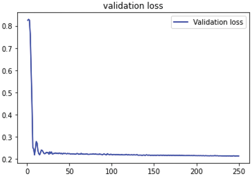
Table 2 shows that the use of Relu activation function for LSTM model could achieve the lowest loss of 0.4705 among Sigmoid and Softmax activation functions. However, the loss that we get from Sigmoid function is lower than the loss from other activation functions for CNN model by 0.6114. At last, ReLU is the best activation function with 0.4705 for the LSTM model. Figure 4 describes the evolution of the validation loss using LSTM with Relu function. This experiment was designed to detect which activation function is more suitable for each model. For the rest of experiments, we will use Relu for RNN and LSTM and Sigmoid for CNN models.

Figure 4. Validation Loss of LSTM model using Relu activation function.

The training and testing are performed by batches using input random data samples. The number of data is affected by multiple batches similarly. By identifying the input and its related output the batches train the network. This process is carried out for all batches, and a completely performed batch is an epoch. we used different evaluation metrics to examine our models. This is because our models can perform well just by using one metric but may do inadequately using another metric. We evaluated MSE, RMSE, MAE, and R² predictive results for each model. The smaller the MSE, RMSE, and MAE, the closer the forecasted value to the true value. The closer the coefficient R² to 1, the better the fit of the model. In our experiment, we compare the training set of the LSTM model we designed with different types of evaluation metrics. We have used several set of features with a different number of epochs to measure the model error.

According to Table 3, the best evaluation metric of LSTM training set is RMSE with 0.004 of error percentage. Also, we can notice that the best features set is (High/Low/Open/Close) with 500 epochs. For R², the best result is 0.673 of error percentage and the best features set is (High/Low/Open/Close) with 250 epochs.

Table 3. Error value for LSTM training set.

Features	Epoc.	RMSE	MSE	MAE	R^2
O – C	250	0.012	0.025	0.035	0.31
O – C	500	0.035	0.048	0.027	0.36
H - L – C	250	0.015	0.016	0.061	0.51
H - L- C	500	0.011	0.026	0.054	0.21
H - L- O- C	250	0.053	0.049	0.073	0.67
H - L - O – C	500	0.004	0.008	0.006	0.54
H - L - O - C- V	500	0.005	0.009	0.008	0.37

As shown in Table 4, the best metric to evaluate LSTM testing set is RMSE with 0.002 of error percentage. Thus, the best features set are (High/Low/Open/Close) with 500 epochs. In addition, the best result of error percentage for R2 is 0.537 with the features set of (High/Low/Open/Close) and 250 epochs. Figure 5 plots the Nifty 50 prices. The black line represents the actual stock prices, while the red line represents the predicted stock prices. According to the chart above, we can notice that there are high volatility periods, even though we have low volatility periods. Thus, every period of high volatility started with a decline in returns. This figure shows that the LSTM network was successful in capturing the pattern between the period of 200 and 400 days but between the period of 600 and 800 days LSTM failed to identify the seasonal pattern that can be considered as change in behavior of system. Similarly for the RNN model, we compare the results we obtained from both training and testing sets with the same types of evaluation metrics. As well as, we used the same features set and the number of epochs to calculate the model error.

Figure 5. Real value vs Predicted value for NIFTY 50 using RNN .

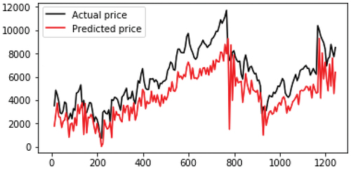
Table 4. Error value for LSTM testing set.

Features	Epoc.	RMSE	MSE	MAE	R^2
O – C	250	0.044	0.062	0.081	0.528
O – C	500	0.055	0.051	0.067	0.341
H - L – C	250	0.037	0.023	0.032	0.516
H - L – C	500	0.063	0.053	0.034	0.201
H - L - O – C	250	0.082	0.057	0.063	0.537
H - L - O – C	500	0.002	0.009	0.006	0.482
H - L - O - C – V	500	0.004	0.005	0.002	0.247

Table 5 shows the results obtained from the RNN training set with the different evaluation metrics. The best result is 0.004 of error percentage from MSE metric with 500 epochs by taking four features set (High/Low/Open/Close). For R², the best result is 0.578 of error percentage with (High/Low/Close) features set and 250 epochs.

Table 5. Error value for RNN training set.

Features	Epoc.	RMSE	MSE	MAE	R^2
O – C	250	0.014	0.085	0.072	0.401
O – Close	500	0.035	0.073	0.015	0.351
H - L – C	250	0.063	0.092	0.048	0.578
H - L – C	500	0.028	0.052	0.038	0.427
H - L - O – C	250	0.069	0.064	0.083	0.563
H - L - O – C	500	0.007	0.004	0.009	0.358
H - L - O - C – V	500	0.006	0.005	0.007	0.497

As observed from Table 6, the best evaluation metrics for the RNN testing set are MSE with 0.00347 of error percentage and R2 with 0.810 of error percentage. Besides, the best features set is (High/Low/Close) with 250 epochs.

Table 6. Error value for RNN testing set.

Features	Epoc.	RMSE	MSE	MAE	R^2
O – C	250	0.029	0.058	0.037	0.485
O – C	500	0.045	0.057	0.057	0.274
H - L – C	250	0.047	0.059	0.045	0.810
H - L – C	500	0.079	0.047	0.048	0.389
H - L - O – C	250	0.047	0.037	0.036	0.584
H - L - O – C	500	0.007	0.003	0.007	0.804
H - L - O - C – V	500	0.007	0.006	0.004	0.638

Figure 5 shows the real and predicted values nifty 50 stocks using RNN, we can notice a no linear auto-correlation. In other words, there’s an auto-correlation between real and predicted values. In addition, n this figure, RNN was almost successful in identifying the pattern in the period of 200 days but between the time period 400 and 1000 days it failed to capture the pattern. Looking at the RNN and LSTM graphs, we clearly observe that predicted values are behind the actual data, which implies that our neural networks can follow the trend, but cannot predict the exact future values of stock prices. Moreover, the above graphs are showing a poor result in terms of curve fitting. This has a clear justification. For time-series of stock price data. LSTM is better suited to learn temporal patterns in deep neural networks. Since it uses memory cells (states) and (input and forget) gates. So, LSTM represents a better option for future predictions then RNN.

As shown from the given results in Table 7, the best metric to evaluate our CNN training set model is MAE with 0.014 of error percentage. As for R2 the best error percentage is 0.819. Also, we have observed that the best set of features is (High/Low/Open/Close) with 500 number of epochs for MAE metric and the best features set for R2 is (High/Low/Open/Close) with 250 number of epochs.

Table 7. Error value for CNN training set.

Features	Epoc.	RMSE	MSE	MAE	R^2
O – C	250	0.013	0.017	0.017	0.359
O – C	500	0.018	0.026	0.047	0.642
H - L – C	250	0.018	0.017	0.025	0.361
H - L – C	500	0.032	0.024	0.034	0.675
H - L - O – C	250	0.039	0.024	0.074	0.819
H - L - O – C	500	0.016	0.015	0.014	0.520
H - L - O - C – V	500	0.017	0.016	0.015	0.371

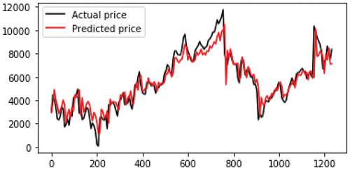
In Figure 6, we have displayed the results related to the training of LSTM architecture. This figure shows that the LSTM was successful in capturing the pattern in all the period but it almost captured the pattern between the period of 600 and 800 days. Also, we can observe that LSTM performed better compared to other three networks. So, it is clear that, from this perspective, LSTMs are the best choice for modeling financial time series. Such a result suggests us to use LSTM as basic predictor. We used multivariate data that includes stock prices of more than one company for various instances of time. Analysis of time series data helps in identifying patterns, trends and periods or cycles existing in the data. So through the time series, we can track the movement of the chosen data points over a specified period using the architectures described in the previous sections.

Figure 6. Real value vs predicted value for NIFTY 50 using LSTM .

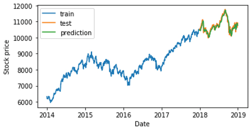
In Figures 7, 8 and 9, we report a graphical visualization of obtained predictions of close prices over early 2014. From these figures, we can observe that the LSTM prediction model was almost successful in forecasting the future direction of NIFTY 50 close prices.

Figure 7. Prediction of close price using RNN.

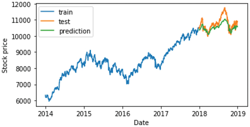
Figure 8. Prediction of close price using CNN.

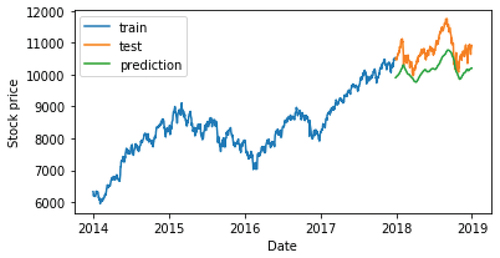
Figure 9. Prediction of close price using LSTM.

Conclusion and Future Works

In this research, different neural network approaches, namely RNN, LSTM, and CNN, have been applied to the forecasting of stock market price movements. This study discusses the use of neural networks to predict future stock price patterns focused on historical prices. We focused on the importance of choosing the correct input features, along with their preprocessing, for the specific learning models and predicting trend on the basis of data from the past 5 years. For analyzing the efficiency of our models we used four different evaluation metrics. For each model, we measure the error percentage that exists in the training and testing dataset. Then, we compare the obtained results using various sets of features with a specific number of epochs. After we conducted several experiments with different features and epochs, we have found that LSTM is the best model. As we have established through our work that deep learning can stably predict the stock price movement, we think there is more scope to work on making the investment more dynamic and intelligently responsive to the market. We can combine many models for better prediction and efficiency. Besides, the models in this experiment can be updated with other stock indices and they can be optimized using hyper-parameter optimization. In the future, it could be possible to combine multi-agent system and our deep learning methods to enhance predicting the exact price value.

Disclosure statement

No potential conflict of interest was reported by the author(s).

References

- AbdelKawy, R., W. M. Abdelmoez, and A. Shoukry. 2021. A synchronous deep reinforcement learning model for automated multi-stock trading. Progress in Artificial Intelligence 10 (1):83–3123. doi:10.1007/s13748-020-00225-z.
- Abinaya, P., V. S. Kumar, P. Balasubramanian, and V. K. Menon (2016). Measuring stock price and trading volume causality among nifty50 stocks: The toda yamamoto method. In 2016 International Conference on Advances in Computing, Communications and Informatics (ICACCI), pp. 1886–90. IEEE.
- Albelwi, S., and M. Ausif. 2017. A framework for designing the architectures of deep convolutional neural networks. Entropy 19 (6):242. doi:10.3390/e19060242.
- Alkhoshi, E., and B. Saeid (2018). Stable stock market prediction using narx algorithm. In Proceedings of the 2018 International Conference on Computing and Big Data, pp. 62–66.
- As, S. 2013. A study on fundamental and technical analysis. International Journal of Marketing, Financial Services & Management Research 2 (5):44–59.
- Ashfaq, R. A., W. Xi-Zhao, H. J. Zhexue, A. Haider, and H. Yu-Lin. 2017. Fuzziness based semi-supervised learning approach for intrusion detection system. Information Sciences 378:484–97. doi:10.1016/j.ins.2016.04.019.
- Aziz, T., and A. V. Ahmad. 2018. Are extreme negative returns priced in the indian stock market? Borsa Istanbul Review 18 (1):76–90. doi:10.1016/j.bir.2017.09.002.
- Bao, W., J. Yue, and Y. Rao. 2017. A deep learning framework for financial time series using stacked autoencoders and long-short term memory. PloS One 12 (7):e0180944. doi:10.1371/journal.pone.0180944.
- Checkley, M., D. A. S. Higón, and H. Alles. 2017. The hasty wisdom of the mob: How market sentiment predicts stock market behavior. Expert Systems with Applications 77:256–63. doi:10.1016/j.eswa.2017.01.029.
- Chen, S., and H. He (2018). Stock prediction using convolutional neural network. In IOP Conference series: materials science and engineering, Volume 435, pp. 012026. IOP Publishing.
- Chong, E., C. Han, and F. C. Park. 2017. Deep learning networks for stock market analysis and prediction: Methodology, data representations, and case studies. Expert Systems with Applications 83:187–205. doi:10.1016/j.eswa.2017.04.030.
- Chou, J., and N. Thi-Kha. 2018. Forward forecast of stock price using sliding-window metaheuristic-optimized machine-learning regression. IEEE Transactions on Industrial Informatics 14 (7):3132–42. doi:10.1109/TII.2018.2794389.
- Dahir, A. M., M. Fauziah, A. R. N. Hisyam, and B. A. An. 2018. Revisiting the dynamic relationship between exchange rates and stock prices in brics countries: A wavelet analysis. Borsa Istanbul Review 18 (2):101–13. doi:10.1016/j.bir.2017.10.001.
- Drakopoulou, V. 2016. A review of fundamental and technical stock analysis techniques. Journal of Stock & Forex Trading 5. doi: 10.4172/2168-9458.1000163.
- Fabbri, M., and G. Moro. 2018. Dow jones trading with deep learning: The unreasonable effectiveness of recurrent neural networks. Data 142–53.
- Fama, E. F. 1970. Efficient capital markets: A review of theory and empirical work. The Journal of Finance 25 (2):383–417. doi:10.2307/2325486.
- Fama, E. F. 1995. Random walks in stock market prices. Financial Analysts Journal 51 (1):75–80. doi:10.2469/faj.v51.n1.1861.
- Gurjar, M., P. Naik, G. Mujumdar, and T. Vaidya. 2018. Stock market prediction using ann. International Research Journal of Engineering and Technology 5 (3):2758–61.
- Heaton, J. B., N. G. Polson, and J. H. Witte. 2017. Deep learning for finance: Deep portfolios. Applied Stochastic Models in Business and Industry 33 (1):3–12. doi:10.1002/asmb.2209.
- Hiransha, M., E. A. Gopalakrishnan, V. K. Menon, and K. Soman. 2018. Nse stock market prediction using deep-learning models. Procedia Computer Science 132:1351–62. doi:10.1016/j.procs.2018.05.050.
- Hu, Z., W. Liu, J. Bian, X. Liu, and T.-Y. Liu (2018). Listening to chaotic whispers: A deep learning framework for news-oriented stock trend prediction. In Proceedings of the eleventh ACM international conference on web search and data mining, pp. 261–69.
- Huynh, H. D., L. M. Dang, and D. Duong (2017). A new model for stock price movements prediction using deep neural network. In Proceedings of the Eighth International Symposium on Information and Communication Technology, pp. 57–62.
- Jain, S., R. Gupta, and A. A. Moghe (2018). Stock price prediction on daily stock data using deep neural networks. In 2018 International conference on advanced computation and telecommunication (ICACAT), pp. 1–13. IEEE.
- Khedr, A. E., N. Yaseen, and N. Yaseen. 2017. Predicting stock market behavior using data mining technique and news sentiment analysis. International Journal of Intelligent Systems and Applications 9 (7):22. doi:10.5815/ijisa.2017.07.03.
- Kim, H. Y., and C. H. Won. 2018. Forecasting the volatility of stock price index: A hybrid model integrating lstm with multiple garch-type models. Expert Systems with Applications 103:25–37. doi:10.1016/j.eswa.2018.03.002.
- Kumar, D. A., and S. Murugan (2013). Performance analysis of indian stock market index using neural network time series model. In 2013 International Conference on Pattern Recognition, Informatics and Mobile Engineering, pp. 72–78. IEEE.
- Lee, J., R. Kim, S.-W. Yi, and J. Kang. 2020. Maps: Multi-agent reinforcement learning-based portfolio management system. arXiv preprint arXiv:200705402.
- Liu, S., C. Zhang, and J. Ma (2017). Cnn-Lstm neural network model for quantitative strategy analysis in stock markets. In international conference on neural information processing, pp. 198–206. Springer.
- Lv, D., Y. Shuhan, L. Meizi, and Y. Xiang. 2019. An empirical study of machine learning algorithms for stock daily trading strategy. Mathematical Problems in Engineering 2019. doi:10.1155/2019/7816154.
- Malkiel, B. G. 2005. Reflections on the efficient market hypothesis: 30 years later. Financial Review 40 (1):1–9. doi:10.1111/j.0732-8516.2005.00090.x.
- Milosevic, N. 2016. Equity forecast: Predicting long term stock price movement using machine learning. arXiv preprint arXiv:160300751.
- Minh, D. L., A. Sadeghi-Niaraki, H. D. Huy, K. Min, and H. Moon. 2018. Deep learning approach for short-term stock trends prediction based on two-stream gated recurrent unit network. IEEE Access 6:55392–404. doi:10.1109/ACCESS.2018.2868970.
- Nti, I. K., A. A. Felix, and W. B. Asubam. 2020. A systematic review of fundamental and technical analysis of stock market predictions. Artificial Intelligence Review 53 (4):3007–57. doi:10.1007/s10462-019-09754-z.
- Ozbayoglu, A. M., M. U. Gudelek, and O. B. Sezer. 2020. Deep learning for financial applications : A survey. Applied Soft Computing 93:106384. doi:10.1016/j.asoc.2020.106384.
- Putriningtiyas, D. A., and A. M. Mochammad. 2017. Analysis effectiveness of moving average convergence divergence (macd) in determining buying and selling decision of stock. Jurnal Administrasi Bisnis (JAB) 53 (1).
- Roondiwala, M., H. Patel, and S. Varma. 2017. Predicting stock prices using lstm. International Journal of Science and Research (IJSR) 6 (4):1754–56.
- Selvin, S., R. Vinayakumar, E. Gopalakrishnan, V. K. Menon, and K. Soman (2017). Stock price prediction using lstm, rnn and cnn-sliding window model. In 2017 International Conference on Advances in Computing, Communications and Informatics (ICACCI), pp. 1643–47. IEEE.
- Singh, R., and S. Srivastava. 2017. Stock prediction using deep learning. Multimedia Tools and Applications 76 (18):18569–84. doi:10.1007/s11042-016-4159-7.
- Soui, M., S. Smiti, M. W. Mkaouer, and R. Ejbali. 2020. Bankruptcy prediction using stacked auto-encoders. Applied Artificial Intelligence 34 (1):80–100. doi:10.1080/08839514.2019.1691849.
- Tsai, M. F., and C. J. Wang. 2017. On the risk prediction and analysis of soft information in finance reports. European Journal of Operational Research 257 (1):243–50. doi:10.1016/j.ejor.2016.06.069.
- Vargas, M. R., B. S. De Lima, and A. G. Evsukoff (2017). Deep learning for stock market prediction from financial news articles. In 2017 IEEE international conference on computational intelligence and virtual environments for measurement systems and applications (CIVEMSA), pp. 60–65. IEEE.
- Xiang, H., X. Xu, H. Zheng, S. Li, T. Wu, W. Dou, and S. Yu (2016). An adaptive cloudlet placement method for mobile applications over gps big data. In 2016 IEEE Global Communications Conference (GLOBECOM), pp. 1–6. IEEE.
- Zhang, X., G. Naijie, C. Jie, and Y. Hong. 2021. Predicting stock price movement using a dbn-rnn. Applied Artificial Intelligence 35 (12):876–92. doi:10.1080/08839514.2021.1942520.
- Zhang, J., C. Shicheng, X. Yan, L. Qianmu, and L. Tao. 2018. A novel data-driven stock price trend prediction system. Expert Systems with Applications 97:60–69. doi:10.1016/j.eswa.2017.12.026.
- Zhang, Z., S. Zohren, and S. Roberts. 2020. Deep reinforcement learning for trading. The Journal of Financial Data Science 2 (2):25–40. doi:10.3905/jfds.2020.1.030.