Visual inspection of surface defects of extreme size based on an advanced FCOS

ABSTRACT

Surface defects of industrial products are generally detected through anchor-based object detection methods during manufacturing. However, these methods are prone to missed and false detection for ultra-elongated and ultra-fine defects. An advanced fully convolutional one-stage object detector (FCOS) is proposed. This method is based on an anchor-free FCOS network model. First, a novel type of center-ness is proposed to reduce the suppression of off-centered positions of defects of extreme size. In addition, to eliminate background interference, a self-adaptive center sampling method is proposed as a replacement for the conventional center sampling method. The regularization method and the loss function are also improved according to the defect characteristics. Experimental results show that this advanced-FCOS-based method outperforms anchor-based methodson the surface defect dataset. The proposed method effectively detects defects of extreme size without affecting the detection of normal defects. The performance of the proposed method meets the requirements of real industrial applications.

Introduction

Surface defects not only affect the appearance of a product but may also cause serious safety problems during the use process. In recent years, machine vision-based detection methods (Wang et al. 2018; Kwon et al. 2015) have received extensive attention due to their high detection accuracy and fast detection speed. This type of method involves first the collection of product surface images via an industrial camera and then the processing of the images with conventional image processing or deep learning methods to obtain the corresponding results.

Compared with conventional image processing methods, deep learning-based defect detection methods have a wider range of adaptability. A network can be trained on samples with different types of defects for use in the detection of multiple types of defects. Liu and Kang (2005) proposed a neural-network-based method for cold rolled strips, but this method cannot effectively locate defects. With the proposed object detection framework, deep learning methods can be used to accurately locate various defects. Ji, Du, and Peng et al. (2019) used the Faster region-based convolutional neural network (R-CNN) to detect defects in gears, which is faster and more accurate than previous methods. Zhang and Huang (2020) integrated Faster R-CNN and You Only Look Once (YOLO) v3 for the detection of aluminum surface defects.

The abovementioned methods are anchor-based. These methods can often effectively detect defects with a normal aspect ratio. However, these methods can only partially detect or even fail to detect defects of extreme size, such as elongated defects or microdefects. In this study, a defect with a label box aspect ratio greater than n (e.g., n > 5) or a label box area satisfying the ratio of the number of pixels in the label box to the number of pixels in the original image ≤ f (e.g., f = 1 × 10⁻⁴) is defined as a defect of extreme size. This type of defect often exists on large parts, such as engine blades or wind turbine blades. Normal defects with a large overall size are also considered to be extreme-size defects, for which anchor-based methods cannot enumerate all the label boxes. Therefore, an advanced-FCOS-based anchor-free detection method is proposed in this study to solve this problem.

The main contributions of this paper are as follows:

1. An anchor-free detection method is proposed to solve the problem that extreme-size targets are difficult for the existing network to detect without affecting the detection of normal-size defects.

2. To alleviate excessive suppression of slender defects by the original center-ness, the center-ness index term is modified to improve adaptability to slender defects.

3. Adaptive central sampling is proposed to reduce the loss of information for extreme-size defects caused by central sampling.

The rest of the paper is organized as follows: the recent research advances in this field are described in Section 2. An overview of the methodology of the advanced FCOS is presented in Section 3. Experimental results are presented and discussed in Section 4. Conclusions are presented in Section 5.

Related Work

Object detection in machine vision refers to finding the position of an object of interest in an image and classifying the object. This task is highly challenging because of the large variety and complexity of shapes of objects and the presence of background interference in industrial scenes.

Conventional object detection uses a sliding window in conjunction with a classifier method. Each time the sliding window slides to a region, the classifier determines the category of the region. Chen and Liu (2007) and Han and Liao (2009) used the Harr feature and the AdaBoost classifier to detect human faces. Bauer, Köhler, and Doll et al. (2010) proposed a pedestrian detection method based on a support vector machine (SVM). Wang, Jia, and Huang et al. (2008) and Gan and Cheng (2011) investigated object detection methods based on a histogram of oriented gradients (HOG) for pedestrian detection. These methods require feature representation to be manually designed based on experience.

Deep learning methods were first used in image classification. AlexNet (Krizhevsky, Sutskever, and Hinton 2017), VGG (Simonyan and Zisserman 2014), and ResNet (He, Zhang, and Ren et al. 2016) were shown to far outperform other conventional image classification methods on the ImageNet dataset. Subsequently, an R-CNN (Girshick, Donahue, and Darrell et al. 2014) was used to locate objects using a selective search algorithm with an SVM classifier, and a deep convolutional network was used for end-to-end object detection. Generally, deep-learning-based object detection methods are classified into two categories. One category includes two-stage methods, such as Fast R-CNN (Girshick 2015) and Faster R-CNN (Ren, He, and Girshick et al. 2015). The other category includes one-stage methods, such as YOLO (Redmon and Farhadi 2017; Redmon, Divvala, and Girshick et al. 2016) and single-shot detection (SSD) (Liu, Anguelov, and Erhan et al. 2016). Two-stage methods are based on R-CNN. These methods first generate the object candidate box, then classify the candidate box, and perform regression on the coordinate offset of the candidate box. These methods are more accurate but are less efficient. In contrast, the one-stage methods directly regress the object position and the probability of its category. Although the one-stage methods generally have lower accuracy than the two-stage methods, their detection speed is faster. A feature pyramid network (FPN) (Lin, Dollar, and Girshick et al. 2017) was proposed to simultaneously make predictions on multiple scales, thus improving the performance of the network for detecting small objects. The methods mentioned above are all anchor-based.

An anchor is a prediction box with a fixed shape and size obtained by clustering ground truth labeled boxes, which can avoid blind searching during model training and help the model converge quickly. For example, Faster R-CNN needs manual specification of the anchor parameter ratio and scale and obtains a series of anchors through different combinations of these two parameters, while YOLOv3 (Redmon and Farhadi 2018) obtains the widths and heights (dimension clustering) of representative shapes to form the anchors by clustering the ground truth of all samples in the training set via the k-means algorithm. These anchors mark the detection object in a rectangular box, and the horizontal and vertical axes of the box are parallel to the horizontal and vertical directions of the image. The shape and size of the rectangular box need to be determined by prior knowledge from the ground truth. Therefore, when the size and aspect ratio of the object change drastically, the performance of the model declines sharply. For example, when there are defects such as elongated scratches and microspots, the anchor-based method is prone to missed detection and misdetection. In addition, the exhaustive number of rectangular boxes must be increased to improve the detection accuracy for such defects, which increases the detection time. The experiments in this paper confirm that Faster R-CNN and YOLO have limitations in detecting defects of extreme size.

Therefore, to achieve better detection results, anchor values should be setted properly or a customized anchor-based architecture should be built. DefectDet (Duje et al. 2022) modified the detection head to improve the detection of the objects with extreme aspect ratios which are common in UT images. Another way is to free the network from the constraint of anchors. The first anchor-free model DenseBox (Huang, Yang, and Deng et al. 2015) first introduced the concept of a fully convolutional network (FCN) (Shelhamer, Long, and Darrell 2017) into target detection. The model directly predicts the bounding box and confidence score of each pixel result through NMS. CenterNet (Zhou, Wang, and Krahenbühl 2019) and FCOS (Tian, Shen, and Chen et al. 2019) are the most representative anchor-free methods. CenterNet replaces the object with its center point and ultimately returns the position of the center point and the object size. An FCOS is similar to CenterNet, but it returns a series of points close to the center point of the object and the distance from this point to the object bounding box. In CenterNet, a target corresponds to the local peak point on the feature map output by the network. This network does not provide an effective solution to overlapping targets. Comparing the two types of methods, an FCOS is more likely to have the ability to detect objects of extreme size. Therefore, an FCOS is used in this study as a backbone for the detection of defects in industrial products. The original network structure is improved to improve the detection performance for extreme-size defects.

Advanced FCOS Network Structure and Algorithm Design

Original FCOS

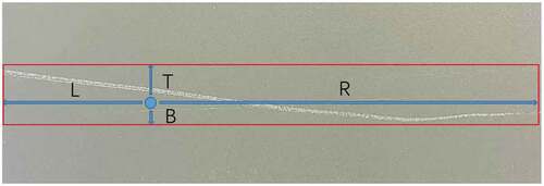
For the anchor-based methods, it is necessary to generate a large number of anchors and gradually fit an object through these anchors, while an FCOS predicts the sampling points by using the concept of FCN to obtain the corresponding category of each sampling point and the distances from each sampling point to the four sides of the corresponding object bounding box, as shown in Figure 1.

Figure 1. Schematic diagram of the FCOS prediction results.

Let $F_i\in R^{H\times W\times C}$ represent the feature map of the ith layer in the convolutional neural network (CNN) backbone and s represent the total stride from the input image to this layer. In the $F_i$ layer, a certain position (x, y) corresponds to an area centered at (s/2 + xs, s/2 + ys) on the input image.

For the FCOS, if the position (x, y) falls in a certain ground truth box, it is considered a positive sample belonging to this category; otherwise, it is regarded as a negative sample, that is, background. In the FCOS, C binary classifiers (C is the total number of categories) are trained rather than one multiclassifier. Moreover, to describe the prediction results, in addition to the classification label of the position, the FCOS regresses a four-dimensional vector (L, T, R, B), where L, T, R, and B represent the distances from the position to the four sides of the bounding box, as shown in Figure 1. The network structure of the FCOS in Figure 2 shows that regression and classification are output as two branches. As the distance obtained by the regression is always positive, the output of the model is mapped through the exponential function at the top of the regression branch. If a position exists in multiple ground truth boxes at the same time, its category attribution is ambiguous, that is, a position belongs to multiple categories at the same time; however, the final output of the classifier should be one category.

Figure 2. FCOS network structure diagram.

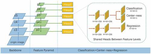
To eliminate the ambiguity of overlapping objects, the bounding box with minimal area is chosen as its regression target. Moreover structure of an FPN is introduced in the FCOS, with different levels of the FPN predicting objects of different sizes. The FPN has a total of five feature levels, namely, P3, P4, P5, P6, and P7. By limiting the regression results of each layer (i.e., L, R, T, and B in Figure 1), the model assigns a task of predicting objects of a different size to each layer, thereby avoiding the problem of overlap between objects of different sizes. Specifically, if max(L, T, R, B)>m_i or max(L, T, R, B) <m _i-1, this position is set as the background in this layer. Here, m_i represents the maximum regression distance of the ith feature layer, and m₂, m₃, m₄, m₅, m₆, and m₇ are generally set to 0, 64, 128, 256, 512, and ∞, respectively.

In addition to the output classification and regression common to the object detection models, the FCOS outputs the center-ness to suppress the bounding boxes that are close to the edge of the object. The center-ness represents the distance between a position and the center of the object. The center-ness of the object center is 1, and the greater the distance of the position from the center, the smaller its center-ness. During inference, the center-ness is combined with the category confidence to calculate a final score. At the nonmaximum suppression (NMS) stage, filtering is performed based on the final score so that these prediction boxes that are far from the center can be filtered out. The expression of center-ness c_x,y is as follows:

(1) $c_{x,y}=(\frac{min(l,r)}{max(l,r)}\times \frac{min(t,b)}{max(t,b)}{)}^{\frac{1}{2}}$(1)

In Equation (1)(1) $c_{x,y}=(\frac{min(l,r)}{max(l,r)}\times \frac{min(t,b)}{max(t,b)}{)}^{\frac{1}{2}}$(1) , the square root operation is to reduce the attenuation rate of the center-ness. Since the value range of center-ness is [0, 1], binary cross-entropy loss is used for training. In the testing phase, the ranking score of the NMS is taken as follows:

(2) $s_{x,y}=\sqrt{p_{x,y}\times c_{x,y}}$(2)

where $p_{x,y}$ represents the classification score.

The loss function of the FCOS is as follows:

(3) $L(\{p_{x,y}\},\{t_{x,y}\})=\frac{1}{N_{\mathrm{p}\mathrm{o}\mathrm{s}}}\sum _{x,y}{L}_{\mathrm{c}\mathrm{l}\mathrm{s}}(p_{x,y},c_{x,y}^{\ast })+\frac{\lambda }{N_{\mathrm{p}\mathrm{o}\mathrm{s}}}\sum _{x,y}{l}_{\{c_{x,y}^{\ast }>0\}}{L}_{\mathrm{r}\mathrm{e}\mathrm{g}}(t_{x,y},t_{x,y}^{\ast })$(3)

where L_cls is the classification loss, which is represented by the focal loss (Linet al. 2017), and L_reg is the regression loss. N_pos represents the number of positive samples, and positive samples are the sample points that fall within the label box. Λ is a hyperparameter with a default value of 1.

Improved Center-Ness

For elongated defects, such as the scratches shown in Figure 3(a), a very large aspect ratio causes the center-ness defined in (1) to be very sensitive to changes in the short side but less sensitive to changes in the long side. Thus, a large number of bounding boxes close to the ground truth are suppressed in the NMS stage, resulting in missed detection of elongated defects.

Figure 3. Schematic diagram and the center-ness heatmap of an elongated defect (a) Schematic diagram of elongated defects (b) Heatmap of the original center-ness (c) Heatmap of the improved center-ness.

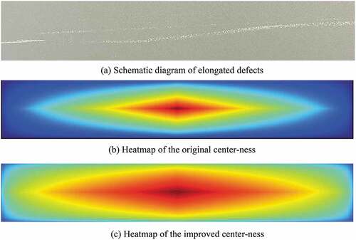
As shown in Figure 3(b), the predicted values in the narrow red range at the center are retained, while the predicted values in the surrounding large range are suppressed and filtered in the NMS stage. In fact, these positions can also describe the defect well and are not the so-called low-quality prediction boxes. Consequently, a novel definition of center-ness is proposed:

(4) $c_{x,y}=(\frac{min(l,r)}{max(l,r)}\times \frac{min(t,b)}{max(t,b)}{)}^{\alpha }$(4)

(5) $\alpha =\frac{min(h,w)}{2max(h,w)}$(5)

where h and w denote the height and the width of the bounding box, respectively. When the aspect ratio increases, α decreases, and in this manner, the suppression of the prediction boxes of elongated defects can be weakened. For nonelongated defects, the improved center-ness can also suppress the off-center bounding boxes as the original center-ness does. As shown in Figure 3(c), the improved center-ness has a better tolerance in the width direction, which weakens the excessive suppression of the predicted values in the width direction of elongated defects by the original center-ness.

In addition, the center-ness and classification modules in the conventional FCOS share parameters, as Figure 2 shows. In this study, the center-ness branch and regression branch are implemented together, as in (Tian et al. 2020), after the center-ness is improved. The advanced FCOS network structure is shown in Figure 4.

Figure 4. Advanced FCOS structure.

Self-Adaptive Center Sampling

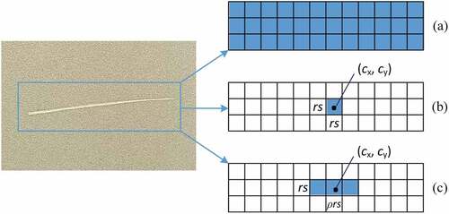
In the conventional FCOS, the sample points that fall into the ground truth labeled box are treated as positive samples, which causes many positive samples to deviate from the center of the object. These samples introduce a large quantity of background information and affect the detection results, as shown in Figure 5(a). Tian et al. (2020) used center sampling to improve this problem, as shown in Figure 5 (b). Specifically, only the points in the central region of the object are treated as positive samples. The central region is defined as (c_x – rs; c_y – rs; c_x + rs; c_y + rs). c_x and c_y represent the abscissa and ordinate coordinates of the center point, respectively, s represents the stride of the FPN layer, and r is a hyper-parameter with a default value of 1.5. However, this sampling method loses most of the information for elongated objects. Therefore, a self-adaptive center sampling method is proposed in this study to redefine the center region as (c_x – rs; c_y – ρrs; c_x + rs; c_y + ρrs) when ρ ≤ 1, or (c_x – ρrs; c_y – rs; c_x + ρrs; c_y + rs) when ρ > 1, where ρ represents the aspect ratio of the label box and the definitions of the remaining symbols remain unchanged, as shown in Figure 5 (c). It will work for objects elongated in all the directions according to ρ. After the improvement, as the aspect ratio of the label box changes, the central area changes accordingly so that the part that deviates in the length direction can also be used as a positive sample instead of the background.

Figure 5. Schematic of center sampling and self-adaptive center sampling. (a) Original FCOS sampling. (b) Center sampling. (c) Self-adaptive center sampling.

Using the GIoU Loss Function

The regression branch of conventional FCOS uses the intersection over union (IoU) loss as the loss function (Yu, Jiang, and Wang et al. 2016). However, there are two problems with using IoU loss as the loss function. First, when two bounding boxes do not intersect, the IoU is 0 regardless of the distance. However, the closer the bounding boxes are, the more accurate the prediction of the model should be, but the IoU loss cannot reflect this trend. Second, when two bounding boxes intersect, the prediction accuracy is not only related to the intersection area but also related to the intersection position, which is also not affected by the IoU loss. Therefore, this study uses the generalized intersection over union (GIoU) loss (Rezatofighi, Tsoi, and Gwak et al. 2019) instead of IoU loss.

Assuming that there are two bounding Boxes A and B, then

(6) $\mathrm{I}\mathrm{o}\mathrm{U}=(A\cap B)/(A\cup B)$(6)

The minimum closure region of A and B is defined as C; then, the GIoU formula is as follows:

(7) $\mathrm{G}\mathrm{I}\mathrm{o}\mathrm{U}=\mathrm{I}\mathrm{o}\mathrm{U}-\frac{(A\cup B)}{\mathrm{C}}$(7)

The GIoU loss is hence as follows:

(8) $L_{\mathrm{G}\mathrm{I}\mathrm{o}\mathrm{U}}=1-\mathrm{G}\mathrm{I}\mathrm{o}\mathrm{U}$(8)

Through the definition of GIoU, it can be seen that GIoU takes into account both the overlapping and nonoverlapping regions of the two intersecting bounding boxes as well as the situation of two bounding boxes that do not intersect, which makes up for the deficiency of using IoU as the loss function.

Group Normalization

The original FCOS performs batch normalization of the dataset (Ioffe and Szegedy 2015) and limits the results to a specific range to exclude singular data. In industrial detection, most collected images contain more than one million pixels. In training, only a small batch size can be used, and the data are often highly imbalanced. In this case, batch normalization not only affects the network performance but also causes the mean and variance of the data to deviate from the original values, which affects the training results. Group normalization (GN) can solve the problems encountered with using batch normalization for small batches (Wu and He 2018). The data dimension of the neural network is generally expressed in the form of [N, C, H, W] or [N, H, W, C], where N is the batch size, H and W are the height and width of the feature, respectively, and C is the channel of the feature. The dimension of the data after batch normalization is [N, H, W], the channel directions are grouped by group normalization, and the normalization is performed within each group; that is, the dimension of the feature is first reshaped from [N, C, H, W] to [N, G, C//G, H, W] and then normalized to [C//G, H, W] to remove the effect of the batch size.

Experiments and Results

The software and hardware platforms used in our experiment include an NVIDIA GTX 1080Ti as the GPU, Ubuntu 18.04 as the operating system, and PyTorch as the deep learning framework.

Experimental Dataset

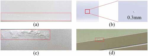
The data used in this paper are from the Tianchi aluminum surface defect dataset (Tianchi 2018). The image resolution is 2560 × 1920. Since there are many types of defects in the original dataset and most of them are defects of common size that are easy to detect, the low accuracy and low recall rate of defects of extreme size are masked in the evaluation of the results. Hence, we modify the original dataset by considering two representative types of defects, that is, those with the largest aspect ratios and smallest resolutions (scratches and spots), and use two types of typical defects (wrinkles and bumps) as controls. These training data are enhanced by flipping and rotating. Eventually, 1600 images are obtained. Each of these 1600 images is manually labeled. Sixty percent of the dataset is used as the training set, and the validation and test sets each account for 20%. Sample images of the four types of defects are shown in Figure 6.

Figure 6. Schematic of defects. (a) Scratches, (b) spots (size defects), (c) wrinkles, and (d) bumps.

Evaluation Indicators for Detection Results

The precision, recall, and mean average precision (mAP) are common indicators used to evaluate object detection performance. The formulas for the precision and recall are as follows:

(9) $Precision=\frac{TP}{TP+FP}$(9)

(10) $Recall=\frac{TP}{TP+FN}$(10)

where the true positive (TP) represents the number of defective areas detected as defects, the false positive (FP) represents the number of nondefective areas detected as defects, and false negative (FN) represents the number of defective areas detected as nondefective areas (Ren and Xue 2020; Wang et al. 2020). The precision-recall curve for a defect is plotted, and the area under the curve that lies above the x-axis is taken as the average precision (AP) of the defect. The mean of the AP values of all defects is taken as the mAP.

In this study, the AP and mAP are used to evaluate the detection results.

Analysis of Experimental Results

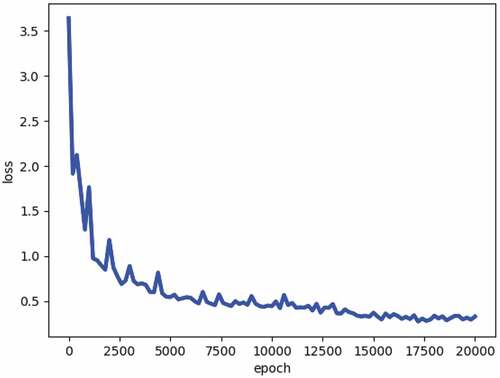
During training, the batch size is set to 16, the total number of training iterations is 20,000, and stochastic gradient descent (Theodoridis 2015) is used for optimization. The momentum factor μ is 0.9, and the weight attenuation coefficient ω is 0.0001. In addition, ResNet101 is used as the model backbone. The training loss curve is shown in Figure 7. The loss curve in the figure is obtained by sampling once every 200 epochs.

Figure 7. Loss curve.

Comparison of IoU Loss and GIoU Loss

To verify the effectiveness of the GIoU loss in place of the IoU loss, the GIoU loss and IoU loss are substituted into the original FCOS framework for comparison. The results are shown in Table 1. The AP values of all four types of defects (especially those of spots and bumps) evidently increase. The experimental results show that the use of GIoU loss can increase the mAP by 2.9%.

Table 1. Comparison of the IoU loss and GIoU loss (√ denotes that the AP was improved after introducing the GIoU loss).

Baseline	GIoU	GN	Improved center-ness	Self-adaptive	AP (%)
					Scratches	Spots	Wrinkles	Bumps
FCOS	˟	˟	˟	˟	50.2	69.7	79.3	74.1
FCOS	√	˟	˟	˟	52.9	74.4	80.5	77.0

Comparison of Batch Normalization and Group Normalization

For microdefects, such as spots in the dataset, the use of compressed images inevitably leads to the loss of defect information. Therefore, it is necessary to input the original size image into the network. In addition, the use of a smaller batch size for training results in batch normalization being inferior to group normalization. Based on the advanced FCOS model discussed in 3.3.1, we replace batch normalization with group normalization. The comparative experiment results are shown in Table 2. The AP of spot detection is significantly improved, the AP of the detection of other three types of defects is improved, and the overall mAP is increased by 1.5%.

Table 2. Comparison of the effects of batch normalization and group normalization.

Baseline	GIoU	GN	Improved center-ness	Self-adaptive	AP (%)
					Scratches	Spots	Wrinkles	Bumps
FCOS	√	˟	˟	˟	52.9	74.4	80.5	77.0
FCOS	√	√	˟	˟	53.8	78.0	80.9	78.2

Comparison Between the Improved Center-Ness and Original Center-Ness

In the dataset, most scratches are defects of extreme size that lie near the widest part of the image. The improved center-ness and the original center-ness are compared. The results show that after the center-ness is improved, the AP of scratch detection is increased by 4.4%. As shown in Table 3, the improved center-ness optimizes the detection of elongated defects by FCOS without affecting the detection of other types of defects, and the overall mAP is increased by 1.3%.

Table 3. Comparison of the experimental results of the improved center-ness and original center-ness.

Baseline	GIoU	GN	Improved center-ness	Self-adaptive	AP (%)
					Scratches	Spots	Wrinkles	Bumps
FCOS	√	√	˟	˟	53.8	78.0	80.9	78.2
FCOS	√	√	√	˟	58.2	78.7	80.7	78.5

Experimental Analysis of Self-Adaptive Center Sampling

The comparative experimental results of self-adaptive center sampling and center sampling are shown in Table 4. Since self-adaptive center sampling is also an improvement targeting elongated defects, it effectively improves the AP of scratch detection from 58.2% to 62.0%. The overall mAP increases from 74% to 75.4%.

Table 4. Analysis of experimental results for self-adaptive center sampling and center sampling.

Baseline	GIoU	GN	Improved center-ness	Self-adaptive	AP (%)
					Scratches	Spots	Wrinkles	Bumps
FCOS	√	√	√	˟	58.2	78.7	80.7	78.5
FCOS	√	√	√	√	62.0	80.2	81.1	78.3

Overall Analysis of Experimental Results

The experimental results are visualized in Figure 8. The results of the entire ablation experiment are presented in Table 5 and show that, based on the original FCOS framework, the performance for detecting defects of extreme size can be optimized for each improvement experiment and the accuracy of detection of normal-size defects can be improved to some extent. For ultra-elongated scratches, the AP can reach 62%, with an increase of 11.8%, while the AP of detecting microspots can even exceed 80%, with an increase of 10.5%. For the detection of wrinkles and bumps (defects of common size), the AP increases by 1.8% and 4.2%, respectively.

Figure 8. Visualization of the detection results, where defects 1 to 4 represent scratches, spots, wrinkles, and bumps, respectively.

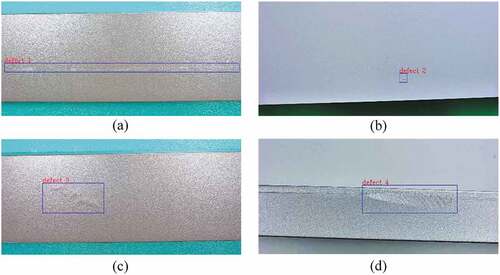
Table 5. Comparison of experimental results of the five-stage model.

Baseline	GIoU	GN	Improved center-ness	Self-adaptive	AP (%)
					Scratches	Spots	Wrinkles	Bumps
FCOS	˟	˟	˟	˟	50.2	69.7	79.3	74.1
FCOS	√	˟	˟	˟	52.9	74.4	80.5	77.0
FCOS	√	√	˟	˟	53.8	78.0	80.9	78.2
FCOS	√	√	√	˟	58.2	78.7	80.7	78.5
FCOS	√	√	√	√	62.0	80.2	81.1	79.7

Comparison of Advanced FCOS and Other Anchor-Based Methods

For the anchor-based methods, it is necessary to define the anchors based on the defects. Faster R-CNN defines nine anchors of fixed size. YOLOv3 and YOLOv5 obtain the appropriate anchors through clustering. YOLOv5x is the version with the strongest detection capability among YOLOv5 series. Figure 9 is a scatter plot of the defect size distribution in the aluminum-surface-defect dataset. In the figure, the sizes of the four types of defects are widely distributed: both the width and length follow a nearly random distribution in the interval (1, W), where W denotes the width of the input image. Neither the defined anchors nor the anchors obtained by clustering can be well fitted. In fact, the anchor-based methods generally rely on increasing the number of anchors to solve these problems, which seriously affects the detection efficiency and can even make the network difficult to train.

Figure 9. Scatter plot of size distribution of defects in the dataset.

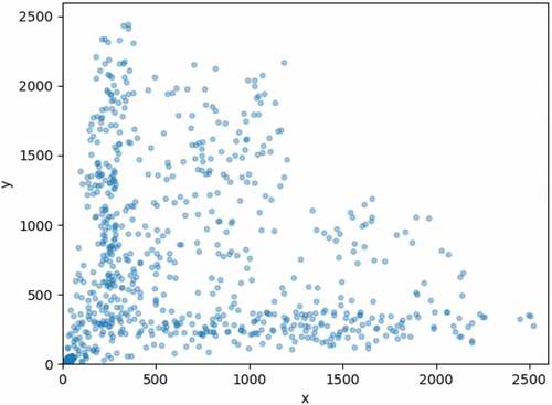
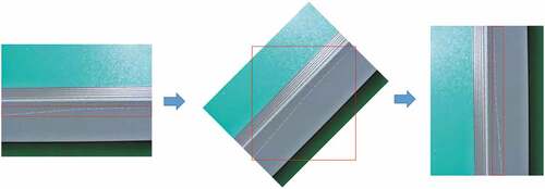
As shown in Figure 10, when the angle of an ultra-elongated defect is rotated from horizontal to 45° and 90°, the aspect ratio of the bounding box changes sharply, which corresponds to the overly large Euler distance between the two points in Figure 9. Consequently, the detection performance of the anchor-based methods drops. Therefore, the anchor-based methods are not suitable for the detection of defects of extreme size.

Figure 10. Schematic diagram of the change in the bounding box when the angle of an elongated defect changes.

Advanced FCOS and the anchor-based methods are compared on the test set. The AP (%) values of the detection of the four types of defects are shown in Table 6. Among these methods, Faster R-CNN also uses ResNet101 as the backbone and introduces the FPN structure. YOLOv3 uses DarkNet as the backbone. The hyperparameters for both YOLOv3 and YOLOv5x were set to default values proposed by its creators. The number of anchors in both models is set to the default value of 9. It can be seen that the mAP of our model for the detection of the four types of defects is significantly higher than that of Faster R-CNN, by 8.3%, and that of YOLOv5x, by 9.4%. If we look only at the two types of defects of extreme size, i.e., scratches and spots, the improvements are even more obvious. For example, the AP for spot detection using our model is higher than that of Faster R-CNN by 12.3% and that of YOLOv5x by 14.9%. The visualized examples of the scratch detection results of the four models are shown in Figure 11. The figure shows that the ranges detected by Faster R-CNN, YOLOv3 and YOLOv5x differ considerably from the actual values, resulting in lower AP values.

Figure 11. Comparison of the scratch detection results for (a) Faster R-CNN detection, (b) YOLOv3 detection, (c) YOLOv5x detection and (d) our model.

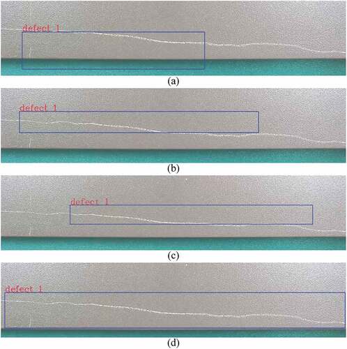
Table 6. Comparison of the AP values of the three models.

	Faster R-CNN	YOLOv3	YOLOv5x	Our model
Scratches	48.7	48.2	49.1	62.0
Spots	67.9	63.5	65.3	80.2
Wrinkles	77.9	75.7	77.6	81.1
Bumps	75.6	72.6	73.5	79.7
mAP	67.5	65.0	66.4	75.8

The detection speeds are compared in Table 7. YOLOv5x has a detection speed of approximately 28 f/s and the best real-time performance, whereas Faster R-CNN has a detection speed of approximately 0.8 f/s. The detection speed of the proposed method (6 f/s) lies between Faster R-CNN and YOLO methods, whereas the size of input image is approximately 28 times that of YOLOv3. The advanced FCOS method is suitable for real industrial detection.

Table 7. Comparison of the detection speeds of the three models.

	Faster R-CNN	YOLOv3	YOLOv5x	Our model
fps (f/s)	0.8	25	28	6

Conclusions

Ultra-elongated and ultra-fine defects are prone to be missed and false detection during manufacturing, in this study an advanced fully convolutional one-stage object detector is proposed to solve this problem. We improved the original FCOS framework, proposed center-ness and self-adaptive center sampling to prevent center suppression, and improved the regularization method and the loss function based on the defect characteristics. Experimental results show that the proposed method significantly improves the performance of the network in detecting defects of extreme size, including elongated defects and microdefects, without affecting the detection of normal-size defects. The proposed method outperforms Faster R-CNN, YOLOv3 and YOLOv5x on the aluminum-surface-defect dataset. In addition, the proposed method can detect large images (>2Kx2K) at 6 f/s, which meets the requirements of real-time industrial detection.

Disclosure statement

No potential conflict of interest was reported by the author(s).

Additional information

Funding

The work was supported by the Chinese National Funding of Social Sciences [51775214].

References

- Bae-Keun, K., W. Jong-Seob, and D.-J. Kang. 2015. Fast defect detection for various types of surfaces using random forest with vov features. International Journal of Precision Engineering and Manufacturing 16 (5):965–3142. doi:10.1007/s12541-015-0125-y.
- Bauer, S., S. Köhler, K. Doll, et al. 2010. FPGA-GPU architecture for kernel SVM pedestrian detection. IEEE Computer Society Conference on Computer Vision Pattern Recognition Workshops (CVPRW): 61–68. doi: 10.1109/CVPRW.2010.5543772.
- Chen, D.-S., and Z.-K. Liu. 2007. Generalized Haar-like features for fast face detection. International Conference on Machine learning Cyberne, Hong Kong: 2131–35. doi: 10.1109/ICMLC.2007.4370496.
- Duje, M., P. Luka, S. Marko, B. Marko, and L. Sven. 2022. DefectDet: A deep learning architecture for detection of defects with extreme aspect ratios in ultrasonic images. Neurocomputing 473:107–15. doi:10.1016/j.neucom.2021.12.008.
- Gan, G., and J. Cheng 2011. Pedestrian detection based on HOG-LBP feature. International Conference and Computing Intelligence Security, Hainan: 1184–87. doi:10.1109/CIS.2011.262.
- Girshick, R., and Fast R-CNN2015. arXiv e-prints 1440–48. 10.48550/arXiv.1504.08083.
- Girshick, R.-B., J. Donahue, T. Darrell, et al. 2014. Rich feature hierarchies for accurate object detection and semantic segmentation. IEEE Conference on Computer Vision and Pattern Recognition, Columbus, USA: 580–87. doi: 10.1109/CVPR.2014.81.
- Han, P., and J.-M. Liao. 2009. Face detection based on adaboost. International Conference Apperceiving Computing and Intelligence Analysis, Chengdu: 337–40. doi: 10.1109/ICACIA.2009.5361085.
- He, K., X. Zhang, S. Ren, et al. 2016. Deep residual learning for image recognition. IEEE Conference on Computer Vision & Pattern Recognition, Las Vegas, NV, USA. doi: 10.1109/CVPR.2016.90.
- Huang, L., Y. Yang, Y. Deng, et al. 2015. DenseBox: Unifying landmark localization with end to end object detection. Computer Science. doi:10.48550/arXiv.1509.04874.
- Ioffe, S., and C. Szegedy. 2015. BaTch normalization: accelerating deep network training by reducing internal covariate shift. 32th International Conference on Machine Learning: 448–56. doi: 10.48550/arXiv:1502.03167.
- Ji, W.-X., M. Du, W. Peng, et al. 2019. Research on gear appearance defect recognition based on improved faster R-CNN. Journal of System Simulation 31 (11):2198–205. doi:10.16182/j.issn1004731x.joss.19-0545.
- Krizhevsky, A., I. Sutskever, and G.-E. Hinton. 2017. ImageNet classification with deep convolutional neural networks. Communications of the ACM 60 (6):84–90. doi:10.1145/3065386.
- Lin, T.-Y., P. Dollar, R. Girshick, et al. 2017. Feature pyramid networks for object detection. IEEE Conference on Computer Vision and Pattern Recognition. doi: 10.48550/arXiv.1612.03144.
- Lin, T.-Y., P. Goyal, R. Girshick, et al. 2017. Focal loss for dense object detection. IEEE Transactions on Pattern Analysis & Machine Intelligence 2980–88. doi:10.1109/TPAMI.2018.2858826.
- Liu, W., D. Anguelov, D. Erhan, et al. 2016. SSD: Single shot multibox detector. European Conference on Computer Vision. doi: 10.1007/978-3-319-46448-0_2.
- Liu, H.-B., and G.-W. Kang. 2005. Surface defects inspection of cold rolled strips based on neural network. Journal of Image and Graphics 10 (10):109–12. doi:10.11834/jig.2005010236.
- Redmon, J., S. Divvala, R. Girshick, et al. 2016. You only look once: Unified, real-time object detection. IEEE Conference on Computer Vision and Pattern Recognition, Las Vegas: 779–88. doi:10.1109/CVPR.2016.91.
- Redmon, J., and A. Farhadi. 2017. YOLO9000: Better, Faster, stronger. IEEE Conference on Computer Vision and Pattern Recognition, Honolulu: 6517–25. doi: 10.1109/CVPR.2017.690.
- Redmon, J., and A. Farhadi. 2018. Yolov3: An incremental improvement. arXiv e-prints. doi:10.48550/arXiv.1804.02767.
- Ren, S.-Q., K.-M. He, R. Girshick, et al. 2015. Faster R-CNN: Towards real-time object detection with region proposal networks. IEEE Transactions on Pattern Analysis and Machine Intelligence 39 (6):91–99. doi:10.1109/TPAMI.2016.2577031.
- Ren, F.-J., and S.-Y. Xue. 2020. Intention detection based on Siamese neural network with triplet loss. IEEE Access 8:82242–54. doi:10.1109/ACCESS.2020.2991484.
- Rezatofighi, H., N. Tsoi, J.-Y. Gwak, et al. 2019. GeneralIzed intersection over union: a metric and a loss for bounding box regression. IEEE Conference on Computer Vision and Pattern Recognition: 658–66. doi: 10.1109/CVPR.2019.00075.
- Shelhamer, E., J. Long, and T. Darrell. 2017. Fully convolutional networks for semantic segmentation. IEEE Transactions on Pattern Analysis and Machine Intelligence 39 (4):640–51. doi:10.1109/CVPR.2015.7298965.
- Simonyan, K., and A. Zisserman. 2014. VeRy deep convolutional networks for large-scale image recognition. Computer Science. doi:10.48550/arXiv.1409.1556.
- Theodoridis, S. 2015. Stochastic gradient descent. Machine Learning 161–231. doi:10.1016/B978-0-12-801522-3.00005-7.
- Tian, Z., C. Shen, H. Chen, et al. 2019. FCOS: Fully convolutional one-stage object detection. IEEE/CVF International Conference on Computer Vision. doi: 10.48550/arXiv.1904.01355.
- Tian, Z., C.-H. Shen, H. Chen, and T. He. 2020. FCOS: A simple and strong anchor-free object detector. IEEE Transactions on Pattern Analysis and Machine Intelligence 1. doi:10.1109/TPAMI.2020.3032166.
- Tianchi. 2018. https://tianchi.aliyun.com/competition/entrance/231682/information.
- Wang, Z., Y. Jia, H. Huang, et al. 2008. Pedestrian detection using Boosted HOG features. Proceedings of the IEEE Conference Intelligence and Transport Systems, Beijing: 1155–60. doi:10.1109/ITSC.2008.4732553.
- Wang, J., Q. Li, J. Gan, H. Yu, and X. Yang. 2020. Surface defect detection via entity sparsity pursuit with intrinsic priors. IEEE Transactions on Industrial Informatics 16 (1):141–50. doi:10.1109/TII.2019.2917522.
- Wang, H. Y., J. Zhang, Y. Tian, et al. 2018. A simple guidance template-based defect detection method for strip steel surfaces. IEEE Transactions on Industrial Informatics. 15(5):2798–809. doi:10.1109/TII.2018.2887145.
- Wu, Y.-X., and K.-M. He. 2018. Group Normalization. International Journal of Computer Vision. doi:10.1007/s11263-019-01198-w.
- Yu, J., Y. Jiang, Z. Wang, et al. 2016. Unitbox: An advanced object detection network. ACM on Multimedia Conference: 516–20. doi: 10.1145/2964284.2967274.
- Zhang, X., and D.-J. Huang. 2020. Defect detection on aluminum surfaces based on deep learning. Journal of East China Normal University (Natural Science) 06:105–14. doi:10.3969/j.issn.1000-5641.201921021.
- Zhou, X.-Y., D.-Q. Wang, and P. Krahenbühl. 2019. Objects as Points. arXiv e-prints. doi:10.48550/arXiv.1904.07850.