LifeGuard: An Improvement of Actor-Critic Model with Collision Predictor in Autonomous UAV Navigation

ABSTRACT

The needs for autonomous unmanned aerial vehicle navigation (AUN) have been emerging for recent years due to the growth of the logistic industry and the need for social distancing during the pandemic. There have been different methods trying to overcome the AUN task, and most of them have focused on deep reinforcement learning (DRL). But the results were still far from satisfactory, and even if the result was good, the environment was usually too trivial and simple. We report in this paper one of the causes of low success rate for AUN in our previous work, which is the apprehensive behavior of agents. After numerous episodes of training, when the agent faces risky scenes, it often moves back and forth repeatedly until running out of the limited steps. Hence, in this paper, we propose a new role, LifeGuard, into the popular DRL model, Actor-Critic, to tackle the apprehensive behavior and expect a better success rate. In addition, we developed a pilot method of unsupervised classification for sequential data to further enhance our reward function from previous work, augmentative backward reward function. The experimental results demonstrated that the proposed method can eliminate the apprehensive behavior and gain higher success rates than the state-of-the-art method, FORK, with lesser effort.

Introduction

Unmanned aerial vehicle (UAV), commonly referred to as drones, has gradually played a prominent role in various applications due to its high mobility compared to ground traffic congestion. Nowadays, its main target has been where it is difficult (or risky) for humans to reach (Jain et al. 2018; Sudhakar et al. 2020). It is a disappointment that using UAVs on regular tasks such as an errand service still did not receive as much attention as it should have. The hindrance may be due to the fact that the reliable UAV navigation methods are still manual or semi-automated (Castaño et al. 2019; Hawary and Razak 2018). However, it means that the manpower is still required throughout the entire runtime, and it does not reduce the cost. The autonomous UAV navigation (AUN) development has a long history but is just impelled lately by two main factors. First, there is a need for remote surrogates, in which manpower can be reduced for various industries, such as transportation, surveillance, and resource exploration, and can help avoid physical contact during the pandemic. The second factor is the incessant development of deep learning that brings AUN closer to real-world adoption. In recent years, there are efforts put into autonomous navigation and could be widely divided into two approaches: 1) path planning approach and 2) reinforcement learning (RL) approach. The instances of path planning approach are as follows: Youn et al. (2020) proposed a UAV navigation technique, which combines the advantages of variant rapidly random trees (RRT) algorithms with the help of error state Kalman filter integration. Their technique reduces redundancy on random node generation from the conventional path planning. This technique compares neighboring node costs (RRT-Smart) as well as dynamic directional path lengths (RRT*-GD) to better prevent unnecessary node generations. Elmokadem and Savkin (2021) proposed the AUN method also with the RRT algorithm called RRT-connect. This method generates the trajectory path of the UAV by converging the two trees toward each other from the start and goal points. In order to avoid collision, they use reactive control law, which is designed to make the UAV move around the obstacle until it met the safe condition. After that, the UAV came back along the previous planned path. Though this approach does not need any prior knowledge about the environment, it needs some expertise knowledge on structuring the obstacle avoidance procedure, which is hard to be sufficiently flexible for a realistic environment. In addition, these two approaches are able to afford only discrete spaces, so the movement is rigid and not of full potential. Regarding the instances of RL approach, Guo et al. (2020) indicated that even though the recent deep reinforcement learning (DRL) methods earned quite good results, those cannot converge to satisfied points in high-dimensional state-action spaces task like AUN. So, they decided to bring the divide-and-conquer strategy to this complex task. The AUN task will be organized into three parts including collision avoidance, goal approach, and decision. These parts are represented as recurrent neural networks: avoid network, acquire network, and packed network. Avoid and acquire networks are responsible for offering a packed network a next action; then the packed network decides which is the appropriate action for the current state, avoiding the obstacle or approaching the goal. If the decision is wrong, the packed network will receive a punishment as a negative reward. Their result indicated that this model improves the success rate, collision rate, and velocity when compared with variant deep Q networks. Furthermore, there was a cooperation between fully autonomous aerial systems (FAAS) and mobile edge computing (MEC) to navigate UAV for crowd surveillance purposes. Apostolopoulos, Torres, and Eleni Tsiropoulou (2019) introduced the framework to serve the purpose and mainly addressed the data offloading problem. The devices need to satisfy their individual quality of service (QOS) and also regarding the energy consumption, and they overcame these problems by using an on-policy RL algorithm named state-action-reward-state-action (SARSA) (Rummery and Niranjan 1994) and satisfaction equilibrium concept. All results from both path planning-based and RL-based methods show that they are still dissatisfied for the real-world adoption but be able to support more realistic conditions and higher state-action spaces.

Now, the most promising method seems to be the DRL method due to the fact that there are several of them combining deterministic and stochastic techniques to achieve high continuous spaces in the motion control and decision-making tasks, and the results were quite good (Guo et al. 2020). This field, DRL, has been dominated by an actor-critic model. The most widely known method of this model was deep deterministic policy gradient (DDPG) (Lillicrap et al. 2015); it combines Q-learning with policy gradient to let the model allow continuous space. Subsequently, the two descendants of DDPG called twin delayed DDPG (TD3) (Fujimoto, van Hoof, and Meger 2018) and soft actor critic (SAC) (Haarnoja et al. 2018a, 2018b) had arisen recurrently. It achieved promising performance in many tasks (Haarnoja et al. 2018; Zhang, Li, and Li 2020) and became the state-of-the-art methods. These two methods focus on the same thing, which is Q-value overestimation, the main flaw of DDPG, and also leverage the same thing, the target policy smoothing, to alleviate the overestimation. Despite many brilliant proofs of two state-of-the-art methods, TD3 and SAC, which are almost maximum scores for many tasks (Fujimoto, van Hoof, and Meger 2018; Haarnoja et al. 2018), there are still tasks where both methods have not achieved yet or been very time consuming (Wei and Ying 2020). Recently, the addition of both methods has emerged to improve the policy. Zhang et al. (2020) addressed the slow convergence rate in TD3 by adapting some prior knowledge in the form of alternative action. This action is generated from error and three parameters, which are tuned to suit the environment. This action and the action from the actor are estimated by their Q values to decide which one is better. This alternative action helps improve training speed and learning stability for TD3. Wei and Ying (2020) proposed the additional method named forward-looking actor (FORK); it tries to learn the system model (model-based RL) but not quite deterministic or stochastic policy optimization, which is mainly based on the model. It is just forecasting the next state and the reward after executing the action at given states and letting the forecasts participate in the policy adjustment. Hence, any actor-critic methods added FORK are still model-free. This addition, FORK, with some heuristic changes could solve a severely difficult task, BipedalWalkerHardcore, within 4 hours by only using a single GPU. These are evidence that having the addition helps the actor learn optimal policy easier, and the results often go through the roof.

Despite many efforts to improve AUN, the main problems still exist (Lu et al. 2018; Maciel-Pearson et al. 2019). In recent work on AUN, their success rate that the agent can reach to the goal was moderate even in low action space, simplified static environments, and unrealistic sensors (Elmokadem and Savkin 2021; Zijian et al. 2020). Furthermore, the collision rate was still worrisome that it should not happen in real-world adoption (Zonneveld 2018). Simultaneous localization and mapping (SLAM) for UAV in precise tasks like delivering has also been a difficult challenge (Sadeghzadeh-Nokhodberiz et al. 2021). In sum, the AUN’s problems in many aspects are just alleviated but not wiped out. From our previous work (Chansuparp and Jitkajornwanich 2022), we found that certain AUN‘s problems were caused by traditional reward (TR) function, which has been in common use for many navigation tasks (Zhang et al. 2020; Zijian et al. 2020). This function will return a large constant positive value as a reward when the agent reaches the goal to encourage this behavior and return a constant negative value as a punishment when the agent collides with environment objects to dissuade. We set the hypothesis that this reward mechanism causes the bias on the scene that looks like one at the goal; it will suit only the simple environment, which seldom found the look like goal scenes. Our previous experimental results empirically showed that changing the chunk of reward given to a last transition to reward dispersion proportional to each transition’s participation could greatly improve the performance. But, after observation in the rear episodes of training, we found that certain problems in AUN are tied together. It is rather simple to reduce collision rate by increasing the punishment, but the consequence is that the success rate will be low since the agent will be apprehensive when it faces risky scenes. This makes the agent move back and forth before a risky scene and leads to running out of quota steps. Apparently, it is a trade-off.

Hence, in this work, we propose two new things to solve the agent’s apprehensive behavior and to improve the performance for navigation tasks. First, the LifeGuard (LG) is a new role proposed into an actor-critic model. The LifeGuard is responsible for evaluating whether the given state-action pairs will lead to the collision or not. The forecast from LifeGuard is used to adjust the action selection process in actor networks. For many tasks, more risk means more reward, and a very thin difference in action can cause the reward to be different as night and day. It is hard to recognize the existence of this dividing line while simultaneously learning the way to earn more reward, especially in high state-action spaces. In short, the LifeGuard helps the actor and critic to recognize this line much faster. In addition, we also propose a pilot study on unlabeled sequential data classification with all positive Siamese auto encoder (PSAE) to improve our previous reward function, augmentative backward reward function (ABR) (Chansuparp and Jitkajornwanich 2022). The performance of our method is measured on AUN task and BipedalWalkerHardcore-gym, the test bed for RL algorithms, to confirm that the method is robust. All our experiments are conducted on the realistic simulation due to the fact that the collision rate of even the state-of-the-art method is still concerned and the negligible collision may cause inability to the UAV. If the experiments are conducted with real devices, the implementation cost would have been around 5,100 USD in which 1,100 USD is estimated for the quadrotor UAV and 4,000 USD is estimated for VLP-16 LiDAR sensor.

The video of our test can be seen here: https://youtu.be/OkNSfLbknIE.

Background

AUN task physically consists of two things: an agent and environment. The aim is also rather simple, which is to navigate the UAV to the goal point without collision. Even so, there are studies that point out that to accomplish navigation tasks in a complex and dynamic environment, using the state-of-the-art methods in deep RL like TD3 and SAC alone is insufficient (Qiu et al. 2020; Wei and Ying 2020). The recent results of AUN in a realistic environment and a realistic agent are around 60% (Chansuparp and Jitkajornwanich 2022; Zijian et al. 2020). In this section, we describe the components related to the current AUN problem.

UAV Kinematics

Figure 1. Position and Euler angles of UAV in a 3D environment.

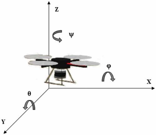
UAV is able to move freely in six degrees of freedom (6DoF) (as shown in Figure 1) and so to control its motion requires six parameters including three linear velocities and three angular velocities ($l_x,l_y,l_z,a_x,a_y,a_z$). The translation ($\stackrel{\dot{y}}{x,},\dot{z}$) and rotation ($Roll\dot{\phi },Pitch\dot{\theta },Yaw\dot{\psi }$) of UAV on three-dimensional cartesian coordinate space can be done by this:

(1) $\left[\begin{array}{c}\begin{array}{c}\dot{x}\\ \dot{y}\\ \dot{z}\end{array}\\ \begin{array}{c}\dot{\phi }\\ \dot{\theta }\\ \dot{\psi }\end{array}\end{array}\right]=\left[\begin{array}{c}\begin{array}{c}{l}_x\\ l_y\\ l_z\end{array}\\ \begin{array}{c}0\\ 0\\ 0\end{array}\end{array}\right]\left[\begin{array}{c}\begin{array}{c}cos\theta cos\psi \\ \mathrm{s}\mathrm{i}\mathrm{n}\theta cos\psi \\ \mathrm{s}\mathrm{i}\mathrm{n}\psi \end{array}\\ \begin{array}{c}0\\ 0\\ 0\end{array}\end{array}\right]+\left[\begin{array}{c}\begin{array}{c}0\\ 0\\ 0\end{array}\\ \begin{array}{c}{a}_x\\ a_y\\ a_z\end{array}\end{array}\right]\left[\begin{array}{c}\begin{array}{c}0\\ 0\\ 0\end{array}\\ \begin{array}{c}1\\ 1\\ 1\end{array}\end{array}\right]$(1)

In a realistic environment, the UAV motion is resisted by gravitational and aerodynamic forces, which are given by Chansuparp and Jitkajornwanich (2022). But with disappointment, almost all recent works on AUN do not take these external forces into account and determine the action space with merely two or three dimensions, which are only linear velocities. In previous and this work, we let the UAV move in four dimensions ($l_x,l_y,l_z,a_z$) and underneath the external forces. The reason we put $a_z$ in is that almost all applications demand the UAV to always stay toward the goal since many devices equipped on UAV such as cameras and sensors have limited field of view (FOV).

Deep Reinforcement Learning

The basic aim of RL algorithms is to learn the policy, which can manage the agent to gain maximum cumulative reward from interacting with the environment. The interaction transition between the agent and the environment is often structured in form of Markov decision process (Bellman 1957), which is represented as tuple $\left(S,A,P,R,\gamma \right)$. $S$ is a set of possible world states. $A$ is a set of possible actions. $P$ is a probability of executing action $A$ at state $S$ to reach next state $s$ (where $a\in A$ and $s,s\in S$). $R$ is a reward received by transmitting the agent from $s\to s$. $\gamma \in \left[0,1\right]$a discount factor determining how important the future reward is. At each time step $t$ (a discrete value), the action $a_t$ is generated based on policy $\mu \left(s_t\right)$. After executing $a_t$, the agent reaches to state $s_{t+1}$ and receive reward $r_t$. As aforementioned, the state-of-the-art model to learn optimal policy ${\mu }^{\ast }$ in continuous spaces still has been the actor critic model. We consider the actor and critic in DDPG. The actor selects an action expected to give high reward for given state $s_t$ and the critic tell the actor how good the selected action is (value function $Q\left(s,a\right)$). Both the actor and critic have a time-delayed network of itself to alleviate the instability issue of Q-learning in deep neural networks (DNNs). The main and time-delayed networks are called eval-net and target-net, respectively. To update the parameters in actor ${\theta }^{\mu }$, transitions are sampled in Monte Carlo fashion to approximate the Q values and its parameters. The actor (policy function) is differentiable; the chain rule can be applied as follows:

(2) ${\mathrm{\nabla }}_{{\theta }^{\mu }}J\left({\theta }^{\mu }\right)=\frac{1}{N}{\sum }_{i=1}^N{\mathrm{\nabla }}_{a}Q(s,a|{\theta }^Q{)}_{a=\mu \left(s_i\right)}{\mathrm{\nabla }}_{{\theta }^{\mu }}\mu (s|{\theta }^{\mu })$(2)

$N$ denotes batch size.

In terms of the critic, the parameters ${\theta }^Q$ are updated by minimizing this loss function.

(3) $L_c\left({\theta }^Q\right)=\frac{1}{N}{\sum }_{i=1}^N((y_i-Q(s_i,a_i|{\theta }^Q){)}^2{y}_i=r\left(s_i,a_i\right)\gamma Q{ }^{\mathrm{\prime }}(s_{i+1},\mu { }^{\mathrm{\prime }}(s_{i+1}|{\theta }^{\mu { }^{\mathrm{\prime }}})|{\theta }^{Q{ }^{\mathrm{\prime }}})$(3)

$\mu { }^{\mathrm{\prime }},Q{ }^{\mathrm{\prime }}$ denote the parameters of actors and critics in target-nets.

The parameters of the target-net are soft-updated by eval-net at some small intervals. Nonetheless, many works (Fujimoto, van Hoof, and Meger 2018; Meng, Gorbet, and Kulić 2021) indicated that DDPG overestimates the Q-value and then the policy leads to significant failure. There are methods built on DDPG addressing this problem. We focus on one among them, twin delayed DDPG (TD3). Fujimoto, van Hoof, and Meger (2018) proposed three tricks to address this problem: First, double the Q-function and use the smaller one to always be modest. Second, update the policy and target-nets less frequently than Q-function to let it exploit a lower error Q-value. Third, add clipped noise to the target action to reduce variance of target values. The full detail of TD3 was given by Chansuparp and Jitkajornwanich (2022).

Forward-Looking Actor

Generally, the actor improves the policy with the value of the critic provided. The general loss function of this improvement is as follows:

(4) $L_o\left(\theta \right)=-Q(s_t,\mu (s_t|\theta ))$(4)

Wei and Ying (2020) proposed the foresightful policy improvement algorithm. It may be better if the action selection regards not only a current reward but also future benefits. To do so, they add two neural networks, which are in charge of learning the system model and the reward function, called system-net and reward-net, respectively. The system-net is learned to forecast a next state $s_{t+1}$ of any given state-action pair ($F(s_t,a_t|{\theta }^F)$). The reward-net forecasts a reward, which will receive after executing state-action pair ($R(s_t,a_t|{\theta }^R)$). Their loss function of the actor network could be formulated as follows:

(5) $L_{aF}\left({\theta }^{\mu }\right)=-Q\left(s_t,\mu \left(s_t|{\theta }^{\mu }\right)|{\theta }^Q\right)-R\left(s_t,\mu \left(s_t|{\theta }^{\mu }\right)|{\theta }^R\right)-\gamma R\left({\tilde{s}}_{t+1},\mu \left({\tilde{s}}_{t+1}|{\theta }^{\mu }\right)|{\theta }^R\right)-{\gamma }^{2}Q({\tilde{s}}_{t+2},\mu \left({\tilde{s}}_{t+2}|{\theta }^{\mu }\right)|{\theta }^Q)$(5)

where ${\tilde{s}}_{t+1},{\tilde{s}}_{t+2}$ denote future states of $s_t$ forecasted from system-net.

Their experiments on the open AI gym showed that adding FORK to the state-of-the-art model-free RL algorithms helps boost the performance in terms of both cumulative reward and time complexity. FORK outperforms other model-based RL algorithms.

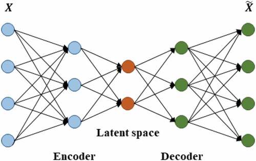
Autoencoder

The autoencoder, as the name suggests, is a neural-network-based feature extraction method that does not need any supervised knowledge. The network consists of three components: First, an encoder, a module which compresses input data into a small compressed representation (features of data). Second, a bottleneck, the most compressed representation of input data is stored here and is thereby the essence of the network. Third, a decoder, a module that decompresses a compressed representation and reconstructs it back to the almost original input data. The network expects output to be the same or similar to input for ensuring that there is still vital information in bottleneck (or latent space). The architecture of the whole network can be seen in Figure 2.

Figure 2. Autoencoder network.

There are various improvements on autoencoder such as denoising autoencoder (Vincent et al. 2008), which add noise on the input to make the network more robust against discrepancy, sparse autoencoder (Ng 2011), which regularize autoencoder by sparsity constraint, and so on. In addition, there is a combination between autoencoder and Siamese network model with triplet loss (Schneider et al. 2019) to exploit the good representation in latent space and distance-based classification ability. The triplet loss function helps the features of data in the same class get closer than those from other classes. The function can be defined as follows:

(6) $L_T=max\left(d\left(a,p\right)-d\left(a,n\right)+m,0\right)$(6)

where $d$ denotes a distance matrix function. $a,p$ denote an anchor sample and sample in the same class as anchor (positive sample). $n$ denotes the different class, negative sample. $m$ denotes some margin value.

Augmentative Backward Reward Function

Figure 3. Workflow of augmentative backward reward function.

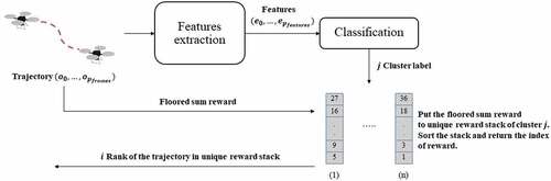
In our previous work, we proved the severe problem of TR function in navigation tasks and proposed the new reward function, which is more rational, called ABR. Adding an extra reward to stimulate the agent to reach the goal can be a double-edged sword; it will negatively affect the agent instead if the goal reward dispensation is irrational. ABR adds an extra reward to all positive-rewards trajectories in success episodes. The trajectory means the sequence of observations, which the agent receives from the environment at each step $\left(o_1,\dots ,o_l\right)$, where $l$ denotes a constant value of sequence length. The trajectories are features extracted in an unsupervised manner by convolution-based one-shot learning, and we can classify them based on their cosine similarity to each other. Each cluster of trajectories has its own unique stack of floored sum of rewards in trajectory to measure the level of contribution for each trajectory. The workflow of ABR was shown in Figure 3 and the extra reward can be calculated as follows:

(7) $r_e=i\times p_{exR}$(7)

where $i$ denotes the rank in unique stack of floored sum and $p_{exR}$ denotes hyper-parameter.

And, the rewards for collided and other cases can be defined as follows:

$R\left(s,a\right)=\left\{\begin{array}{c}{r}_{colluded}(ifcollided)\\ w_1\left(D_{pre}-D_{cur}\right)+w_2\left(1-\left(\left(\left(z-PapproAlt\right)\right)/PapproAlt\right)\right)+\\ w_3\left(1-\left(v_h/180\right)\right)+w_4\left(1-\left(v_g/180\right)\right)(ifnotcollidedandnot\mathrm{r}\mathrm{e}\mathrm{a}\mathrm{c}\mathrm{h}\mathrm{e}\mathrm{d}\mathrm{t}\mathrm{h}\mathrm{e}\mathrm{g}\mathrm{o}\mathrm{a}\mathrm{l})\end{array}\right.$

(8) $V_h=\left\{\begin{array}{c}360-h(ifh>180)\\ h\end{array}\right.V_g=\left\{\begin{array}{c}360-g(ifg>180)\\ g\end{array}\right.$(8)

where $D_{pre},D_{cur}$ denote the previous and current Euclidean distances between the agent and goal, respectively, $z$ denotes altitude of UAV, $h,g$ denote angles of the UAV’s head and position to goal, respectively, $p_{approAlt}$ denotes appropriate altitude or flight level, and $w_{1-4}$ denote weight parameters.

Methodology

Unsupervised Trajectories Classification with All Positive Siamese Autoencoder

As mentioned in the section ‘Autoencoder’, Siamese model with triplet loss helps the features of data in the same class get close to each other and the features in different classes get apart such that it is much favorable for classification. But, it is the case that the positive and negative samples are known. If you consider denoising techniques to at least make the features robust against discrepancy, then the input data need to be distorted, and unlike the image data, this will quite change the meaning of trajectory data. With all these limitations, unsupervised trajectories classification has been arduous and also hard to concretely measure the accuracy. Hence, we propose a pilot study on unsupervised sequential data classification, which adapts the idea of Siamese autoencoder with triplet loss. In the absence of positive samples for a given trajectory, we assume that the past and future states $\left(s_{t-1},s_{t+1}\right)$ are approximately similar to the state $s_t$. In other words, we use adjacent states as surrogates of positive samples in triplet loss. To allow our autoencoder to be resilient for both aspects, the past and future, the Siamese-triplet model was adopted for encoding. The architecture of our PSAE is illustrated in Figure 4.

Figure 4. Network architecture of all positive Siamese autoencoder.

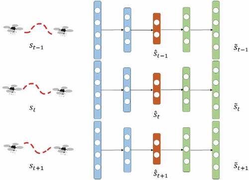
Our Siamese network consists of three identical sub-networks, which have the same architecture and shared parameters. The network receives $\left(s_{t-1},s_{t+1}\right)$ as two positive inputs and $s_t$ as an anchor input. The network returns reconstructed outputs $\tilde{s}$, which is expected to be similar to its own input $s$ according to autoencoder theory, and the features $\hat{s}$ in latent space (narrowest layer), which is expected to be close to the anchor’s features in terms of distance according to the triplet loss. So, our loss function is designed to minimize the mean squared error (MSE) between the input and output and to maximize the cosine similarities of the features pairs of the anchor with positives.

(9) $L_{PSAE}=p_{wae}{\sum }_{i=-1}^1{\left|\left|s_i-{\tilde{s}}_i\right|\right|}_2^2-\left(1-p_{wae}\right)\sum _{j=-1,1}coss\left({\hat{s}}_0,{\hat{s}}_j\right)$(9)

where $p_{wae}$ denotes the level of tradeoff between two terms and $coss$ denotes cosine similarity function.

In terms of classification, all the features $\hat{s}$ in buffer are clustered by the K-mean algorithm. The $k$ number is determined by the elbow method, the classical method, which has been popular for unsupervised clustering (Liu and Deng 2021; Shi et al. 2021). The elbow method finds the optimal $k$ number by iteratively calculating sum square error (SSE), the sum of average Euclidean distances between each data point and its centroid, and then picking the point where SSE is starting to stable, the graph’s part, which looks like an elbow.

(10) $SSE={\sum }_{k=1}^K{\sum }_{x\in C_k}{\left|\left|x-C_k\right|\right|}_2^2$(10)

where $K$ denotes maximum cluster number and $C$ denotes the centroid of the cluster.

In the context of high-dimensional state space, there are abundance of trajectory patterns and so we increase $k$ with some constant steps. After finding the optimal $k$, each state in buffer can be determined from its cluster label. These pairs of features and labels are used as training sets for the classifier. At the end, we replaced the one-shot classification in ABR with the PSAE classification and named it ABR+.

Actor-Critic-LifeGuard

This new role, LG, was inspired by the proof of FORK that the supplementary forecast can significantly improve the policy training. After testing FORK on AUN, we found that the loss values of system-net during the training fluctuate dramatically. This can imply that it is unaffordable to precisely forecast the future states in high-dimensional state-action spaces. Consequently, we aimed to develop the actor assistant, which is low sophistication. The LG is simply a binary classifier, which forecasts whether the agent will collide or not if it takes an action $a_k$ at state $s_k$. We adopt stochastic gradient descent (SGD) algorithm for learning the classifier since its linear complexity and scaling capability make the computation still fast even with huge and high-dimensional data (Mittal, Gaurav, and Sekhar Roy 2015). Let $\left(x_n,y_n\right)$be a set of training samples, $x\in R^m$ be features (the last observation in state) and $y\in \left\{1,0\right\}$ be label (collided, not). Please note that the SGD is sensitive to feature scaling, and all attributes in features should be scaled to (0,1). The output of the SGD classification can be got by:

(11) $c\left(x\right)=w^{T}x+j$(11)

where $w\in R^m$ denotes model parameters and $j\in R$ denotes intercept.

$w$ is found by minimizing the regularized training error with this cost function:

(12) $E\left(w,j\right)=\frac{1}{n}{\sum }_{i=1}^{n}L\left(y_i,c\left(x_i\right)\right)+\alpha R\left(w\right)$(12)

where $R$ denotes regularization term, the L2 norm, and $\alpha$ denotes a regularisation hyper-parameter.

For L, it denotes the loss function, and in this work, we adopted the logistic regression loss.

(13) $L\left(y_i,c\left(x_i\right)\right)=log\left(1+exp\left(-y_{i}c\left(x_i\right)\right)\right)$(13)

At each update time step, one training sample is taken, and the model parameters are updated according to this rule:

(14) $w\leftarrow w-lr\left[\alpha \frac{dR\left(w\right)}{dw}+\frac{dL\left(w^T{x}_i+j,y_i\right)}{dw}\right]l{r}^{\left(t\right)}=\frac{1}{\alpha \left(t_0+t\right)}$(14)

where $lr,t_0$ denote learning rate and initial time, respectively.

After training the LG for a while, the collision forecast is used to improve the policy (Actor) as follows:

(15) $L_{aL}\left({\theta }^{\mu }\right)=-\left(Q\left(s_t,\mu \left({\theta }^{\mu }\right)|{\theta }^Q\right)-c\left(o_t+\mu \left({\theta }^{\mu }\right)\right)p_{cp}\right)$(15)

where $o$ denotes the last observation in state $s$, and $p_{cp}$ denotes the hyperparameter controlling the diminishing of Q value.

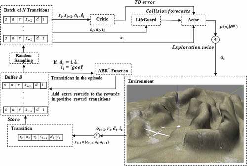
AUN with TD3-LG and ABR+

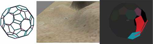
In this section, we describe the workflow of the proposed method as illustrated in Figure 6. There are some pre-processes that have to be declared before going to the policy learning process. In a realistic navigation setting, the agent’s perception is usually represented with a point cloud, which contains abundant points in space; around a few hundred thousand points, it cannot be directly used as an input for the learning process. Hence, all experiments involved with UAV in this work proceeded under point cloud simplification with truncated icosahedron structure, which was proposed in our previous work. This soccer-ball-shaped structure programmatically covers the agent to screen only the cloud points it needs to be careful of; then it turns the point cloud into 32 points according to the number of the structure’s sides as illustrated in Figure 5. The radius of this ball refers to the safe flying distance $p_{radius}$. For this work, the observation consists of 32 cloud points $\left(f_{1-32}\right)$, the altitude of UAV $\left(z\right)$, two angles of the head’s UAV (or camera direction in headless UAV), and UAV’s position with goal position $\left(h,g\right)$, respectively, and so $o_t=\left(f_1,\dots ,f_{32},z,h,g\right)$.

Figure 5. Left: truncated icosahedron structure. Middle: agent (UAV) on environment. Right: agent’s perception via truncated icosahedron structure.

At every time step $t$, after executing $a_t$, which generated from policy $\mu$ (actor), the agent will receive the new observation $o_{t+1}$, reward $r_t$, and episode end status $d_t$ from the environment and append $o_{t+1}$ to the current state $s_t$ in FIFO manner. So, $s_{t+1}=\left(o_{t-1},o_t,o_{t+1}\right)$. The sequential state was proved superior compared to a snap state (Kapturowski et al. 2018; Zhang et al. 2020). These attributes constitute the transition $\left(s_t,s_{t+1},a_t,r_t,d_t\right)$ and then be stored in the replay buffer $B$ in FIFO manner too. If $d_t$ is 1 and the agent reach the goal point, then all transitions of the episode in $B$ are brought to calculate extra rewards, which will be added into the former reward $r_i$ with ABR+ function. For the policy learning, the model parameters update proceeds in an online fashion over time. $N$ transitions in $B$ are sampled randomly to form a batch and then be sent to the actor, critic, and LifeGuard networks as an input. The model parameter update is almost the same as that of the TD3 except the eval-net actor update that was replaced with Formula 6.

Figure 6. Workflow of the proposed method for autonomous UAV navigation task.

Table

Algorithm 3.1 : TD3-LifeGuard with ABR+

Initialize eval-networks of critic $Q_1,Q_2$ and actor $\mu$ with random parameters ${\theta }^{Q_1},{\theta }^{Q_2}$and ${\theta }^{\mu }$. Initialize target-networks with same parameters as in eval-networks ${\theta }^{\prime }=\theta$ Initialize buffer $B$ with size $p_{buffer}$ and trajectories history $H$ For episode $e$ = 1 to $N$ do Receive initial observation $o_1$ from $env$ and form state $s$$\left(0,0,\dots ,o_{p_{frames}}\right)$ For $t$ = 1 to $t$ do Select an action with exploration noise $a_t=clip\left(\mu \left(s_t|{\theta }^{\mu }\right)+,a_{low},a_{high}\right)$. Execute $a_t$ and receive reward $r_t$, new observation $o_{t+1}$, episode status $d_t$, and cause $i_t$ . Generate $s_{t+1}$ by insert $o_{t+1}$ to $s_t$ in FIFO manner. Store transition $\left(s_t,a_t,r_t,s_{t+1},d_t,i_t\right)$ in $B$ If $d_t$ == 1 (done) & $i_t$ == ‘goal’ then Select All transitions $\left(s_i,a_i,r_i,s_{i+1},d_i\right)$ of $e$ from $B$ For j to number of transitions in $e$ do Extract feature of the trajectory $\hat{s}=PSAE\left(s_{j-1},s_j,s_{j+1}\right)$. Find the cluster the trajectory belongs to $k=classifier\left(\hat{s}\right)$. Insert $r_j$ to unique reward stack number $k$ of $H$ and sort stack then $m$ is return index. $r_j+=m\times p_{exR}$ end for end if Sample mini-batch of $N$ transitions $\left(s_i,a_i,r_i,s_{i+1},d_i\right)$ from $B$ randomly. $a{{ }^{\mathrm{\prime }}}_i=clip\left(\mu { }^{\mathrm{\prime }}\left(s_{i+1}|{\theta }^{\mu { }^{\mathrm{\prime }}}\right)+\epsilon ,a_{low},a_{high}\right)$, $y_i=r_i+y\left(1-d_i\right)mi{n}_{j=1,2}Q{{ }^{\mathrm{\prime }}}_j(s_{i+1},a{{ }^{\mathrm{\prime }}}_i|{\theta }^{{Q{ }^{\mathrm{\prime }}}_j})$. Update critic ${\mathrm{\nabla }}_{{\theta }_j^Q}\left({\theta }_j^Q\right)=\frac{1}{N}\sum _{i=1}^N{\mathrm{\nabla }}_{{\theta }_j^Q}{\left(y_i-Q_j\left(s_i,a_i|{\theta }^{Q_j}\right)\right)}^2$. If $t$mod $p_{updateDelay}$ == 0 then Update actor ${\theta }^{\mu }$ using deterministic policy gradient and LifeGuard. ${\mathrm{\nabla }}_{{\theta }^{\mu }}J\left({\theta }^{\mu }\right)=\frac{1}{N}\sum _{i=1}^N{\mathrm{\nabla }}_{{\theta }^{\mu }}{Q}_1(s_i,\mu (s_i|{\theta }^{\mu })|{\theta }^{Q_1})-c\left(o_i+\mu \left(s_i|{\theta }^{\mu }\right)\right)p_{cp})$. Update target networks ${\theta }^{Q^{\prime }}=p_{tau}{\theta }^Q+\left(1-p_{tau}\right){\theta }^{Q^{\prime }}$, ${\theta }^{{\mu }^{\prime }}=p_{tau}{\theta }^{\mu }+\left(1-p_{tau}\right){\theta }^{{\mu }^{\prime }}$. End if if $t>p_{limitStep}$or $d_t$ == 1 (done) then break loop. End if end for end for

Experiments

In order to make the experiment realistic, we designed the agent and environment with the well-known robot testing simulator, GAZEBO (Koenig and Howard 2004). The shape, size, and weight of objects are almost the same as in reality. The environments also regard two external forces, which are gravitational and aerodynamic forces. The UAV control was conducted via the robot operating system (ROS) (Stanford Artificial Intelligence Laboratory 2018). All experiments involved with UAV in this work were operated under the point cloud simplification with truncated icosahedron structure and sequential state. We measure the performances of the proposed method and the state-of-the-art method by using the success rate, which is the probability of the UAV reaching the goal for the last 500 episodes. All the parameters for this work are displayed in Table 1.

Table 1. Attributes and hyper-parameters in this work.

Name	Variable	Value
Action	$l_x,l_y,l_z,a_z$	4 dimensions
Action limit		−2, 2
Observation	$f_1,\dots ,f_{32},z,h,g$	35 dimensions
Observation sequence length	$p_{frames}$	3
Feature size (latent space size)	$p_{freatures}$	20
Appropriate altitude or flight level	$p_{approAlt}$	3.5 m
Radius of truncated icosahedron structure, Safe flying distance	$p_{radius}$	4 m
Learning rate	$lr$	0.001, 0.0001 for critic and actor
Level of trade-off in PSAE	$p_{wae}$	0.7
Q-value diminishing value in LG	$p_{cp}$	10
Traditional reward function: goal reward, collision punishment		50, −50
Weight-parameters in reward function	$w_{1-4}$	8,1,0.5,0.5
Extra reward multiplier in ABR and ABR+	$p_{exR}$	0.2
Collision punishment	$r_{collided}$	−10 (when using LG), −50
Buffer size	$p_{buffer}$	${10}^6$
Batch size	$N$	250
Delay to slow the update of actor and target networks	$p_{updateDelay}$	2
Maximum number of steps per episode	$p_{limitStep}$	300

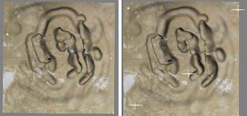
For this work, the environments have two types: static and dynamic. In static environment, as shown in Figure 7, there are no moving objects except for the agent, unlike the dynamic environment, in which there are three planes flying at the same altitude of the UAV, $p_{approAlt}$, and having a constant speed. The initial positions of the goal point and the agent are randomly defined at the beginning of every episode. The episode will be done if one of the three criteria is met: First, the agent reaches the goal; second, the agent collides; third, the agent runs out of steps. For our AUN framework, 5,000 episodes of training approximately took 36 hours for moderate computers.

Figure 7. Left: static environment (no moving objects except the agent). Right: dynamic environment (there are three moving planes).

Trajectories Classification

After iteratively calculating the SSE, 4,000 was optimal $k$ picked up by the elbow method for range 100–6,000 with 100 interval size. The 200,000 states randomly sampled from the 5,000 episodes training replay buffer were used to train the PSAE and to measure the performance between the PSAE and the convolution based one-shot learning. The standard deviation (SD) was used to indicate the spread of the data distributions from both methods.

Figure 8. Data distributions in clusters. Left: of one-shot learning. Right: of PSAE.

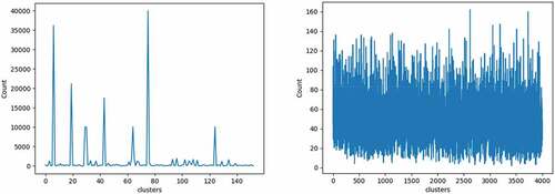
As shown in Figure 8, it was obvious that the data distribution of PSAE was of a much lower concentration than that of the one-shot learning and had an SD at 24.89. For one-shot learning, the data were largely concentrated on just four clusters and had an SD at 5,017.52. Despite this huge difference, it may not be sufficient to judge which one is better for AUN. So, the results in the AUN task were compared once more to confirm the performance of each method.

Figure 9. Success rates of using TD3 with ABR (one-shot learning) and ABR+ (PSAE). Left: in static environment. Right: in dynamic environment. (The figure is designed for coloured version.)

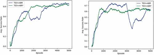
As shown in Figure 9, the success rates in AUN task of PSAE (ABR+) and one-shot learning (ABR) were so close. For static environments, the success rates were 82.4%, 84.8%, respectively, and 61.6%, 63.2% for dynamic environments. But what can be seen clearly is that the PSAE helps to make the learning process significantly more stable.

Autonomous UAV Navigation

If we consider the fact that FORK relies on learning the reward function to improve the policy, then the rewarding in ABR, in which reward fluctuates according to the rank of trajectory, may suffer the reward forecasting process. Therefore, we tested FORK on AUN with both TR and ABR+. The results on the static environment of the proposed method and TD3-FORK are shown in Figure 10.

Figure 10. Results of using TD3-FORK with TR, ABR+, and TD3-LG with ABR+ in static environment. Left: success rate. Right: collision rate (the out-of-step rate is a residual from success and collision rates). (The figure is designed for coloured version.)

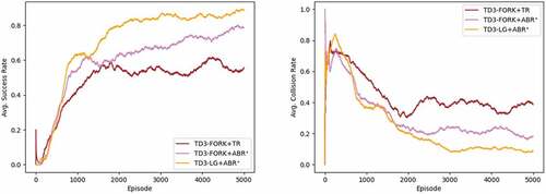
The TD3-LG+ABR+ (proposed) achieved the highest success rate, which is 88.6%, and for TD3-FORK, it is 55.8% and 78.6% for TR and ABR+, respectively. This result is again the evidence that the drawbacks of TR outweigh the benefits. In terms of collision rates, TD3-LG+ABR+ received 8.8% and 38.6% and 18.2% for TR and ABR+ of TD3-FORK, respectively.

Figure 11. Results of using TD3-FORK with ABR+ and TD3-LG with ABR+ in dynamic environment. Left: success rate. Right: collision rate. (The figure is designed for coloured version.)

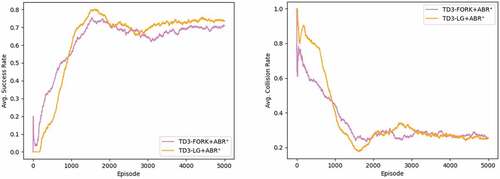
As shown in Figure 11, in dynamic environment, the success rate of TD3-LG+ABR+ dropped to 73.4%, which is 15% lower from the static. Conversely, TD3-FORK+ABR+ was somewhat able to maintain the same performance, which is 71% (7% lower). The collision rates were 25.6% and 25.2% for TD3-LG and TD3-FORK, respectively.

Complexity

We also measured the improvement in terms of complexity. Our two methods (LG, ABR+) mainly utilized the DNN; so, their computational complexity can be formulated as follows:

(16) $c_{LG}=O\left(N_h{M}^2\right)$(16)

where $c_{LG}$denotes the computational complexity of LG and $N_h,M$ denote number of hidden layers in DNN and maximum number of neurons in layer, respectively.

As can be seen in Equation 3.1, the computational complexity of ABR+ depends on the number of transitions in an episode. Hence, it can be done as follows:

(17) $c_{\mathrm{A}\mathrm{B}{\mathrm{R}}^{+}}=O\left(T\left(\left(N_{PSAE}{M_{PSAE}}^2\right)+\left(N_C{M_C}^2\right)\right)\right)$(17)

where $c_{\mathrm{A}\mathrm{B}{\mathrm{R}}^{+}}$ denotes the computational complexity of ABR+ and $N,M$denote the number of hidden layers and maximum number of neurons for DNNs of features extraction (PSAE) and trajectories classification. $T$ denotes the number of transitions in an episode.

But, in RL, only computational complexity is insufficient to tell how fast the method is. So, we decided to use the straighter way, the sample complexity. It is the number of training steps (million) required to reach the same point. In this work, the best success rates of TD3-FORK+ABR+ were used as the point, which are 78% and 74% for static and dynamic environments, respectively.

Table 2. Sample complexity (million steps) of TD3-FORK+ABR+ and TD3-LG+ABR+.

Environment	TD3-FORK+ABR+	TD3-LG+ABR+
Static environment	0.95	0.41
Dynamic environment	0.39	0.32

As shown in Table 2, in the static environment, TD3-FORK+ABR+ required 0.95 million training steps to achieve its best success rate (78%) and TD3-LG+ABR+ only needed 0.41 million steps to reach the same success rate, reducing the training steps by more than 50%. But, in the dynamic environment, the numbers were not much different; the required training steps for TD3-LG+ABR+ were 18% lower than those of TD3-FORK+ABR+.

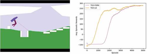
Other Navigation Task

To confirm the performance of the proposed method, we performed a test on the BipedalWalkerHardcore, which is the navigation task most similar to AUN for the well-known series of RL tasks, the OpenAI gym (Brockman et al. 2016). Wei and Ying (2020) suggested the three heuristic changes to overcome this tough task. Two of the three in the changes are modifying the reward so, to get along, the ABR+ was not put to this experiment. The result of TD3-FORK for this task was earned from running their source code, which was provided on online websites, on our computer. In terms of TD3-LG, we simply used the same as for AUN but under the three heuristic changes. The results are shown in Figure 12:

Figure 12. Left: BipedalWalkerhardcore task. Right: episodic rewards of using TD-FORK and TD-LG in BipedalWalkerhardcore task. (The figure is designed for coloured version).

Conclusion

This work proposed the LG and PSAE algorithms to achieve more successes from AUN task and to address the apprehensive behavior of the agent. The experimental results proved that the proposed method is more efficient than both the state-of-the-art method (TD3-FORK) and our previous method, TD3-ABR. In the AUN task, the proposed method achieved 88.6% and 73.4% success rates for the static and dynamic environments, respectively, which are 10% and 2.4%, respectively, greater than the state-of-the-art method in the static and dynamic environments. The higher success rates were caused by the absence of apprehensive behavior. If you notice the collision rates in the dynamic environment of all methods, it all were nearly equal to 25%, but for the proposed method, the amount of out-of-step episodes was significantly low (the out-of-step episodes are residual from the collision and success episodes). In general, if the collision punishment is low like in the proposed method, the agent will become reckless and never converge to a good result. But using the punishment through the policy update process of LG instead helps the agent stay in equilibrium between venturous and careful. In addition, even though the results of LG and FORK in BipedalWalkerHardcore are very close, the computational burden of LG is lower at least two times since it uses only one smaller network.

However, the proposed method has two drawbacks. First, the PSAE needs to be trained on training set having comprehensive patterns of trajectory before being used in ABR+. Second, like FORK, the hyper-parameter controlling the level of policy adjustment somewhat influences the performance.

Disclosure statement

No potential conflict of interest was reported by the authors.

References

- Apostolopoulos, P. A., M. Torres, and E. Eleni Tsiropoulou. 2019. Satisfaction-aware data offloading in surveillance systems. Proceedings of the 14th Workshop on Challenged Networks - CHANTS’19. doi:10.1145/3349625.3355437.
- Bellman, R. 1957. A Markovian decision process. Indiana University Mathematics Journal 6 (4):679–3286. doi:10.1512/iumj.1957.6.56038.
- Brockman, G., V. Cheung, L. Pettersson, J. Schneider, J. Schulman, J. Tang, and W. Zaremba. 2016. OpenAI gym. arXiv. doi:10.48550/ARXIV.1606.01540.
- Castaño, A. R., H. Romero, J. Capitán, J. Luis Andrade, and A. Ollero. 2019. Development of a semi-autonomous aerial vehicle for sewerage inspection. Advances in Intelligent Systems and Computing November (November):75–86. doi:10.1007/978-3-030-35990-4_7.
- Chansuparp, M., and K. Jitkajornwanich. 2022. A novel augmentative backward reward function with deep reinforcement learning for autonomous UAV navigation. Applied Artificial Intelligence 36 1 .
- Elmokadem, T., and A. V. Savkin. 2021. A hybrid approach for autonomous collision-free UAV navigation in 3D partially unknown dynamic environments. Drones 5 (3):57. doi:10.3390/drones5030057.
- Fujimoto, S., van Hoof, and D. Meger. 2018. Addressing function approximation error in actor-critic methods. ArXiv Org. https://arxiv.org/abs/1802.09477.
- Guo, T., N. Jiang, B. Li, X. Zhu, Y. Wang, and W. Du. 2020. UAV navigation in high dynamic environments: A deep reinforcement learning approach. Chinese Journal of Aeronautics 34 (2):479–89, June. doi:https://doi.org/10.1016/j.cja.2020.05.011.
- Haarnoja, T., Z. Aurick, H. Kristian, T. George, H. Sehoon, T. Jie, K. Vikash, Z. Henry, G. Abhishek, A. Pieter, et al. 2018. Soft actor-critic algorithms and applications. arXiv. doi:10.48550/ARXIV.1812.05905.
- Haarnoja, T., A. Zhou, P. Abbeel, and S. Levine. 2018. Soft actor-critic: Off-policy maximum entropy deep reinforcement learning with a stochastic actor. arXiv. doi:10.48550/ARXIV.1801.01290.
- Hawary, A. F., and N. A. Razak. 2018. Real-time collision avoidance and path optimizer for semi-autonomous UAVs. IOP Conference Series: Materials Science and Engineering 370 (May):012043. doi:10.1088/1757-899x/370/1/012043.
- Jain, T., A. Sibley, H. Stryhn, and I. Hubloue. 2018. Comparison of unmanned aerial vehicle technology-assisted triage versus standard practice in triaging casualties by paramedic students in a mass-casualty incident scenario. Prehospital and Disaster Medicine 33 (4):375–80. doi:10.1017/s1049023x18000559.
- Kapturowski, S., G. Ostrovski, J. Quan, R. Munos, and W. Dabney. 2018. Recurrent experience replay in distributed reinforcement learning. Openreview.net. Accessed September 27, 2018. https://openreview.net/forum?id=r1lyTjAqYX
- Koenig, N., and A. Howard. n.d.. 2004. Design and use paradigms for gazebo, an open-source multi-robot simulator. 2004 IEEE/RSJ International Conference on Intelligent Robots and Systems (IROS) (IEEE Cat. No.04CH37566). Accessed October 20, 2019. doi:10.1109/iros.2004.1389727.
- Lillicrap, T. P., J. J. Hunt, A. Pritzel, N. Heess, T. Erez, Y. Tassa, D. Silver, and D. Wierstra. 2015. Continuous control with deep reinforcement learning. ArXiv Org. https://arxiv.org/abs/1509.02971.
- Liu, F., and Y. Deng. 2021. Determine the number of unknown targets in open world based on elbow method. IEEE Transactions on Fuzzy Systems 29 (5):986–95. doi:10.1109/tfuzz.2020.2966182.
- Lu, Y., Z. Xue, G.-S. Xia, and L. Zhang. 2018. A survey on vision-based UAV navigation. Geo-Spatial Information Science 21 (1):21–32. doi:10.1080/10095020.2017.1420509.
- Maciel-Pearson, B. G., L. Marchegiani, S. Akcay, A. Atapour-Abarghouei, J. Garforth, and T. P. Breckon. 2019. Online deep reinforcement learning for autonomous UAV navigation and exploration of outdoor environments. ArXiv:1912 05684 [Cs] December (December). https://arxiv.org/abs/1912.05684.
- Meng, L., R. Gorbet, and D. Kulić. 2021. The effect of multi-step methods on overestimation in deep reinforcement learning. Στο 2020 25th International Conference on Pattern Recognition (ICPR), 347–53. doi:10.1109/ICPR48806.2021.9413027.
- Mittal, D., D. Gaurav, and S. Sekhar Roy. 2015. An effective hybridized classifier for breast cancer diagnosis. 2015 IEEE International Conference on Advanced Intelligent Mechatronics (AIM), July. doi:10.1109/aim.2015.7222674.
- Ng, A. 2011. Sparse autoencoder. CS294A Lecture Notes https://web.stanford.edu/class/cs294a/sparseAutoencoder_2011new.pdf.
- Qiu, X., Z. Yao, F. Tan, Z. Zhu, and L. Jun-Guo. 2020. One-to-one air-combat maneuver strategy based on improved TD3 algorithm. Στο 2020 Chinese Automation Congress (CAC) 5719–25. doi:10.1109/CAC51589.2020.9327310.
- Rummery, G. A., and M. Niranjan. 1994. On-line Q-learning using connectionist systems. Undefined. https://www.semanticscholar.org/paper/On-line-Q-learning-using-connectionist-systems-Rummery-Niranjan/7a09464f26e18a25a948baaa736270bfb84b5e12
- Sadeghzadeh-Nokhodberiz, N., A. Can, R. Stolkin, and A. Montazeri. 2021. Dynamics-based modified fast simultaneous localization and mapping for unmanned aerial vehicles with joint inertial sensor bias and drift estimation. IEEE Access 9:120247–60. doi:10.1109/access.2021.3106864.
- Schneider, S., G. W. Taylor, S. Linquist, and S. C. Kremer. 2019. Similarity learning networks for animal individual re-identification – Beyond the capabilities of a human observer. arXiv. doi:10.48550/ARXIV.1902.09324.
- Shi, C., B. Wei, S. Wei, W. Wang, H. Liu, and J. Liu. 2021. A quantitative discriminant method of elbow point for the optimal number of clusters in clustering algorithm. EURASIP Journal on Wireless Communications and Networking 2021 (1). doi:10.1186/s13638-021-01910-w.
- Stanford Artificial Intelligence Laboratory et al. 2018. Robotic operating system (version ROS melodic morenia). https://www.ros.org
- Sudhakar, S., V. Vijayakumar, C. Sathiya Kumar, V. Priya, L. Ravi, and V. Subramaniyaswamy. 2020. Unmanned Aerial Vehicle (UAV) based forest fire detection and monitoring for reducing false alarms in forest-fires. Computer Communications 149:1–16. doi:10.1016/j.comcom.2019.10.007.
- Vincent, P., H. Larochelle, Y. Bengio, and P.-A. Manzagol. 2008. Extracting and composing robust features with denoising autoencoders. Proceedings of the 25th International Conference on Machine Learning - ICML ’08. doi:10.1145/1390156.1390294.
- Wei, H., and L. Ying. 2020. FORK: A forward-looking actor for model-free reinforcement learning. arXiv. doi:10.48550/ARXIV.2010.01652.
- Youn, W., H. Ko, H. Choi, I. Choi, J.-H. Baek, and H. Myung. 2020. Collision-free autonomous navigation of a small UAV using low-cost sensors in GPS-denied environments. International Journal of Control, Automation, and Systems 19 (2):953–68. doi:10.1007/s12555-019-0797-7.
- Zhang, L., S. Han, Z. Zhang, L. Li, and S. Lü. 2020. Deep recurrent deterministic policy gradient for physical control. Artificial Neural Networks and Machine Learning – ICANN 2020:257–68. doi:10.1007/978-3-030-61616-8_21.
- Zhang, F., J. Li, and Z. Li. 2020. A TD3-based multi-agent deep reinforcement learning method in mixed cooperation-competition environment. Neurocomputing 411 (October):206–15. doi:10.1016/j.neucom.2020.05.097.
- Zhang, Z., L. XinHong, A. JiPing, W. Man, G. Zhang, and M. Pizzarelli. 2020. Model-free attitude control of spacecraft based on PID-guide TD3 algorithm. Edited by Marco Pizzarelli. International Journal of Aerospace Engineering. 2020 (December):1–13. doi:10.1155/2020/8874619.
- Zhang, Q., M. Zhu, L. Zou, M. Li, and Y. Zhang. 2020. Learning reward function with matching network for mapless navigation. Sensors 20 (13):3664. doi:10.3390/s20133664.
- Zijian, H., K. Wan, X. Gao, Y. Zhai, and Q. Wang. 2020. Deep reinforcement learning approach with multiple experience pools for UAV’s autonomous motion planning in complex unknown environments. Sensors 20 (7):1890. doi:10.3390/s20071890.
- Zonneveld, T. V. 2018. Realisation of a safety-cage with integrated force sensing for interactive aerial robots. Essay.utwente.nl. Accessed July 6, 2018. https://essay.utwente.nl/75255/