Yield-SpikeSegNet: An Extension of SpikeSegNet Deep-Learning Approach for the Yield Estimation in the Wheat Using Visual Images

ABSTRACT

High-throughput plant phenotyping integrated with computer vision is an emerging topic in the domain of nondestructive and noninvasive plant breeding. Analysis of the emerging grain spikes and the grain weight or yield estimation in the wheat plant for a huge number of genotypes in a nondestructive way has achieved significant research attention. In this study, we developed a deep learning approach, “Yield-SpikeSegNet,” for the yield estimation in the wheat plant using visual images. Our approach consists of two consecutive modules: “Spike detection module” and “Yield estimation module.” The spike detection module is implemented using a deep encoder-decoder network for spike segmentation and output of this module is spike area and spike count. In yield estimation module, we develop machine learning models using artificial neural network and support vector regression for the yield estimation in the wheat plant. The model’s precision, accuracy, and robustness are found satisfactory in spike segmentation as 0.9982, 0.9987, and 0.9992, respectively. The spike segmentation and yield estimation performance reflect that the Yield-SpikeSegNet approach is a significant step forward in the domain of high-throughput and nondestructive wheat phenotyping.

Introduction

Wheat is considered one of the most crucial crops from the universal perspective. It contributes a significant percentile of the protein and calories needed in the human diet (Tilman et al. 2011). Rapid population growth and speedy urbanization in developing countries are the major factors behind the extreme hike in food demand. Additionally, the effect of seasonal fluctuation and climate changes that lead to inconsistent wheat supply need to be addressed. Therefore, identifying the high-yielding and stress (biotic and abiotic) tolerance wheat genotypes is the key challenge to wheat breeders. Genotyping and phenotyping are the two main pillars in the genetic improvement of the crop. Though genotyping is done with greater accuracy, traditional phenotyping involves too many challenges. The genotype-phenotype gap is one of the most problematic zones in the domain of modern plant breeding (Großkinsky et al. 2015; Houle, Govindaraju, and Omholt 2010). Plant phenomics research has been gaining momentum recently to address this bottleneck. As traditional phenotyping is destructive, tedious and time-consuming, nondestructive and high-throughput plant phenotyping is needed in this context (Campbell et al. 2017). High-dimensional imaging sensors based plant phenotyping platforms were developed by several researchers (Fahlgren et al. 2015; Großkinsky et al. 2015; Hartmann et al. 2011; Houle, Govindaraju, and Omholt 2010; Rahaman et al. 2015) to cope up with the challenges. Analysis of the emerging grain spikes is one of the important phonological events in wheat development phases to study the application of agricultural inputs (water, fertilizer, etc.). Besides, yield or grain weight estimation has gained significant research attention. But, the manual process of yield estimation is destructive, tedious, and time-consuming as it involves separating spikelets from the spikes and taking weight using a weighing machine. Therefore, nondestructive and automated spike detection and correspondingly yield estimation models are essential as a fast alternative.

Recently, image analyses, specifically computer-vision based approaches, are gaining momentum (Alharbi, Zhou, and Wang 2018; Bi et al. 2010; Grillo, Blangiforti, and Venora 2017; Hasan et al. 2010; Misra et al. 2020, 2021a, 2021b; Pound et al. 2017; Qiongyan et al. 2017; Tan et al. 2020; Tanuj et al. 2019). Further, it is strongly proposed by Tsaftaris, Minervini, and Scharr (2016) that the future trends of plant phenotyping will depend on the combined effort of image analysis and machine learning. Grillo, Blangiforti, and Venora (2017) developed a new method based on computer-aided glume image analysis for identifying wheat local landraces. They applied linear discriminate techniques by utilizing quantitative morpho-colorimetric variables. The overall percentage of correct identification was 89.7%. Alharbi, Zhou, and Wang (2018) built a screening system to estimate the number of wheat spikes from wheat plant images. The system involved a transformation of the raw image using the color index of vegetation extraction followed by segmentation to reduce the background noises. Gabor filter banks and K-means clustering algorithm were used in the wheat ears detection, and the number of wheat spikes was estimated through the regression method. Tan et al. (2020) applied a simple linear iterative clustering technique on the digital image of wheat plants for super-pixel segmentation. After that, they applied support vector machine and k-nearest neighborhood methods on the super-pixels for the spike recognition. Bi et al. (2010) proposed spike traits (awn number, average awn length, and spike length) extraction methods based on morphology. They designed three-layer back-propagation neural networks for wheat species classification. Hasan et al. (2010) proposed spike detection and counting technique from wheat field images using a region-based convolutional neural network (R-CNN) with a high robustness score. Pound et al. (2017) contributed an annotated crop image dataset of wheat and implemented a multi-task deep neural network for localizing wheat spikes and spikelets. Qiongyan et al. (2017) developed a novel technique involving color indexing method for the plant segmentation and neural networks with Laws texture energy for spike identification. Our previous work (Misra et al. 2020, 2021a) developed a segmentation network, “SpikeSegNet,” for spike detection and counting from visual images of the wheat plant. The network consisted of two cascaded feature networks for local patch extraction and global mask refinement. We achieved high accuracy and robustness in spike detection and counting, irrespective of different illumination factors. In this article, we proposed the Yield-SpikeSegNet approach for yield estimation in visual images of wheat plants. Yield-SpikeSegNet is an extension of the SpikeSegNet approach. The proposed approach deals with the output of SpikeSegNet, which is fed as input to the machine learning model to estimate the plant’s yield or grain weight. In this study, we implemented the algorithm of SpikeSegNet, conducted a validation study to examine the segmentation performance of the network in spike detection, and developed a machine learning model to estimate the yield of the wheat plant from the visual images.

The article is divided into four sections. Section 1 (Introduction) enlighten the importance of wheat crop, global challenges faces in crop production, the role of high-throughput and nondestructive plant phenotyping, and the importance of computer vision approaches in wheat spike phenotyping. Section 2 (Materials and Methods) explains the image acquisition and imaging facility used, ground-truth preparation for the model development, deep learning architecture of the spike detection and yield estimation network, training mechanism, and performance metrics to evaluate the performance of the Yield-SpikeSegNet model. Section 3 (Result and Discussion) presents and discusses the model’s performance in spike detection and yield estimation. Finally, section 4 (Conclusion) highlights the summarization of the work, its extended applicable areas, and future scope.

Materials and Methods

Image Acquisition

We planted the wheat experiment in pots in Nanaji Deshmukh Plant Phenomics Centre, ICAR-Indian Agricultural Research Institute, New Delhi, India (28.6377° N, 77.1571° E). LemnaTec facilities (LemnaTecGmbH, Aachen, Germany) are installed in the phenomics center. The greenhouse climate was maintained with the temperature 250C, relative humidity 55% by keeping in mind the objective of providing optimum conditions for the growth. The recombinant inbred lines (RIL) population developed from parents, namely C306 x HD2967(185 RILs) including parents, were grown in plastic pots filled with 12.5 kg soil with a recommended dose of fertilizer (120-80-60 kg/ha N-P-K respectively) for this experiment for screening the best RILs under drought conditions. Plants were grown under controlled environmental conditions, and soil moisture-based irrigation was done. For the control plant, we kept the soil moisture 18% level. Then, drought was imposed by holding the water and allowing the soil moisture to drop down at 10%, and after that, irrigation was done up to 18% level. Such practices were followed after reproductive phase till the end of the experiment. Visual images (400 to 700 nm) of the wheat plants grown in the pots were captured using PROSILICA GT6600 (LemnaTecGmbH, Aachen, Germany) camera with a sensor resolution of 6576 × 4384 pixels. We took images in the reproductive stages of the plant as the spikes emerged in the same stage and maintained a constant white background in the imaging chamber to increase background separation accuracy from the plant parts in the image pre-processing tasks. Three direction images (0°, 120°, 240°) with respect to the plant initial position (0°) were recorded with the help of lifting and rotating unit residing in the imaging chamber. The different directions were considered to capture the overlapping parts of the plant.

Ground-Truth Preparation

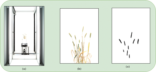
After imaging, we recorded the number of spikes and yield or grain weight corresponding to each plant manually to build the machine learning model for the yield estimation. As the sensor size is 6576 × 4384 pixels, it covers not only the plant parts but also the other parts of the chamber (Figure 1a). Therefore, we cropped (1656 × 1356 pixels) the images to get the region of interest (plant parts), as shown in Figure 1b. For developing the segmentation network, we prepared the ground truth segmented mask images corresponding to the cropped images manually, using the “wand tool” of Photoshop software. In the ground truth segmented mask image, black pixels represent the spikes shown in Figure 1c. For the ground-truth preparation, we followed the procedure mentioned in the “Dataset preparation” section of Misra et al. (2020).

Figure 1. (a) Plant image taken using LemnaTec facility covers not only the plant parts but also the other parts of the chamber, (b) cropped image to get the region of interest (plant parts), (c) ground truth segmented mask images corresponding to the cropped image.

Architecture of Yield-SpikeSegNet

Architecture of the Yield-SpikeSegNet is an extension of the SpikeSegNet approach (Misra et al. 2020, 2021) inspired by UNet (Ronneberger, Fischer, and Brox 2015) which is popularly used in pixel-wise segmentation of the object. Architecture of the Yield-SpikeSegNet consists of two modules namely, Spike detection module and Yield estimation module as shown in Figure 2. The Spike detection module is responsible for the detection or segmentation of spikes while Yield estimation module deals with the development of machine learning model by using the output of the previous module for the yield estimation corresponding to each plant.

Figure 2. Architecture of Yield-SpikeSegNet consisting of spike detection and yield estimation module.

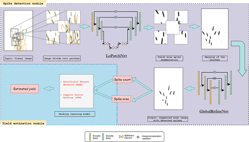
Spike Detection Module

The input of this module is the visual image (size: 1656 × 1356) of the wheat plant. The input image is divided into patches of size 256 × 256 to learn the local or critical features more efficiently than the bigger size image (Jha et al. 2020). The module consists of two essential feature networks in successive order: Local Patch Extraction Network (LoPatchExNet) and Global Purifying Network (GlobalPurifyNet). LoPatchExNet is used for extracting and learning the contextual and critical or local features more effectively in the patch level, and the GlobalPurifyNet helps in purifying or refining the output of LoPatchExNet, i.e., the segmented mask image, that possibly consists of some imprecise segmentation of object. The details of the feature network are highlighted in Misra et al. (2020, 2021). Convolutional encoder-decoder and stacked hourglass worked as the backbone of the LoPatchExNet and GlobalPurifyNet. The encoder is used to generate the feature map holding the contextual and spatial information from the input visual image, and the decoder uses the information as input to produce the corresponding segmented mask as output. Stacked hourglass is used to compress the incoming feature representation to facilitate more effective segmentation by focusing on the most important features irrespective of different viewpoints, scales, and illusions (Ronneberger, Fischer, and Brox 2015). The design and architecture of encoder-decoder and stacked hourglass are inspired by Misra et al. (2020, 2021) and Ronneberger, Fischer, and Brox (2015) and their numbers for constructing the LoPatchExNet and GlobalPurifyNet are estimated empirically for obtaining the optimum segmentation performances.

LoPatchExNet

The architecture of the LoPatchExNet comprises of encoding network [19], decoding network (Mao, Shen, and Yang 2016), and bottleneck network (with stacked hourglasses (Ronneberger, Fischer, and Brox 2015) in between the encoding and decoding network. The encoding network comprises hree encoder blocks consecutively, where output feature maps of one encoder block will work as input of another encoder block. Every encoder block comprises consecutive sets of dual 3 × 3 convolution operations with stride 1 and padding 1. Stride 1 refers that the filter of size 3 × 3 will move 1 pixel at a time. Padding 1 implies that one-pixel border will add to the input image with pixel value 0 for capturing the maximum information from the corner side of the image. Convolution operations succeeded by rectified linear activation unit (ReLU) (Agostinelli et al. 2014) and batch normalization (Ioffe and Szegedy 2015). Batch normalization is done by re-centering and re-scaling the input to make the network faster and stable. The whole set is succeeded by a max-pool operation with window size 2 × 2 and stride 2 by which the features are down-sampled and the aggregate features are extracted more efficiently. Pictorial representation of single encoder block is given in Figure 2. The structures of three encoder blocks in the encoding network are similar but only varying with different filter depths, i.e., 16, 64, 128 for the first, second, and third encoder blocks. The decoding network comprises three decoder blocks consecutively, where output feature maps of one decoder block will work as input of another decoder block. Each decoder block contains dual 3 × 3 convolution operations followed by ReLU and batch normalization, which is quite similar to the structure of the encoder block. But, the max-pool operation is replaced by transpose convolution (Ronneberger, Fischer, and Brox 2015) to up-sample the features. The features are then merged to the corresponding encoded feature maps for better localization. The three decoder blocks of the decoder network have 128, 64, and 16 number of filter depths as opposite to the encoder network. Bottleneck network lies in between encoder and decoder network. It consists of hourglasses for more confident segmentation irrespective of various effects like occlusion, scale, and view-points. The hourglasses again consist of hourglass-encoder and hourglass-decoder that are realized as residual blocks (Jha et al. 2020). The residual block facilitates the flow of spatial and gradient information throughout the deep network, which helps to solve the vanishing gradient descent problem. The number of hourglasses was decided empirically, and details of the inner structure of the hourglasses are discussed in our previous research work (Misra et al. 2020, 2021).

GlobalPurifyNet

The output of LoPatchExNet is a segmented mask image as given in Figure 2. However, it contains some inaccurate segmentation of spikes which misleads the determination of spike area and spike count. GlobalPurifyNet is responsible for refining the output of LoPatchExNet. The architecture of GlobalPurifyNet is similar to LoPatchExNet without the bottleneck network. The hyper-parameter, input-output and the inner structure of each encoder and decoder are discussed in the previous section.

Yield Estimation Module

This module deals with the output of Spike detection module i.e., segmented mask image with detected spikes. Segmented mask image is a binary image consisting of 0 (=black) and 1 (=white) pixel values. Here, black pixels denote the spike pixels and white pixels as non-spike pixels. Object count and area measurement is a common practice in binary image analysis domain. In this study, object is nothing but the spike. Flood-fill technique (Asundi and Wensen 1998) is applied on the segmented mask image for spike count and area measurement. The technique achieved object count and area measurement by rising through similar pixel regions from the start pixel until it discovers the edge of the object. Then outline it and continue the process for the whole image. Spike area and spike count are used as input for developing the machine learning model viz. artificial neural network (ANN) and support vector regression (SVR) for the yield estimation.

ANN

It is a statistical modeling approach based on biological neural systems’ structural and functional characteristics. ANN is made up of some interlinked processing elements called neurons or nodes. The input signal received by each neuron is the aggregate “information” coming from other neurons, which is processed through activation function and transferred to the other neurons or external neurons. The ANN is one of the suitable approaches for mapping the nonlinear relationship between input and output variables Equation (1)(1) $y_{i=}f\left(x_{i1,}{x}_{i2,}{x}_{i3,}\dots ,x_{ip,}w\right)+{ϵ}_i$(1) .

(1) $y_{i=}f\left(x_{i1,}{x}_{i2,}{x}_{i3,}\dots ,x_{ip,}w\right)+{ϵ}_i$(1)

where $x_{i1},x_{i2},x_{i3},\dots ,x_{ip}$ are the input variable; $y_i$ is the output variable; $w$ is the weight; ${ϵ}_i$ is the error term. An ANN, in general, comprises of three layers namely, input layers, hidden layers, and output layers. Input layers are in charge of receiving information (data), signals, features, or measurements from the external environments. In most cases, these inputs (samples or patterns) are normalized within the limit values produced by activation functions. Hidden layers are made up of neurons, which are in responsible of extracting patterns related to the processor system under investigation. Sigmoid activation function is frequently used in the hidden layer. Output layers, like input layers, are made up of neurons and are in responsible of producing and displaying the network’s final outputs. Gradient back propagation learning algorithm is used to determine ANN connection weights (Ray et al. 2020). The sum of a weighted combination of each neuron in the hidden layer is calculated using a nonlinear activation function f(s) and the formula below Equation (10)(10) $\mathrm{M}\mathrm{A}\mathrm{E}=\frac{1}{\mathrm{n}}{\sum }_{\mathrm{i}=1}^{\mathrm{n}}\left|{\mathrm{y}}_{\mathrm{i}}^{\mathrm{g}\mathrm{t}}-{\mathrm{y}}_{\mathrm{i}}^{\mathrm{p}\mathrm{r}\mathrm{e}\mathrm{d}}\right|$(10) .

(2) $s={\sum }_{i=1}^n{w}_i{x}_i+w_0$(2)

where, x_i is the input signal and $w_0$ is the bias term. Hyperbolic tangent function is the most commonly used activation function, and the bias term ($w_0$) is a constant added to the weight.

SVR

It is based on the idea of locating the best hyper-plane for dividing a dataset into two classes. It is based on Boser, Guyon, and Vapnik’s statistical learning theory (1992) (Isabelle, Guyon, and Vapnik 1992). Consider the vector of data set $Z=x_{\left(i\right)}{y}_{i\left(i=1\right)}N$, where $x_i\epsilon R^n$ contains both the vector of input and the scalar output, and N is the number of data points. The nonlinear SVR equation is as follows Equation 10(10) $\mathrm{M}\mathrm{A}\mathrm{E}=\frac{1}{\mathrm{n}}{\sum }_{\mathrm{i}=1}^{\mathrm{n}}\left|{\mathrm{y}}_{\mathrm{i}}^{\mathrm{g}\mathrm{t}}-{\mathrm{y}}_{\mathrm{i}}^{\mathrm{p}\mathrm{r}\mathrm{e}\mathrm{d}}\right|$(10) :

(3) $f\left(x\right)=W^T\varphi \left(x\right)+b$(3)

Where $\mathrm{\Phi }\left(\mathrm{x}\right):R_n\to R^{nh}$

is a nonlinear mapping function from the input space to a higher dimensional feature space with infinite dimension; $W\epsilon R^{nh}$ is weight vector; b is bias and T is transpose.

Performance of the SVR modeling is heavily reliant on the choice of Kernel function and optimal sets of hyper-parameters. The commonly used kernel functions are radial basis, polynomial, sigmoidal, and linear (Vapnik 1998).

Training of the Network

Training of the Spike Detection Module

Spike detection model consisting of LoPatchExNet and GlobalPurifyNet was trained by considering 900 images of 300 plants of 3-directions. The image dataset was randomly divided into training and testing at 80% and 20% ratios. First, LoPatchExNet and then GlobalPurifyNet were trained sequentially and later combined to form the single spike detection model. We used Linux operating system with 64 GB RAM and NVIDI GeForce GTX 1080 Ti Graphics (10 GB) to build the network model. We trained the network for 250 epochs and recorded the training losses at each epoch. Batch size was 32 images of size 256 × 256 as per the system constraints. The popular optimizer “Adam” (Kingma and Ba 2014) with a learning rate of 0.0005 was used to update the weight of the hidden nodes. Loss function was “Binary cross-entropy” (Dunne and Campbell 1997) as there are two classes (i.e., spikes and non-spikes) in this study.

Training of the Yield Estimation Module

The input of the yield estimation module is the output of the spike detection module (i.e., spike area and spike count). For developing the machine learning model (i.e., ANN SVM), the image dataset was divided into two parts randomly: 80% for training and 20% for testing. We fitted the Feed-Forward Multilayer Perceptron Neural Network by using the spike area and spike count as the input and the corresponding ground truth yield or grain weight as the output for the model’s training. The ANN architecture comprises one input layer with two input nodes (spike area and spike count) and one output layer with one node (ground truth yield). Although there is no firm hypothesis for determining the number of hidden layers and hidden nodes, distinctive combinations are attempted, and the best fitted ANN model is selected. We used the “Neuralnet” package of R software (Fritsch, Guenther, and Guenther 2019) for the model development. The same data points were used in training and testing the SVR model, and we built the model using the “e1071” (Meyer et al. 2019) package of R software.

Performance Metric

Performance Parameter for the Spike Detection Network

We measured the segmentation performance of the network model in spike detection using the statistical parameters viz. Mean segmentation error (Err I), Type {II error (Err II), Intersection over Union (IoU), Precision, Recall, and F-measure (Equations (4)(4) $PixClassEr{r}_t\left(O^{pred},O^{gt}\right)=\frac{1}{a\ast b}{\sum }_{j=1}^b{\sum }_{i=1}^a{O}^{pred}\left(i,j\right)\oplus O^{gt}\left(i,j\right)$(4) –(8(8) $\mathrm{I}\mathrm{o}\mathrm{U}=\frac{1}{\mathrm{C}}{\sum }_{\mathrm{i}=1}^{\mathrm{C}}\frac{{\mathrm{C}}_{\mathrm{i}\mathrm{i}}}{{\mathrm{G}}_{\mathrm{i}}+{\mathrm{P}}_{\mathrm{i}}-{\mathrm{C}}_{\mathrm{i}\mathrm{i}}}$(8) )). The pixel-wise segmentation performance was calculated on the resulting predicted segmented image (O^pred) of the spike detection module and the ground truth segmented image (O^gt). The details of the performance parameters are discussed below:

Mean Segmentation Error (Err I)

For calculating Err I, pixel-wise classification error (PixClassErr_t) of any test image t has been calculated as exclusive-OR operation between O^pred and O^gt of size a*b.

(4) $PixClassEr{r}_t\left(O^{pred},O^{gt}\right)=\frac{1}{a\ast b}{\sum }_{j=1}^b{\sum }_{i=1}^a{O}^{pred}\left(i,j\right)\oplus O^{gt}\left(i,j\right)$(4)

For every test image, (PixClassErr_t) has been calculated and finally the Err I is calculated by taking averages of (PixClassErr_t) of all the test images.

(5) $\mathrm{E}\mathrm{r}\mathrm{r}\mathrm{I}=\frac{1}{N}{\sum }_{t=1}^{N}PixClassEr{r}_t$(5)

Where, N = total number of test images. Err I is the probability value [0,1] where, large value (i.e., close to 1) represents the large error and small value (i.e., close to 0) implies the minimum error.

Type-II Error (Err II)

The main aim of Err II is to compute the disproportion among the apriori probabilities of spike and non-spike pixels for the overall test images. Err II of any tth test image (${\mathrm{E}\mathrm{r}\mathrm{r}}_{\mathrm{t}}^2$) is computed by doing average of the false positive rate (FPR) and false negative rate (FNR) at pixel level.

(6) $Er{r}_2^t=0.5\ast \mathrm{F}\mathrm{P}\mathrm{R}+0.5\ast \mathrm{F}\mathrm{N}\mathrm{R}$(6)

$\mathrm{F}\mathrm{P}\mathrm{R}=\frac{1}{a\ast b}{\sum }_{j=1}^b{\sum }_{i=1}^a\left(O^{gt}\left(i,j\right).\ast O^{pred}\left(i,j\right)\right)\oplus O^{pred}\left(i,j\right)$

$\mathrm{F}\mathrm{N}\mathrm{R}=\frac{1}{a\ast b}{\sum }_{j=1}^b{\sum }_{i=1}^a\left(O^{gt}\left(i,j\right).\ast O^{pred}\left(i,j\right)\right)\oplus O^{gt}\left(i,j\right)$

As similar to Err I, Err II is calculated by averaging the ${\mathrm{E}\mathrm{r}\mathrm{r}}_2^{\mathrm{t}}$ for all the test images as follows:

(7) $\mathrm{E}\mathrm{r}\mathrm{r}\mathrm{I}\mathrm{I}=\frac{1}{\mathrm{N}}{\sum }_{\mathrm{t}=1}^{\mathrm{N}}{\mathrm{E}\mathrm{r}\mathrm{r}}_2^{\mathrm{t}}$(7)

Where, N = total number of test images. Intersection over Union (IoU): IoU has been calculated using the following formula:

(8) $\mathrm{I}\mathrm{o}\mathrm{U}=\frac{1}{\mathrm{C}}{\sum }_{\mathrm{i}=1}^{\mathrm{C}}\frac{{\mathrm{C}}_{\mathrm{i}\mathrm{i}}}{{\mathrm{G}}_{\mathrm{i}}+{\mathrm{P}}_{\mathrm{i}}-{\mathrm{C}}_{\mathrm{i}\mathrm{i}}}$(8)

Where, C ( = 2) denotes the number of classes (i.e., spike and non-spike pixels); Cjj = number of pixels in any given image having the ground truth label j and the corresponding prediction is also j; Gj = number of pixels having ground truth class j; Pj = number of pixels having predicted class j.

The final IoU is calculated by taking average of all the test images. We have also calculated the precision, Recall, F-measures using True Positive (TP), True Negative (TN), False Positive (FP), and False Negative (FN). TP defines the number of pixels are rightly classified as spike pixels whereas TN denotes the number of pixels are rightly classified as non-spike pixels. FP implies the number of non-spike pixels classified as spike pixels and FN denotes the numbers of spike pixels are classified as non-spike pixels.

Performance Parameter for the Yield Estimation Network

Root Mean Square Error (RMSE): It is a good tool for the measurement of the performance of the prediction model. This tool is widely used for comparisons of several models’ performance and testing the efficiency. It is defined as the square root of the arithmetic mean of the squares of difference values between ground truth and predicted values. In this study, RMSE is computed as a measurement of the dispersion of the differences between the ground-truth grain weight or yield value (${\mathrm{y}}^{\mathrm{g}\mathrm{t}}$) and the predicted yield (${\mathrm{y}}^{\mathrm{p}\mathrm{r}\mathrm{e}\mathrm{d}}$) value .

(9) $\mathrm{R}\mathrm{M}\mathrm{S}\mathrm{E}=\sqrt{\frac{1}{\mathrm{n}}{\sum }_{\mathrm{i}=1}^{\mathrm{n}}{\left({\mathrm{y}}_{\mathrm{i}}^{\mathrm{g}\mathrm{t}}-{\mathrm{y}}_{\mathrm{i}}^{\mathrm{p}\mathrm{r}\mathrm{e}\mathrm{d}}\right)}^2}$(9)

Where, n is the number of observation. Mean Absolute Error (MAE): It is another model performance parameter that gives a linear score that means all the differences are equally weighted in the arithmetic mean. MAE is the arithmetic mean of the absolute values of the differences between ${\mathrm{y}}^{\mathrm{g}\mathrm{t}}$ and ${\mathrm{y}}^{\mathrm{p}\mathrm{r}\mathrm{e}\mathrm{d}}$

(10) $\mathrm{M}\mathrm{A}\mathrm{E}=\frac{1}{\mathrm{n}}{\sum }_{\mathrm{i}=1}^{\mathrm{n}}\left|{\mathrm{y}}_{\mathrm{i}}^{\mathrm{g}\mathrm{t}}-{\mathrm{y}}_{\mathrm{i}}^{\mathrm{p}\mathrm{r}\mathrm{e}\mathrm{d}}\right|$(10)

For the model’s comparison, the RMSE and MAE can be used together. The greater difference between RMSE and MAE indicates the greater the variance in the individual errors in the sample.

Results and Discussion

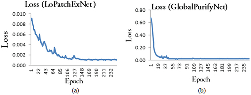
The Spike detection model was trained using randomly selected 720 images (i.e., 80% of the total image dataset) and validated with 180 images (i.e., 20% of the total image dataset). We trained LoPatchExNet and GlobalPurifyNet separately and later they were combined to form the spike detection model. As LoPatchExNet was trained at patch level and the size of the input image of LoPatchExNet is 256 × 256 pixels, the original images (of size 1656 × 1356 pixels) were divided into patches of size 256 × 256 pixels. The network was trained for 250 epochs and the training losses were initially high. It plateaued around 150 epochs (Figure 3a). The output of LoPatchExNet is segmented mask image of size 256 × 256 pixels at patch level. The patches were merged to construct the original image of size 1656 × 1356 pixels (Figure 2) which contains some inaccurate segmentation of spikes. These noises were refined at GlobalPurifyNet. The GlobalPurifyNet was developed using the same training and testing dataset as of LoPatchExNet. Although the model was trained for 250 epochs, a remarkable decrease of the losses was noticed and it plateaued around 48 epochs as shown in Figure 3b.

Figure 3. Training losses of (a) LoPatchExNet, and (b) GlobalPurifyNet.

Segmentation Performance of the Spike Detection Model

Segmentation performance of the spike detection model is evaluated on the test dataset (120 image data) using the above mentioned performance parameters (Err I, Err II, IoU, Precision, Recall, and F-measure). The average value of these parameters for the test dataset is given in Table 1.

Table 1. Segmentation performance.

Mean Segmentation error (Err I)	Type II error(Err II)	Intersection over Union (IoU)	Accuracy	Precision	Recall	F1Score
0:0017	0.0562	0.0562	0.9987	0.9982	0.9979	0.9992

Precision=TP/(TP+FP); Recall=TP/(TP+FN); Accuracy=(TP+TN)/(TP+TN+FP+FN); TP: True Positive; TN: True Negative; FP: False Positive; FN: False Negative.

As the segmentation performance is calculated at pixel level, the value of mean segmentation error (i.e., 0.0017) depicts that on an average only 111 pixels are classified wrongly. Precision value from Table 1 represents that on an average 99.82% of the detected pixels using the spike detection model are actually spike pixels. It is reflected from the recall value that, 99.79% of the actual spike pixels are identified among the ground-truth spike pixels. Accuracy and robustness of the model in spike segmentation are on an average 99.87% and 99.92%, respectively.

Performance Evaluation of the Yield Estimation Model

The independent variables for developing the ANN model are spike area and spike count whereas the dependent variable is the grain weight or yield. The model was trained using randomly selected 720 data points (i.e., 80% of the total image dataset) and tested using 180 data points (i.e., 20% of the total image dataset). Different combinations of hidden layers and hidden nodes were attempted on trial-and-error basis. Among them, one hidden layer with two hidden nodes out performed. The best fitted ANN model architecture is given in Figure 4. The performance parameters RMSE and MAE of the training and testing dataset are presented in Table 2.

Figure 4. Fitted ANN model architecture.

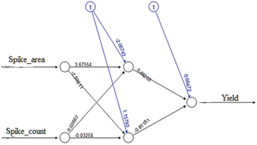
Table 2. Performance of ANN and SVR in training and testing dataset.

	ANN		SVR
Performance parameter	Training	Testing	Training	Testing
MAE	4.048552	3.851167	3.87128	3.87211
REMS	5.382943	5.223983	5.227	5.202683

Same data points were used in training and testing the SVR model. The optimal values of the hyper-parameters (i.e., cost, kernel width and insensitivity) on the basis of performance are given in Table 3. RMSE and MAE of the training and testing dataset are given in Table 2. Support vector was found as 609.

Table 3. Summary statistics of the hyper-parameters used in SVR model development.

Cost	Kernel width	Insensitivity	SVR-Kernel	SVR-type	Number of Support ector
1	0.5	0.1	Radial	Eps-regression	609

It can be depicted from Table 2 that in training dataset MAE of SVR is lower than of ANN. But, the difference is very low. In testing dataset, the performance of MAE in ANN and SVR are at per. In ANN, the difference of RMSE values between training and testing dataset is higher than of SVR. Hence, the generalization capability of SVR in this dataset is more than ANN. As a result, it can be concluded that SVR model is more appropriate than ANN in the dataset.

Conclusion

In the era of modern phenotyping, grain weight or yield estimation in the wheat plant for a huge number of genotypes in a nondestructive way is a challenging task. In this study, we proposed a deep learning approach, “Yield-SpikeSegNet,” for the yield estimation in the wheat plant using visual images. The model’s precision, accuracy, and robustness are satisfactory in spike segmentation as 99.82%, 99.87%, and 99.92%, respectively. It is depicted from the RMSE value that the generalization capability of SVR is more than ANN in the case of the yield estimation model. The architecture of “Yield-SpikeSegNet” has been developed with advanced technology integrated with deep encoder, decoder, and hourglasses. Because of this, it is a significant step forward in the domain of nondestructive and high-throughput wheat yield phenotyping.

Availability of Data and Materials

The datasets used and/or analyzed during the current study are available from the corresponding author on reasonable request.

Consent for Publication

Consent and approval for publication from all the authors was obtained.

Ethics Approval and Consent to Participate

Not applicable.

Acknowledgments

The first author acknowledges the fellowship received from ICAR-IASRI, New Delhi, India, to undertake this research work as part of his Ph.D. program and Nanaji Deshmukh Plant Phenomics Facility, ICAR-IARI, New Delhi, for the facilities. This work was supported by National Agriculture Science Fund (NASF), ICAR, Grant No.NASF/Phen-6005/2016-17 and NAHEP CAAST (NAHEP/CAAST/2018/19/07).”

Disclosure statement

No potential conflict of interest was reported by the author(s).

Additional information

Funding

This work was supported by National Agriculture Science Fund (NASF), ICAR, [Grant No.NASF/Phen-6005/2016-17] and NAHEP CAAST [NAHEP/CAAST/2018/19/07].

References

- Agostinelli, F., M. Hoffman, P. Sadowski, and P. Baldi. 2014. Learning activation functions to improve deep neural networks. arXiv preprint arXiv:1412.6830, December 21.
- Alharbi, N., J. Zhou, and W. Wang. 2018. Automatic counting of wheat spikes from wheat growth images. ICPRAM, 346–3302.
- Asundi, A., and Z. Wensen. 1998. Fast phase-unwrapping algorithm based on a gray-scale mask and flood fill. Applied Optics 37 (23):5416–20, August 10. doi:10.1364/AO.37.005416.
- Bi, K., P. Jiang, L. Li, B. Shi, and C. Wang. 2010 Non-destructive measurement of wheat spike characteristics based on morphological image processing. Transactions of the Chinese Society of Agricultural Engineering 26(12):212–16, December 1.
- Campbell, M. T., H. Walia, A. Grondin, and A. Knecht. 2017. Genetic and computational approaches for studying plant development and abiotic stress responses using image-based phenotyping AGU Fall Meeting Abstracts 2017:B41J–06, December.
- Dunne, R. A., and N. A. Campbell. 1997. On the pairing of the softmax activation and cross-entropy penalty functions and the derivation of the softmax activation function. Proceedings of the 8th Australian Conference on the Neural Networks, vol. 181, 185. Melbourne: Citeseer, June 30.
- Fahlgren, N., M. Feldman, M. A. Gehan, M. S. Wilson, C. Shyu, D. W. Bryant, S. T. Hill, C. J. McEntee, S. N. Warnasooriya, I. Kumar, et al. 2015 A versatile phenotyping system and analytics platform reveals diverse temporal responses to water availability in setaria. Molecular Plant 8(10):1520–35, October 5. doi:10.1016/j.molp.2015.06.005.
- Fritsch, S., F. Guenther, and M. F. Guenther. 2019. Package ‘neuralnet’ Training of Neural Networks. The R Journal, February 7.
- Grillo, O., S. Blangiforti, and G. Venora. 2017. A wheat landraces identification through glumes image analysis Computers and Electronics in Agriculture 141:223–31, September 1. doi:10.1016/j.compag.2017.07.024.
- Großkinsky, D. K., J. Svensgaard, S. Christensen, and T. Roitsch. 2015. Plant phenomics and the need for physiological phenotyping across scales to narrow the genotype-to-phenotype knowledge gap. Journal of Experimental Botany 66(18):5429–40, September 1. doi:10.1093/jxb/erv345.
- Hartmann, A., T. Czauderna, R. Hoffmann, N. Stein, and F. Schreiber. 2011. Htpheno: An image analysis pipeline for high-throughput plant phenotyping. BMC Bioinformatics 12(1):1–9, December. doi:10.1186/1471-2105-12-148.
- Hasan, M. M., J. P. Chopin, H. Laga, and S. J. Miklavcic. 2010. Detection and analysis of wheat spikes using convolutional neural networks. Transactions of the Chinese Society of Agricultural Engineering 26(12):212–16, December 1.
- Houle, D., D. R. Govindaraju, and S. Omholt. 2010. Phenomics: The next challenge. Nature Reviews Genetics 11(12):855–66, December. doi:10.1038/nrg2897.
- Ioffe, S., and C. Szegedy. 2015. Batch normalization: Accelerating deep network training by reducing internal covariate shift. International Conference on Machine Learning, 448–56. PMLR, June 1.
- Isabelle, B. B., M. Guyon, and V. N. Vapnik. 1992. A training algorithm for optimal margin classifiers. COLT, 92.
- Jha, R. R., G. Jaswal, D. Gupta, S. Saini, and A. Nigam. 2020. PixIsegnet: Pixel[u+2010]level iris segmentation network using convolutional encoder–decoder with stacked hourglass bottleneck. IET Biometrics 9(1):11–24, January. doi:10.1049/iet-bmt.2019.0025.
- Kingma, D. P., and J. Ba. 2014. Adam: A method for stochastic optimization. December 22.
- Mao, X., C. Shen, and Y. B. Yang. 2016. Image restoration using very deep convolutional encoder-decoder networks with symmetric skip connections. Advances in Neural Information Processing Systems 29:2802–10.
- Meyer, D., E. Dimitriadou, K. Hornik, A. Weingessel, F. Leisch, C. C. Chang, C.C. Lin, and M. D. Meyer. 2019. Package ‘e1071’. The R Journal November 26.
- Misra, T., A. Arora, S. Marwaha, V. Chinnusamy, A. R. Rao, R. Jain, R. N. Sahoo, M. Ray, S. Kumar, D. Raju, et al. 2020. SpikeSegnet-a deep learning approach utilizing encoder-decoder network with hourglass for spike segmentation and counting in wheat plant from visual imaging. Plant Methods 16(1):1–20, December. doi:10.1186/s13007-020-00582-9.
- Misra, T., A. Arora, S. Marwaha, R. R. Jha, M. Ray, R. Jain, A. R. Rao, E. Varghese, S. Kumar, S. Kumar, et al. 2021a. Web-SpikeSegnet: Deep learning framework for recognition and counting of spikes from visual images of wheat plants. IEEE Access 9:76235–47, May 17. doi:10.1109/ACCESS.2021.3080836.
- Misra, T., S. Marwaha, A. Arora, M. Ray, S. Kumar, S. Kumar, and V. Chinnusamy. 2021b. Leaf area assessment using image processing and support vector regression in rice. The Indian Journal of Agricultural Sciences 91(3 388–392), March 1
- Pound, M. P., J. A. Atkinson, D. M. Wells, T. P. Pridmore, and A. P. French. 2017. Deep learning for multi-task plant phenotyping. Proceedings of the IEEE International Conference on Computer Vision Workshops Venice, Italy, 2055–63.
- Qiongyan, L., J. Cai, B. Berger, M. Okamoto, and S. J. Miklavcic. 2017. Detecting spikes of wheat plants using neural networks with laws texture energy. Plant Methods 13(1):1–3, December. doi:10.1186/s13007-017-0231-1.
- Rahaman, M., D. Chen, Z. Gillani, C. Klukas, and M. Chen. 2015. Advanced phenotyping and phenotype data analysis for the study of plant growth and development. Frontiers in Plant Science 6:619, August 10. doi:10.3389/fpls.2015.00619.
- Ray, M., K.N. Singh, V. Ramasubramanian, R. K. Paul, A. Mukherjee, and S. Rathod. 2020. Integration of wavelet transform with ann and wnn for time series forecasting: an application to indian monsoon rainfall. National Academy Science Letters 43(6):509–13, November. doi:10.1007/s40009-020-00887-2.
- Ronneberger, O., P. Fischer, and T. Brox. 2015. U-net: Convolutional networks for biomedical image segmentation. International Conference on Medical Image Computing and Computer-assisted Intervention, 234–41. Cham: Springer, October 5.
- Tanuj, M., A. Alka, M. Sudeep, R. Mrinmoy, R. Dhandapani, K. Sudhir, G. Swati, R. N. Sahoo, and C. Viswanathan. 2019. Leaf area assessment using image processing and support vector regression in rice. Indian Journal of Agricultural Sciences 89 (10):1698–702.
- Tan, C., P. Zhang, Y. Zhang, X. Zhou, Z. Wang, Y. Du, W. Mao, W. Li, D. Wang, and W. Guo. 2020 Rapid recognition of field-grown wheat spikes based on a superpixel segmentation algorithm using digital images. Frontiers in Plant Science 11:259, March 6 doi:10.3389/fpls.2020.00259.
- Tilman, D., C. Balzer, J. Hill, and B. L. Befort. 2011. Global food demand and the sustainable intensification of agriculture. Proceedings of the National Academy of Sciences 108(50):20260–64, December 13. doi:10.1073/pnas.1116437108.
- Tsaftaris, S. A., M. Minervini, and H. Scharr. 2016. Machine learning for plant phenotyping needs image processing. Trends in Plant Science 21(12):989–91, December 1. doi:10.1016/j.tplants.2016.10.002.
- Vapnik, V. 1998. The support vector method of function estimation. Nonlinear modeling, 55–85 Boston, MA: Springer.