On the performance analysis of solving the Rubik’s cube using swarm intelligence algorithms

ABSTRACT

Swarm intelligence algorithms are nature-inspired algorithms that mimic natural phenomena to solve optimization problems. These natural phenomena are intelligent animal behavior used by animals for survival from hunting prey, migration, escaping predators, and reproduction. Some examples are ant colonies, flocking of birds, tracking patterns of hawks, herding behaviour of animals, bacterial growth, fish schooling, and intelligent microbial organisms. The Rubik’s cube is a 3D combinatorial puzzle with six faces covered by nine stickers of colors: white, red, blue, orange, green, and yellow. The objective is to turn the scrambled cube, where each side will have more than one colour, into a solved cube having only one colour on each side. This study uses the following algorithms – particle swarm optimization, ant colony optimization, discrete krill herd optimization, and a greedy tree search algorithm – to investigate which of the four can solve the Rubik’s cube in the shortest time using the shortest possible move sequence and show that swarm intelligence algorithms are capable of solving the Rubik’s cube.

Introduction

Swarm Intelligence Algorithms

Swarm intelligent systems consist of a population of agents that follow simple rules to interact with each other and their environment. These interactions can sometimes seem random when we observe the behavior of each agent individually. This varying local behaviour leads to intelligent global behaviour, unknown to the individual agents. Some examples are ant colonies, flocking of birds, hunting patterns of hawks, herding behaviour of animals, bacterial growth, fish schooling, and intelligent microbial organisms. Swarm intelligence algorithms are popular for solving many problems because they are cheap, robust, and easy to implement.

This study aims to see whether swarm intelligence algorithms are capable of solving the Rubik’s cube. The algorithms used for the survey are particle swarm optimization (PSO), ant colony optimization (ACO), and discrete krill herd optimization (DKHO). Slight changes are made to these algorithms for them to solve the cube. This study implements a greedy search algorithm to solve the Rubik’s cube and compare its performance with the swarm algorithms.

There are a large number of swarm intelligence algorithms available in the literature, and since there are no definite criteria regarding what type of swarm algorithms are suitable for solving the Rubik’s cube, the algorithms in this study are selected based on the following conditions:

(1) Directly applying the algorithm to solve the Rubik’s cube isn’t possible since all the existing swarm algorithms are not for solving the Rubik’s cube. The algorithm must be simple enough to make changes to it for it to be able to solve the Rubik’s cube.

(2) PSO is used for this work since it is the most popular swarm intelligence algorithm applied for solving problems across various domains. The underlying idea behind PSO, how far it should move in the search space based on the current fitness, the personal best fitness, and the global best fitness, was easy to implement to make the particles find the solved state.

(3) Only slight modifications were needed to be made to the ACO for it to solve the Rubik’s cube since ACO is commonly used in solving graph-based problems.

(4) KHO is used in this study to test whether it would have a fast convergence rate for solving the Rubik’s cube since it is proven in many studies to have a fast convergence rate. Making changes to the KHO for it to solve the cube proved to be difficult. Therefore the discrete KHO is used since it is used for solving graph-based problems and could be easily modified to solve the Rubik’s cube. The modifications to the discrete KHO were similar to the ones made for ACO.

Rubik’s Cube

The Rubik’s cube was invented in 1974 by Hungarian sculptor and professor of architecture Ernő Rubik. It has six faces covered by nine stickers of colors: white, red, blue, orange, green, and yellow. The objective is to turn the scrambled cube, where each side will have more than one colour, into a solved cube having only one colour on each side.

The Rubik’s cube is one of the most popular and best-selling toys, with over 350 million cubes sold worldwide. This worldwide popularity of the cube has led to the emergence of various speed-solving competitions where the objective is to solve the Rubik’s cube and other variations of the puzzle as fast as possible. World Cube Association (WCA) is the official body that organizes these competitions (WCA 2003).

The moves applied to the cube are denoted using Singmaster notation (Singmaster 1981). F (Front): the side currently facing the solver, B (Back): the side opposite the front, U (Up): the side above or on top of the front side, D (Down): the side opposite the top, underneath the Cube, L (Left): the side directly to the left of the front, R (Right): the side to the right of the front side.

A letter by itself, for example, F, B, U, D, L, and R, indicates to rotate that side $90deg$ clockwise. A letter followed by a prime symbol (‘), for example, F,’ B,’ U,’ D,’ L,’ and R,’ indicates to rotate that side $90deg$ anticlockwise. A letter followed by the number 2, for example, F2, B2, U2, D2, L2, and R2, indicates to rotate that side $180deg$.

There are two ways to measure the length of the solution. First is using the quarter-turn metric (QTM), where $180deg$ turns are counted as two moves, while in the half-turn metric (HTM), they are considered as one move. The half-turn metric is also called the face turn metric (FTM) or outer block turn metric (OBTM). This study uses the half-turn metric.

A Rubik’s cube has 43,252,003,274,489,856,000 $\approx$ 43 quintillion number of states. For 30 years, mathematicians and computer scientists have been trying to find God’s number, which is the minimum number of moves required to solve all configurations of the cube (Grol 2010). In 2010, God’s number proved to be 20 moves, in half-turn metric (Rokicki et al. 2014).

This was done by breaking down 43,252,003,274,489,856,000 positions into 2,217,093,120 sets, each containing 19,508,428,800 different positions. The symmetry property of the cube reduces these 2,217,093,120 sets to 55,882,296 sets. If you take a scrambled Rubik’s cube and turn it upside down, it can be solved by finding the solution for the given scrambled cube and turning its solution upside down. There are 24 ways to orient the cube in space and by another factor of two using a mirror for a total reduction by a factor of 48 (Hoey 1994). This way, 2,217,093,120 sets are reduced to 55,882,296 sets and solved using large supercomputers at Google in a few weeks (Rokicki et al. 2010).

Fitness Function

Swarm intelligence algorithms are suitable for solving optimization problems where the goal is to minimize (or maximize) the given function. They use a fitness (objective) function to evaluate the fitness of an agent. In a minimization (or maximization) problem, an agent is fit if it is close to the minimum (or maximum) value. In most cases, the function that needs to be optimized will act as the fitness function. Fitness functions guide the agents in finding the minimum (or maximum) value.

For optimizing continuous functions, the continuous function is the fitness function. Finding a solution to the Rubik’s cube is a discrete search domain problem, almost similar to a tree search problem.

In this study, the distance between the current state of the cube and the solved state is the heuristic distance (fitness value for the cube). The cube is solved using an algorithm, and the number of moves taken by the algorithm to solve the cube is the heuristic distance. The algorithm used in this study for calculating the heuristic distance is Kociemba’s algorithm (Kociemba 2014b; Scherphuis 2015a).

Several techniques are available for calculating the fitness value of the Rubik’s cube. Colin G. Johnson has published papers on solving the Rubik’s cube using a learned guidance function, a function learned by supervised machine learning that predicts how far a particular state is from the goal state (Johnson 2018, 2019, 2021). Pattern database (Korf 1997) can also be used for computing fitness, where a look-up table stores the fitness values of certain cube configurations. It could even be something as simple as counting the number of pieces that are in the correct location (Saeidi 2018).

Here, the Kociemba’s algorithm is used to calculate the heuristic distance since it gives the minimum distance from the current state of the cube to the solved state. The distance measure is accurate since it is obtained from actually solving the cube.

Kociemba’s Algorithm

Kociemba’s algorithm^{1 2 3} is the optimal cube solving algorithm that can solve any configuration of the cube in 20 moves or less in half-turn metric (Kociemba 2014a). For this reason, the solution returned by Kociemba’s algorithm is the heuristic distance.

The states of the Rubik’s cube are grouped according to different properties. In Kociemba there are three groups $G_0$, $G_1$ and $G_2$. Group $G_0$ contains all the possible states of the cube that are reachable by applying only the moves $⟨$U, D, R, L, F, B$⟩$ from the solved state. Group $G_1$ contains all states reachable by applying only the moves $⟨$U, D, R2, L2, F2, B2$⟩$ from the solved state. Group $G_2$ contains only a single state which is the solved state.

Kociemba algorithm works in two phases. In phase one, the scrambled cube which belongs to set $G_0$ is taken from $G_0$ to the states in $G_1$. An algorithm similar to the IDA* algorithm (Korf 1985) is used for the process. Once it finds the minimum number of moves required to take the cube from the scrambled state to a state in $G_1$, it continues until it has a large number of possible solutions ranging from the lowest number of moves to a much larger number to take it from $G_0$ to $G_1$. This produces phase one solutions that take the cube from the scrambled state in group $G_0$ to the states in the group $G_1$.

In phase two, an estimate is made on the number of moves required to take the cube from state $G_1$ to the state in $G_2$, which is the solved state. The algorithm continues to find shorter solutions by using some non-optimal phase one values to produce more optimal phase two values. For example, an 8 move phase one solution followed by a 15 move phase two solution is less optimal than a 10 move phase one solution followed by a 5 move phase 2 solution. As the phase one solution value increases the phase two solution value decreases. Eventually, a solution is found where the value of the phase two solution is 0, which is the optimal solution.^{4 5 6}

Using Kociemba’s Algorithm for Finding the Fitness

If $S(t)$ is the state of the Rubik’s cube at time $t$, then the fitness of the state $S(t)$, or the distance from the state $S(t)$ to the solved state, is the number of moves used by Kociemba’s algorithm to solve the state $S(t)$. This is given in Equation 1(1) $F(S(t))=Kociemba(S(t))$(1) as $F(S(t))$:

(1) $F(S(t))=Kociemba(S(t))$(1)

Kociemba’s algorithm returns more than one solution for certain cube states. Therefore some cube states can have more than one fitness value. It is due to the design of Kociemba’s algorithm. The algorithm picks out the near-optimum solution rather than the best possible solution. If the cube is solvable in 13 moves and 8 moves, and if the algorithm obtained the 13 move solution first, it returns the 13 move solution, as long as the obtained solution is less than 20 moves.

This study uses Equation 2(2) $F(S(t))=\frac{1}{n}\sum _{i=1}^{n}Kociemba(S(t{)}_i)$(2) instead of Equation 1(1) $F(S(t))=Kociemba(S(t))$(1) to compute the fitness, where Kociemba’s algorithm solves the same cube state $n$ time to obtain $n$ heuristic distances. The average of the obtained heuristic distances is the fitness value for the cube state $S(t)$. The average value is rounded to the nearest integer to make the implementation of the swarm algorithms easier.

(2) $F(S(t))=\frac{1}{n}\sum _{i=1}^{n}Kociemba(S(t{)}_i)$(2)

If $n$ is too large, the execution time of the mentioned algorithms increases, affecting their performance. For this study, the value of $n$ is 3.

Related Work

Metaheuristic approaches such as simulated annealing and genetic algorithm have been used to solve the Rubik’s cube (Saeidi 2018). The fitness function used in this work is the total number of colored pieces of all the faces which are not in their correct position. The result of this work shows that the simulated annealing approach solves the cube faster than the genetic algorithm. Simulated annealing takes less iteration and has rapid convergence. However, the genetic algorithm approach solves the cube using fewer moves. The simulated annealing approach can solve the cube with 157 moves in 18.12 seconds in the best case and with 358 moves in 68.47 seconds in the worst case and with 219 moves in 36.31 seconds in the average case. The genetic algorithm can solve the cube with 22 moves in 3135.12 seconds in the best case and with 50 moves in 68.25 seconds in the worst case. Out of the 200 cubes given to the algorithm, simulated annealing successfully solved the cube for all test cases, while the genetic algorithm was successful in only 43% of the attempts.

Evolutionary strategies incorporating an exact method is another approach used to solve the Rubik’s cube (El-Sourani, Hauke, and Borschbach 2010). This work solves the Rubik’s cube using Thistlethwaite ES, which is an evolutionary strategy based on Thistlethwaite’s algorithm Thistlethwaite (1981); Scherphuis (2015b). In Thistlethwaite’s algorithm, the problem of solving the Rubik’s cube is divided into four independent subproblems by using four nested groups: $G_0=⟨F,R,U,B,L,D⟩$, $G_1=⟨F,U,B,D,R2,L2⟩$, $G_2=⟨U,D,R2,L2,F2,B2⟩$, $G3=⟨F2,R2,U2,B2,L2,D2⟩$, $G_4=I$. Thistlethwaite’s algorithm is similar to Kociemba’s algorithm, which uses only three subgroups and two phases to solve the cube. This work translates Thistlethwaite’s algorithm into four appropriate sub-functions for each phase. Using Thistlethwaite ES, the Rubik’s cube is solved on average with 35–40 moves.

In the paper Design and Comparison of two Evolutionary Approaches for Solving the Rubik’s Cube (El-Sourani and Borschbach 2010) compares the Thistlethwaite ES, mentioned above, with an extension of an evolutionary approach for solving the Rubik’s cube proposed by Michael Herdy (Herdy and Patone 1994). In this paper, the fitness function for Herdy’s evolutionary approach is calculated using three qualities $q_1$, $q_2$, and $q_3$. $q_1$ is increased by 1 for each facelet (2-dimensional square on a face) whose color differs from the center facelet on the same face. $q_2$ is increased by 4 for each wrong-positioned edge, orientation is not considered. $q_3$ is increased by 6 for each wrong-positioned corner, orientation is not considered. Each of those qualities can reach a maximum of 48, leading to max{$q_1+q_2+q_3$} = 144. The cube is in a solved state when the sum’s value reaches 0. From experimental analysis, Herdy ES solved 96% of the scrambled cube in 180–280 moves while Thistlethwaite ES solved the cube with an average of 50 moves which is slightly lower than the upper bound of 52 for the classic Thistlethwaite’s algorithm.

Korf designed a learning-based method for solving the Rubik’s cube without doing any search (Korf 1982). It explored the idea of learning efficient strategies for solving problems by searching for macro operators, which are a sequence of operators or moves called macros, which achieve the subgoal of a problem without disturbing any of the previously achieved subgoals.

In recent years, several deep learning methods have been applied for solving the Rubik’s cube, like boosted neural nets (Irpan 2016), deep reinforcement learning and search (Agostinelli et al. 2019), step-wise deep learning (Johnson 2021), entropy modeling with deep learning (Amrutha and Srinath 2022), and even combining quantum mechanics with deep learning (Corli et al. 2021). These methods have their unique approaches for solving the Rubik’s cube. Using deep reinforcement learning and search (Agostinelli et al. 2019), the cube is solved 100% of the time and the shortest possible solution is found 60% of the time.

The swarm intelligence algorithms mentioned in this paper do not perform as well as the deep learning methods in finding the shortest solution. The aim of this study was never to develop a swarm intelligence algorithm that can outperform the deep learning methods but to show that they can solve the Rubik’s cube. Possible improvements are discussed in Section 9.

Particle Swarm Optimization

In particle swarm optimization (PSO) (Kennedy and Eberhart 1995) there is a population of candidate solutions called particles. These particles move around the search space of the given problem iteratively, trying to find the optimum solution. The movement of these particles is determined using mathematical formulas describing their position in the search space and velocity, how far the particle should move in the search space. They are as follows:

(3) $x_i(t+1)=x_i(t)+V_i(t+1)$(3)

(4) $V_i(t+1)=W{V}_i(t)+r_1{C}_1(P_i(t)-x_i(t))+r_2{C}_2(G(t)-x_i(t))$(4)

In Equation 3(3) $x_i(t+1)=x_i(t)+V_i(t+1)$(3) , $x_i(t)$ is the position of particle $i$ in the search space at time $t$, $x_i(t+1)$ is the next position of the particle $i$ in the search space at time $(t+1)$, $V_i(t)$ is the velocity of the particle $i$ at time $t$ and $V_i(t+1)$ is the velocity of particle $i$ at time $(t+1)$, which is calculated using Equation 4(4) $V_i(t+1)=W{V}_i(t)+r_1{C}_1(P_i(t)-x_i(t))+r_2{C}_2(G(t)-x_i(t))$(4) where $r_1$ and $r_2$ are random numbers between 0 and 1, $W{V}_i(t)$ is the inertia component and $W$ is the inertia coefficient which is a constant, $r_1{C}_1(P_i(t)-x_i(t))$ is the cognitive component and $r_2{C}_2(G(t)-x_i(t))$ is the social component where $C_1$ is the personal acceleration coefficient which is a constant and $C_2$ is the global acceleration coefficient which is also a constant. $P_i(t)$ is the personal best solution for the particle $i$ till time $t$ and $G(t)$ is the global best solution till time $t$.

Particle Swarm Optimization for Solving the Rubik’s Cube

A few optimizations are made to the PSO algorithm for solving the Rubik’s cube since solving the Rubik’s cube is a discrete search domain problem.

Let ${ }_{HTM}$ be the set of all moves that can be applied to the cube in half-turn metric, ${ }_{HTM}=$ {R, R,’ R2, L, L,’ L2, F, F,’ F2, B, B,’ B2, U, U,’ U2, D, D,’ D2}.

Let $=\{S_1,S_2\dots S_n\},n\approx 4\times {10}^{19}$ be the set of possible states that the cube can take. Let $S_i(t)$ be the state reached by the particle $i$ at time $t$. Let $S_i(t+1)$ be the state reached by the particle $i$ at time $(t+1)$. Let $V$ be a sequence of random moves that are applied to the state $S_i(t)$ to reach the state $S_i(t+1)$. Let $S_{P_i}$ be the state which gives the personal best fitness score for the particle $i$. Let $S_G$ be the state which gives the global best fitness score.

Compute the personal acceleration $P_A$ using Equation 5(5) $P_A=F(S_{P_i})-F(S_i(t))$(5) and then the global acceleration $G_A$ using Equation 6.(6) $G_A=F(S_G)-F(S_i(t))$(6)

(5) $P_A=F(S_{P_i})-F(S_i(t))$(5)

(6) $G_A=F(S_G)-F(S_i(t))$(6)

where $F(S_i(t))$ is the fitness value of the state $S$ reached by the particle $i$ at time $t$ which is calculated using Equation 2(2) $F(S(t))=\frac{1}{n}\sum _{i=1}^{n}Kociemba(S(t{)}_i)$(2) in Section 1.5.

The new state $S_i(t+1)$ is found using Equation 7(7) $S_i\left(t+1\right)=\left\{\begin{array}{cc}{S}_G+V,& \mathrm{i}\mathrm{f}\left(P_A\le 0and{G}_A<0\right),\mathrm{w}\mathrm{h}\mathrm{e}\mathrm{r}\mathrm{e}1\le \left|V\right|\le \left|G_A\right|\\ S_i\left(t\right)+V,& \mathrm{i}\mathrm{f}\left(P_A>0and{G}_A\le 0\right),\mathrm{w}\mathrm{h}\mathrm{e}\mathrm{r}\mathrm{e}1\le \left|V\right|\le P_A\\ S_i\left(t\right)+V,& \mathrm{i}\mathrm{f}\left(P_A>0and{G}_A\ge 0\right),\mathrm{w}\mathrm{h}\mathrm{e}\mathrm{r}\mathrm{e}\\ \hspace{0.17em}& 1\le \left|V\right|\le P_A,\mathrm{i}\mathrm{f}{G}_A=0\\ \hspace{0.17em}& 1\le \left|V\right|\le G_A,\mathrm{i}\mathrm{f}{G}_A\ne 0\\ S_i\left(t\right)+V,& \mathrm{i}\mathrm{f}\left(P_A=0and{G}_A=0\right),\mathrm{w}\mathrm{h}\mathrm{e}\mathrm{r}\mathrm{e}\left|V\right|=1\end{array}\right.$(7) as follows:

(7) $S_i\left(t+1\right)=\left\{\begin{array}{cc}{S}_G+V,& \mathrm{i}\mathrm{f}\left(P_A\le 0and{G}_A<0\right),\mathrm{w}\mathrm{h}\mathrm{e}\mathrm{r}\mathrm{e}1\le \left|V\right|\le \left|G_A\right|\\ S_i\left(t\right)+V,& \mathrm{i}\mathrm{f}\left(P_A>0and{G}_A\le 0\right),\mathrm{w}\mathrm{h}\mathrm{e}\mathrm{r}\mathrm{e}1\le \left|V\right|\le P_A\\ S_i\left(t\right)+V,& \mathrm{i}\mathrm{f}\left(P_A>0and{G}_A\ge 0\right),\mathrm{w}\mathrm{h}\mathrm{e}\mathrm{r}\mathrm{e}\\ \hspace{0.17em}& 1\le \left|V\right|\le P_A,\mathrm{i}\mathrm{f}{G}_A=0\\ \hspace{0.17em}& 1\le \left|V\right|\le G_A,\mathrm{i}\mathrm{f}{G}_A\ne 0\\ S_i\left(t\right)+V,& \mathrm{i}\mathrm{f}\left(P_A=0and{G}_A=0\right),\mathrm{w}\mathrm{h}\mathrm{e}\mathrm{r}\mathrm{e}\left|V\right|=1\end{array}\right.$(7)

where $S_G+V$ means to go to the state that gives the global best fitness score and apply a sequence of random moves $V$, where $|V|$ denotes that the number of moves applied to the cube is between 1 and the absolute value of $G_A$. $S_i(t)+V$ means from the current state $S_i(t)$ apply a sequence of random moves $V$ where the numbers of moves applied to the cube are determined using any of the last three conditions in Equation 7.(7) $S_i\left(t+1\right)=\left\{\begin{array}{cc}{S}_G+V,& \mathrm{i}\mathrm{f}\left(P_A\le 0and{G}_A<0\right),\mathrm{w}\mathrm{h}\mathrm{e}\mathrm{r}\mathrm{e}1\le \left|V\right|\le \left|G_A\right|\\ S_i\left(t\right)+V,& \mathrm{i}\mathrm{f}\left(P_A>0and{G}_A\le 0\right),\mathrm{w}\mathrm{h}\mathrm{e}\mathrm{r}\mathrm{e}1\le \left|V\right|\le P_A\\ S_i\left(t\right)+V,& \mathrm{i}\mathrm{f}\left(P_A>0and{G}_A\ge 0\right),\mathrm{w}\mathrm{h}\mathrm{e}\mathrm{r}\mathrm{e}\\ \hspace{0.17em}& 1\le \left|V\right|\le P_A,\mathrm{i}\mathrm{f}{G}_A=0\\ \hspace{0.17em}& 1\le \left|V\right|\le G_A,\mathrm{i}\mathrm{f}{G}_A\ne 0\\ S_i\left(t\right)+V,& \mathrm{i}\mathrm{f}\left(P_A=0and{G}_A=0\right),\mathrm{w}\mathrm{h}\mathrm{e}\mathrm{r}\mathrm{e}\left|V\right|=1\end{array}\right.$(7)

After each iteration, if the current state of the particle $i$ gives a fitness value that is better (less) than the personal best $S_{P_i}$ or the global best $S_G$, then the personal best or the global best are updated accordingly.

In Equation 7(7) $S_i\left(t+1\right)=\left\{\begin{array}{cc}{S}_G+V,& \mathrm{i}\mathrm{f}\left(P_A\le 0and{G}_A<0\right),\mathrm{w}\mathrm{h}\mathrm{e}\mathrm{r}\mathrm{e}1\le \left|V\right|\le \left|G_A\right|\\ S_i\left(t\right)+V,& \mathrm{i}\mathrm{f}\left(P_A>0and{G}_A\le 0\right),\mathrm{w}\mathrm{h}\mathrm{e}\mathrm{r}\mathrm{e}1\le \left|V\right|\le P_A\\ S_i\left(t\right)+V,& \mathrm{i}\mathrm{f}\left(P_A>0and{G}_A\ge 0\right),\mathrm{w}\mathrm{h}\mathrm{e}\mathrm{r}\mathrm{e}\\ \hspace{0.17em}& 1\le \left|V\right|\le P_A,\mathrm{i}\mathrm{f}{G}_A=0\\ \hspace{0.17em}& 1\le \left|V\right|\le G_A,\mathrm{i}\mathrm{f}{G}_A\ne 0\\ S_i\left(t\right)+V,& \mathrm{i}\mathrm{f}\left(P_A=0and{G}_A=0\right),\mathrm{w}\mathrm{h}\mathrm{e}\mathrm{r}\mathrm{e}\left|V\right|=1\end{array}\right.$(7) the sequence of random moves applied to the cube, $V$, is kept as minimum as possible, especially in the last case where only a single random move is applied to the cube. The reason is that the moves applied to the cube are selected randomly. If a large number of random moves are applied to the cube, especially when the particle is near to the solved state, then there is a chance that the particle might miss the solution due to the random nature of selecting the moves.

Number of Function Evaluations

The number of function evaluations is the number of times the evaluation function gets called. In general, the PSO algorithm runs for $N$ iterations, and the fitness of each particle $P$ is computed for each iteration.

Equation 2(2) $F(S(t))=\frac{1}{n}\sum _{i=1}^{n}Kociemba(S(t{)}_i)$(2) is used to find the fitness value of the cube state, where Kociemba’s algorithm solves the cube state $n$ times, and the average of these $n$ values is the fitness of the cube state. During $N$ iterations, Kociemba’s algorithm is called $n$ times for each particle $P$. From this, the number of function evaluations for PSO is $n\times N\times P=nNP$.

Observations

Table 1 shows the observations obtained for PSO. The algorithm ran for 10,000 iterations with 50 particles.

Table 1. Observations for particle swarm optimization algorithm.

Length	%	Actual	Obtained	First	Last	Average	NFE	Total
5	5/5	10	14.04	21	516	9.9	77550	50
		10	12.1	19	1290	25.42	193650	50
		5	15.28	42	879	16.74	132000	50
		12	25.22	56	731	13.5	109800	50
		8	18.2	220	1029	16.18	154500	50
10	5/5	10	24.1	42	663	12.42	99600	50
		16	35.24	85	625	10.8	93900	50
		16	52.12	92	935	16.86	140400	50
		10	36.24	100	590	9.8	88650	50
		10	34.4	92	717	12.5	107700	50
15	5/5	20	64.22	124	1007	17.66	151200	50
		18	59.14	75	609	10.68	91500	50
		18	50.48	79	576	9.94	86550	50
		20	58.22	143	468	6.5	70350	50
		19	52.3	226	989	15.26	148500	50
20	5/5	20	54.16	146	902	15.12	135450	50
		20	60.26	130	909	15.58	136500	50
		20	58.38	105	1147	20.84	172200	50
		20	63.16	150	510	7.2	76650	50
		19	58.22	159	869	14.2	130500	50
25	5/5	20	60.24	109	860	15.02	129150	50
		19	59.22	232	818	11.72	122850	50
		18	54.34	93	718	12.5	107850	50
		20	59.28	379	1276	17.94	191550	50
		19	56.18	93	562	9.38	84450	50
30	5/5	20	46.1	280	696	8.32	104550	50
		20	63.28	112	732	12.4	109950	50
		20	65.16	114	1077	19.26	161700	50
		20	59.24	122	750	12.56	112650	50
		18	57.2	142	638	9.92	95850	50

The table consists of nine columns. Length shows the number of moves used to scramble the cube. % shows the success rate of finding the solution out of five attempts. An attempt is successful if one particle has found the solution. Actual shows the solution length estimated by Kociemba’s algorithm. Obtained shows the solution length found by the PSO algorithm. It’s the average of all the solution lengths obtained by all the particles. First shows the first iteration at which the first particle found the solution. Last shows the iteration at which the last particle found the solution. Average shows the average number of iterations it took between each particle to find the solution. NFE shows the total calls of the evaluation function (Kociemba’s algorithm). Total shows out of the fifty particles how many were able to reach the solved state.

From this table, by taking the average of the obtained solution length, the number of iterations, and the number of function evaluations for each scramble length, the PSO solves the Rubik’s cube with an average of 16 to 58 moves. The average number of iterations is around 700 to 889, and the evaluation function is called on average 106,000 to 133,000 times.

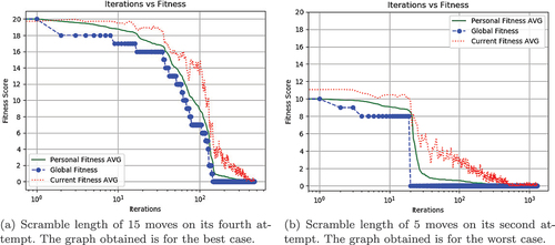
Figures 1 shows the Iteration vs Fitness graph obtained for PSO. The Y-axis shows the fitness score and the X-axis shows the number of iterations, which is on a semi-log scale. Figure 1a is for the best case where the average iteration it takes for the next particle to find the solved state is minimum (6.5). If the average iteration between the particles to find the solved state is minimum, then the PSO algorithm finishes its execution much faster. Figure 1b is for the worst case where the average iteration it takes for the next particle to find the solved state is maximum (25.42). If the average iteration between the particles to find the solved state is large, then the PSO algorithm will take a longer time to finish its execution.

Figure 1. Iteration vs Fitness graph of PSO.

Greedy Algorithm

A greedy algorithm is an algorithm that tries to solve an optimization problem by selecting the local optimum solution at each stage of the problem. These algorithms will sometimes find the global optimum solutions to the problem, but sometimes they can come up with solutions near the global optimum or worse than the global optimum. This is because selecting a local optimum solution at each stage may not guarantee that they lead to the global best solution. An example of a greedy algorithm is Dijkstra’s algorithm, which is used for finding the shortest path between nodes in a graph (Dijkstra 1959).

Greedy Tree Search Algorithm for Solving the Rubik’s Cube

The greedy tree search algorithm applies moves that reduce the fitness at each depth. From any state of the Rubik’s cube, eighteen moves can be applied to it. These eighteen moves can take the cube from the current state to eighteen new states. If any of these states have a fitness value less than the previous state, then the move that gives the minimum fitness is applied to the cube. This move selection method decreases the fitness value at each depth.

If the next eighteen moves do not lead to a state with a fitness value less than the previous state, then the last applied move is undone and a move that gives the next minimum fitness value is applied to the cube. This stage is called backtracking.

Cycles occur when a previously reached state is encountered again and the move to be applied from this state is the same move that was applied when this state was previously encountered. Since a greedy approach is used when selecting the next move to be applied to the cube, the algorithm can apply the same move that it previously applied when it first encountered that state, causing the algorithm to go through a cyclic loop and never reach the solved state. Cycles can be prevented by checking if the next move to be applied to the cube will make it reach a state that has been encountered before. If this state has been encountered before, then this move will not be applied to the cube and the next move is applied.

Number of Function Evaluations

The greedy algorithm runs for $N$ iteration. During each iteration, the algorithm applies each of the 18 possible moves to the cube, and the cube will reach 18 different states from the current state. The algorithm checks the fitness of these 18 states using Equation 2(2) $F(S(t))=\frac{1}{n}\sum _{i=1}^{n}Kociemba(S(t{)}_i)$(2) and selects the move that takes the cube to a state whose fitness value is less than or equal to the current state. The Kociemba’s algorithm is called $n$ times for the 18 different states that are reachable from the current state. Therefore, the total number of function evaluations is $n\times 18\times N=18nN$.

Kociemba’s algorithm is not called during the detection of a cycle since the algorithm only checks if the move that gives the minimum fitness value takes the cube to a state that has already been visited.

The algorithm does not evaluate the fitness of the cube states during backtracking. In the backtracking stage, the algorithm goes back to the previous depth and undo the last move applied to the cube. Then it applies the move which gives the next minimum fitness value. The move that gives the next minimum fitness value has already been found during the previous iterations.

Observations

Table 2 shows the observations obtained for the greedy tree search. The algorithm ran for 10,000 iterations. Length shows the length of the scramble that was applied to the cube. % out of five attempts how many attempts were successful. Actual shows the length of the solution predicted by Kociemba’s algorithm. Obtained shows the length of the solution given by the greedy tree search. MinFit shows the minimum fitness value found by the program. If the cube is solved then the minimum fitness is zero. MaxDeep tells us the maximum depth that the algorithm went to find the solution. Iterations shows the total iterations it took to solve the cube. NFE shows the total number of times the evaluation function was called.

Table 2. Observations for greedy tree search algorithm.

Length	%	Actual	Obtained	MinFit	MaxDeep	Iterations	NFE
5	5/5	9	5	0	5	5	270
		8	5	0	5	5	270
		5	5	0	5	5	270
		5	5	0	5	5	270
		13	11	0	11	13	702
10	5/5	19	15	0	15	201	10854
		19	12	0	15	26	1404
		18	18	0	18	18	972
		14	10	0	10	10	540
		14	10	0	10	10	540
15	4/5	20	22	0	22	22	1188
		20	25	0	25	25	1350
		18	NA(18)	12	23	10000	540000
		15	27	0	27	1633	88182
		20	15	0	15	15	810
20	3/5	19	NA(23)	11	31	10000	540000
		20	NA(12)	10	26	10000	540000
		20	20	0	20	20	1080
		19	22	0	22	22	1188
		20	27	0	27	184	9936
25	5/5	20	24	0	24	65	3510
		19	22	0	22	22	1188
		20	31	0	32	815	44010
		20	20	0	20	20	1080
		20	19	0	19	19	1026
30	4/5	20	21	0	21	35	1890
		20	29	0	29	634	34236
		21	NA(40)	12	46	10000	540000
		20	20	0	20	38	2052
		20	19	0	19	19	1026

In the column Obtained a value is of the form NA(18). This means that the solution was not found and when the program stopped its execution after 10,000 iterations it gave a solution of length 18 which would not completely solve the cube. In the column MinFit for the scramble length of 15 in its third row, the cube is not solved and the minimum fitness is 12. This means that the cube is 12 moves away from the solved state when the program is terminated.

From this table, by taking the average of the obtained solution length, the number of iterations, and the number of function evaluations for each scramble length, the greedy tree search algorithm solves the Rubik’s cube with an average of 6 to 23 moves. The average number of iterations is around 6 to 4050, and the evaluation function is called on average 356 to 218,440 times.

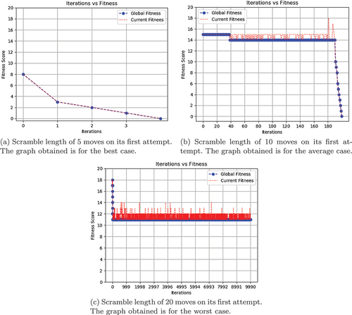
Figures 2 shows how the fitness value of the cube changes with every iteration and also the change in the global minimum value with every iteration. Figure 2a is for the best case where the global minimum value decreases with each iteration along with the current fitness. Figure 2b, is for the average case. In the average case, the solution to the cube is found, but the algorithm did a few backtracking along the way. This is indicated by the spikes in the red plot which indicates the current fitness during each iteration. Figure 2c, is for the worst cases where the solution to the cube could not be found and the minimum fitness reached is greater than 0.

Figure 2. Iteration vs Fitness graph of greedy tree search.

Ant Colony Optimization

Ant colony optimization (ACO) algorithm is a metaheuristic optimization algorithm which is a probabilistic technique used for solving problems that are reducible to finding good paths through graphs (Dorigo 1991; Dorigo, Birattari, and Stutzle 2006). The algorithm takes inspiration from the behavior of biological ants. To find the food source, the ants leave behind a pheromone trail from the starting location to the food source. The pheromone trail helps the ants to determine how far or near the food source is. If the food source is near, the ants will leave behind more pheromones, or else the amount of pheromones deposited is less.

The pheromone deposited by an ant $k$, on an edge $(i,j)$ is calculated using Equation 8.(8) $\mathrm{\Delta }{\tau }_{i,j}^k=\left\{\begin{array}{c}\frac{1}{L_k},where{k}^{th}anttraversededge(i,j)\\ 0,otherwise\end{array}\right.$(8)

(8) $\mathrm{\Delta }{\tau }_{i,j}^k=\left\{\begin{array}{c}\frac{1}{L_k},where{k}^{th}anttraversededge(i,j)\\ 0,otherwise\end{array}\right.$(8)

This means that if an ant $k$ travels from node $i$ to node $j$ of a graph then it will deposit some amount of pheromone represented by $\mathrm{\Delta }{\tau }_{i,j}^k$, which is equal to $\frac{1}{L_k}$ where $L_k$ is the length of the path, distance from node $i$ to node $j$, found by the ant $k$. If the path length is more, then the pheromone level deposited will be less.

The total amount of pheromones deposited is the sum total of the pheromones deposited by all the ants that traversed the edge $(i,j)$, is calculated using Equation 9(9) ${\tau }_{i,j}={\mathrm{\Sigma }}_{k=1}^m\mathrm{\Delta }{\tau }_{i,j}^k$(9) ,

(9) ${\tau }_{i,j}={\mathrm{\Sigma }}_{k=1}^m\mathrm{\Delta }{\tau }_{i,j}^k$(9)

where $m$ represents the total number of ants that traversed the edge $(i,j)$. To decrease the amount of pheromone deposited after each iteration an evaporation constant $p$ is introduced and Equation 9(9) ${\tau }_{i,j}={\mathrm{\Sigma }}_{k=1}^m\mathrm{\Delta }{\tau }_{i,j}^k$(9) changes to Equation 10.(10) ${\tau }_{i,j}=(1-p){\tau }_{i,j}+{\mathrm{\Sigma }}_{k=1}^m\mathrm{\Delta }{\tau }_{i,j}^k$(10)

(10) ${\tau }_{i,j}=(1-p){\tau }_{i,j}+{\mathrm{\Sigma }}_{k=1}^m\mathrm{\Delta }{\tau }_{i,j}^k$(10)

The probability of selecting an edge is calculated using Equation 11(11) $P_{i,j}=\frac{{({\tau }_{i,j})}^{\alpha }{({\eta }_{i,j})}^{\beta }}{{\mathrm{\Sigma }}_{alledges}{({\tau }_{i,j})}^{\alpha }{({\eta }_{i,j})}^{\beta }}$(11) ,

(11) $P_{i,j}=\frac{{({\tau }_{i,j})}^{\alpha }{({\eta }_{i,j})}^{\beta }}{{\mathrm{\Sigma }}_{alledges}{({\tau }_{i,j})}^{\alpha }{({\eta }_{i,j})}^{\beta }}$(11)

where $\alpha$ is a parameter that is used to control the relative weight of the total amount pheromones deposited on an edge $(i,j)$ represented by ${\tau }_{i,j}$ and $\beta$ is a parameter that is used to control the relative weight of the heuristic value ${\eta }_{i,j}$, which is computed using Equation 12.(12) ${\eta }_{i,j}=\frac{1}{L_k}$(12)

(12) ${\eta }_{i,j}=\frac{1}{L_k}$(12)

For example if an ant wants to select an edge from one of the three edges $a$, $b$, and $c$ then using the above equations (Equations 8(8) $\mathrm{\Delta }{\tau }_{i,j}^k=\left\{\begin{array}{c}\frac{1}{L_k},where{k}^{th}anttraversededge(i,j)\\ 0,otherwise\end{array}\right.$(8) - 11(11) $P_{i,j}=\frac{{({\tau }_{i,j})}^{\alpha }{({\eta }_{i,j})}^{\beta }}{{\mathrm{\Sigma }}_{alledges}{({\tau }_{i,j})}^{\alpha }{({\eta }_{i,j})}^{\beta }}$(11) ) the probability of selecting the three edges are calculated and found to be as follows, $P=[0.76,0.19,0.05]$. Now the cumulative sum is calculated as $Cumulative\mathrm{\_}Sum=[0.76+0.19+0.05,0.19+0.05,0.05]=[1,0.24,0.05]$. A random number $r$ is generated and is between the range $[0,1]$. If $0.24\le r\le 1.00$ node $a$ is selected, if $0.05\le r\le 0.24$ node $b$ is selected and if $0.00\le r\le 0.05$ node $c$ is selected. This method of selecting the edge is called as roulette wheel selection Lipowski and Lipowska (2012).

Ant Colony Optimization for Solving the Rubik’s Cube

ACO is suitable for solving the Rubik’s cube since it is used for solving graph-based problems. For the ACO to completely solve the cube, a few optimizations are made to it.

The pheromone deposited by an ant $k$, on an edge $(i,j)$ is given by Equation 8.(8) $\mathrm{\Delta }{\tau }_{i,j}^k=\left\{\begin{array}{c}\frac{1}{L_k},where{k}^{th}anttraversededge(i,j)\\ 0,otherwise\end{array}\right.$(8) This means that if an ant $k$ travels from node $i$ to node $j$ then it will deposit some amount of pheromone represented by $\mathrm{\Delta }{\tau }_{i,j}^k$ which is equal to $\frac{1}{L_k}$, where $L_k$ is the length of the path between node $i$ and node $j$ found by the ant $k$. In the context of a Rubik’s cube, the length of the path is the distance from the current state of the cube to the solved state. If an ant $k$ applies a move $R$ to the cube from state $S$ then it will go to the state $S+R$. The state $S+R$ will have a fitness value, which is the number of moves needed to solve the cube from the state $S+R$ given by Kociemba’s algorithm which is calculated using Equation 2.(2) $F(S(t))=\frac{1}{n}\sum _{i=1}^{n}Kociemba(S(t{)}_i)$(2)

For the Rubik’s Cube, $i$ represents the current state of the cube $S$ and $j$ represents the next state of the cube which can be reached by applying any of the possible moves in ${\mathbb{M}}_{HTM}=$ {R, R,’ R2, L, L,’ L2, F, F,’ F2, B, B,’ B2, U, U,’ U2, D, D,’ D2} to the cube from the state $S$. Let M be a singleton set with only a single element and this element can be any one of the possible eighteen moves that can be applied to the cube. Equation 13(13) $\mathrm{\Delta }{\tau }_{S,\left(S+\mathbb{M}\right)}^k=\left\{\begin{array}{cc}\frac{1}{F\left(S+\mathbb{M}\right)}& ,where{k}^{th}anttraversedtheedge\left(S,S+\mathbb{M}\right)\\ 0& ,otherwise\end{array}\right.$(13) calculates the pheromone deposited by the ant $k$ that traversed the edge between the state $S$ and $(S+\mathbb{M})$ of the cube.

(13) $\mathrm{\Delta }{\tau }_{S,\left(S+\mathbb{M}\right)}^k=\left\{\begin{array}{cc}\frac{1}{F\left(S+\mathbb{M}\right)}& ,where{k}^{th}anttraversedtheedge\left(S,S+\mathbb{M}\right)\\ 0& ,otherwise\end{array}\right.$(13)

Now the total amount of pheromones deposited is the sum total of the pheromones deposited by all the ants that traversed the edge between the state $S$ and $\left(S+\mathbb{M}\right)$ calculated using Equation 14,(14) ${\tau }_{S,(S+\mathbb{M})}={\mathrm{\Sigma }}_{k=1}^m\mathrm{\Delta }{\tau }_{S,(S+\mathbb{M})}^k$(14)

(14) ${\tau }_{S,(S+\mathbb{M})}={\mathrm{\Sigma }}_{k=1}^m\mathrm{\Delta }{\tau }_{S,(S+\mathbb{M})}^k$(14)

where $m$ is the total number of ants that traversed the edge between state $S$ and state $\left(S+\mathbb{M}\right)$. The probability of selecting an edge is given by Equation 15(15) $P_{S,(S+\mathbb{M})}=\frac{{({\tau }_{S,(S+\mathbb{M})})}^{\alpha }{({\eta }_{S,(S+\mathbb{M})})}^{\beta }}{{\mathrm{\Sigma }}_{alledges}{({\tau }_{S,(S+\mathbb{M})})}^{\alpha }{({\eta }_{S,(S+\mathbb{M})})}^{\beta }}$(15) ,

(15) $P_{S,(S+\mathbb{M})}=\frac{{({\tau }_{S,(S+\mathbb{M})})}^{\alpha }{({\eta }_{S,(S+\mathbb{M})})}^{\beta }}{{\mathrm{\Sigma }}_{alledges}{({\tau }_{S,(S+\mathbb{M})})}^{\alpha }{({\eta }_{S,(S+\mathbb{M})})}^{\beta }}$(15)

where ${\eta }_{S,\left(S+\mathbb{M}\right)}$ is calculated using Equation 16(16) ${\eta }_{S,(S+\mathbb{M})}=\frac{1}{F(S+\mathbb{M})}$(16) as follows:

(16) ${\eta }_{S,(S+\mathbb{M})}=\frac{1}{F(S+\mathbb{M})}$(16)

The roulette wheel technique is used for selecting the edge after the probability of each edge is computed. In the original ACO algorithm proposed by Dorigo Dorigo (1991), the value of $\alpha$ and $\beta$ are set to 1 and 5, respectively. Through experimental analysis, it was found that the values of $\alpha$ and $\beta$ of 1 and 5 did not affect the performance of the ACO algorithm when it comes to solving the Rubik’s cube. Since the values of $\alpha$ and $\beta$ do not affect the performance, they are set to 1.

Assumptions

Some assumptions are made before the algorithm begins its execution. If there are $n$ ants that need to search the Rubik’s cube search tree, then each ant will start traversing the depth of the tree one after the other. The ants follow the pheromone trail left by the previous ants. The ants select an edge based on the probability which is determined by the pheromone values left by the ants that traversed the tree before the current ant. For the first ant that is about to traverse the tree, no ant has traversed the tree before it and the pheromone trail is 0.

The probability becomes undefined when inserting 0 in Equation 15.(15) $P_{S,(S+\mathbb{M})}=\frac{{({\tau }_{S,(S+\mathbb{M})})}^{\alpha }{({\eta }_{S,(S+\mathbb{M})})}^{\beta }}{{\mathrm{\Sigma }}_{alledges}{({\tau }_{S,(S+\mathbb{M})})}^{\alpha }{({\eta }_{S,(S+\mathbb{M})})}^{\beta }}$(15) To prevent this, an assumption is made that an ant has traversed the entire tree of possibilities for the Rubik’s cube and has deposited a pheromone value of 0.000001 at every branch of the tree. This value is small but not 0. It ensures that the probability value does not become undefined. This is done for the proper implementation of the algorithm.

Equation 13(13) $\mathrm{\Delta }{\tau }_{S,\left(S+\mathbb{M}\right)}^k=\left\{\begin{array}{cc}\frac{1}{F\left(S+\mathbb{M}\right)}& ,where{k}^{th}anttraversedtheedge\left(S,S+\mathbb{M}\right)\\ 0& ,otherwise\end{array}\right.$(13) is used to determine the amount of pheromones to be deposited on an edge between the state $S$ and $\left(S+\mathbb{M}\right)$ traversed by an ant $k$. If the state $\left(S+\mathbb{M}\right)$ is solved, then the fitness value of the solved state is 0. If the fitness value of the state $\left(S+\mathbb{M}\right)$ is 0, then from Equation 13(13) $\mathrm{\Delta }{\tau }_{S,\left(S+\mathbb{M}\right)}^k=\left\{\begin{array}{cc}\frac{1}{F\left(S+\mathbb{M}\right)}& ,where{k}^{th}anttraversedtheedge\left(S,S+\mathbb{M}\right)\\ 0& ,otherwise\end{array}\right.$(13) , the amount of pheromones to be deposited becomes undefined.

To prevent this, when the cube is solved the amount of pheromones to be deposited is set to a value of 9,999,999. This is done for proper implementation of the algorithm and to avoid division by zero errors.

Pheromone Dictionary

In ACO, a pheromone matrix, similar to the adjacency matrix of a graph, is used to represent the amount of pheromone between the nodes of the graph. For solving the Rubik’s cube a pheromone dictionary is used instead of a pheromone matrix. The pheromone values for an edge will be stored in the pheromone dictionary. The keys represent the state of the Rubik’s cube, and the value will be a list of key-value pairs that show the pheromone value at each edge from the current state.

Depth Traversed and Regrouping

Since the ants will try to find the solution to the Rubik’s cube by searching each depth of the tree, there should be some way to ensure that they do not get scattered in the search space. A regrouping strategy regroups the ants to a common node if the following conditions are satisfied.

1. An ant has found a state whose fitness is less than the global minimum. Then all the ants will regroup in this new state.

2. All ants have searched till a certain depth, which is equal to the global minimum value, and if no ant has found a state whose fitness is less than the global minimum, then they will regroup from the starting state and try again.

When the ants regroup back to the starting state when a new global minimum value could not be found, the pheromone value of all the edges of the states that were found after the starting state will be set back to 0.000001. All the new state entries in the pheromone dictionary which were found after the starting state will be removed. This ensures that the ants can try again and won’t get lost in the search space due to pheromones left behind during the previous iteration.

Number of Function Evaluations

In ACO, the move to be applied to the cube is determined by assigning a probability value to each of the eighteen moves and using the roulette wheel technique to select one of the eighteen moves.

The probability value of a move is determined using Equation 15(15) $P_{S,(S+\mathbb{M})}=\frac{{({\tau }_{S,(S+\mathbb{M})})}^{\alpha }{({\eta }_{S,(S+\mathbb{M})})}^{\beta }}{{\mathrm{\Sigma }}_{alledges}{({\tau }_{S,(S+\mathbb{M})})}^{\alpha }{({\eta }_{S,(S+\mathbb{M})})}^{\beta }}$(15) , for which four values are needed. The first is the total amount of pheromones deposited on the edge, which is the sum of the pheromones deposited by the ants that traversed that edge. The second value is the fitness of the edge, which is the fitness value of the state obtained when that move is applied to the cube. The third value is the fitness of the adjacent edges. For example, the edges adjacent to the edge R, are the moves that can be applied to the cube after applying the move R. An edge has eighteen adjacent edges since eighteen moves can be applied from any cube position. The fourth value is the total amount of pheromones deposited by the ants that traversed those adjacent edges.

The evaluation function (Kociemba’s algorithm) is first called to calculate the fitness value of the current edge. Then it called to calculate the fitness value of the eighteen adjacent edges. To calculate the probability of a single move the evaluation function is called a total of nineteen times.

The probability value is computed for all eighteen moves that can be applied from the current cube state. The Kociemba’s algorithm is called a total of $19\times 18=342$ times. This is done by all $P$ ants for each iteration $N$. As explained in Section 1.5 the Kociemba’s algorithm is called $n$ times for a single cube state. Therefore ACO calls Kociemba’s algorithm $342\times n\times N\times P=342nNP$ times.

Observations

For the experimental analysis of PSO (Section 3.3), the number of particles is 50 and the number of iterations is 10,000. This is to ensure that the cube gets solved by covering a large number of states with a large number of particles and also to ensure that the particles have time to cover a large number of states with a large number of iterations. The ACO takes more time to go through one iteration with 50 ants compared to one iteration with 50 particles in PSO. Therefore, the number of ants is reduced to 25 and the number of iterations is reduced to 100.

If $n$, the number of times Kociemba’s algorithm gets called for a cube state, is set to a value of 3, ACO takes a very long time to find the solution. A single iteration with 25 ants takes at least 1 hour to complete for 5 move scrambles and more than 5 hours for 15 move scrambles. This is because when $n$ has the value 3 Kociemba’s algorithm gets called $342\times 3\times N\times P=1026NP$ times. Therefore, $n$ is set to a value of 1 only for ACO to do its analysis.

The columns of Table 3 are the same as that of Table 1. For the scramble length of 15 moves on its $4^{th}$ attempt, its row has the value TLE – Time Limit Exceeded. This is because ACO takes a long time to find the solution. After 12 hours, it completed only 8 iterations and the fitness obtained was around 20. From this, it became clear that ACO would take days to solve the cube and the execution was stopped since there is no point in running the ACO algorithm for days to solve the cube.

Table 3. Observations for ant colony optimization algorithm.

Length	%	Actual	Obtained	First	Last	Average	NFE	Total
5	5/5	14	6	5	6	0.04	51300	25
		5	5	4	5	0.04	42750	25
		5	8	7	8	0.04	68400	25
		5	5	4	5	0.04	42750	25
		12	5	12	13	0.04	111150	25
10	5/5	14	10	9	10	0.04	85500	25
		10	10	9	10	0.04	85500	25
		10	10	9	10	0.04	85500	25
		10	10	9	10	0.04	85500	25
		18	10	9	10	0.04	85500	25
15	4/5	19	19	18	19	0.04	162450	25
		19	17	16	17	0.04	145350	25
		16	16	15	16	0.04	136800	25
		TLE	TLE	TLE	TLE	TLE	TLE	TLE
		20	20	19	20	0.04	171000	25

Similarly, the analysis for the scrambles of lengths 20, 25, and 30 moves using ACO is not done. For these scrambles, the ACO algorithm took around 15 hours to complete 25 iterations. From this, it became clear that the ACO algorithm would take days to complete the execution for scrambles of length greater than 20 moves.

From this table, the ACO algorithm solves the Rubik’s cube with an average of 6 to 18 moves. The average number of iterations it takes to solve the cube is around 7 to 18 iterations. The evaluation function is called on average 63,300 to 154,000 times. The ACO is only suitable for solving the Rubik’s cube when the scramble length is less than 15 moves, and when ACO is used for solving the cube, the Kociemba’s algorithm must be called only once for the cube state. Increasing the number of times the cube state is to be evaluated by Kociemba’s algorithm affects the performance of the ACO.

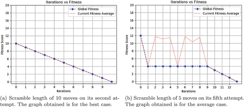
Figure 3a shows how one of the ants finds the next minimum fitness in the current iteration and all the ants will regroup to the state that gave the minimum fitness in the next iteration. This continues for all the iterations and the fitness will decrease after each iteration. Figure 3b shows how the ants regroup to the point where the minimum fitness was found if the new minimum fitness could not be found after a certain number of iterations. Here the ants regroup to the state that gave the global minimum fitness after 4 iterations and then regroup again after 4 iterations. In the worst case, the ACO would not be able to solve the cube within the specified number of iterations or within a specified time limit.

Figure 3. Iteration vs Fitness graph of ACO.

Krill Herd Optimization

Krill herd optimization (KHO) is a swarm intelligence algorithm that simulates the herding behavior of krill individuals to solve optimization problems (Gandomi and Alavi 2012). To solve the Rubik’s cube a variation of KHO called discrete krill herd optimization algorithm (DKHO) is used that solves problems in the discrete search domain (Sur and Shukla 2014). The original DKHO proposed is used for optimizing graph-based network routes. Optimizations are made to the original DKHO algorithm for it to solve the Rubik’s cube.

Krill Herd Optimization for Solving the Rubik’s Cube

The DKHO algorithm for solving the Rubik’s cube has four stages.

Move Selection

In the move selection stage, the krills must decide which move they must apply to the cube, from the current state to reach the next state. The krills select the move based on two methods. One is the greedy move selection method and the other is the probability move selection method.

In the greedy move selection method, the krill will select the move that gives a fitness value that is less than the fitness of the current state. This move selection is the same as the one used by the greedy tree search algorithm explained in Section 4.1.

In probability move selection, each krill will assign probability values for each move and, the roulette wheel technique is used for selecting the move. This is similar to the move selection method used by the ACO algorithm (Section 5.1). Since there is no concept of pheromone trail like in the ACO algorithm, the probability is calculated using Equation 17(17) $P_{S,(S+\mathbb{M})}=\frac{({\eta }_{S,(S+\mathbb{M})})}{{\mathrm{\Sigma }}_{alledges}({\eta }_{S,(S+\mathbb{M})})}$(17) as follows:

(17) $P_{S,(S+\mathbb{M})}=\frac{({\eta }_{S,(S+\mathbb{M})})}{{\mathrm{\Sigma }}_{alledges}({\eta }_{S,(S+\mathbb{M})})}$(17)

where ${\eta }_{S,\left(S+\mathbb{M}\right)}$ is calculated using Equation 16(16) ${\eta }_{S,(S+\mathbb{M})}=\frac{1}{F(S+\mathbb{M})}$(16) (Section 5.1).

Selecting a move by computing its probability is done when the greedy method cannot find a move whose fitness value is less than the fitness value of the current state.

When the cube is solved, its fitness value is 0. Therefore ${\eta }_{S,\left(S+\mathbb{M}\right)}$ becomes $1/0=Undefined$. To prevent division by zero error, when the fitness of the cube is 0, ${\eta }_{S,\left(S+\mathbb{M}\right)}$ is set to a value of 9,999,999.

Killing of Unfit Krills

This stage occurs after all the krills have selected a move to apply to the cube. All the unfit krills are killed in this stage. A krill is said to be unfit if its fitness value is greater than a threshold value. The threshold value is calculated using Equation 18(18) $threshold=1.5\times globalMinimum$(18) as follows:

(18) $threshold=1.5\times globalMinimum$(18)

where the $globalMinimum$ is the global minimum fitness value of the current iteration. The threshold value is 50% greater than the global minimum value. If the range of values that are said to be fit is too small then there is a chance that many of the krills will be killed off, and only one krill will survive. This can cause problems in the reproduction stage as there would not be enough krill to do reproduction to bring the population back to normal. If the range of values that are said to be fit is too high then no krill will get killed, and this can cause many of the krills to wander around in the search space without finding the solution, which can slow down the time needed to find the solved state.

Reproduction

After the killing stage, the remaining krills will do reproduction till the population is back to normal. For the remaining krills to do reproduction, they need to have some sort of genetic information that they can pass onto their offsprings. In the context of the Rubik’s cube, the genetic information is the move sequence that the krill has applied to the cube. The children are produced by cutting the move sequence of the parents at a random point and swapping the tail of both the move sequences.

Mutation

Mutation happens after the reproduction stage and mutation is done to the offsprings that are not fit, to improve their fitness. The mutation is done by taking the move sequence of the unfit krill and replacing a few random moves in the move sequence with randomly selected moves from the set $M_{HTM}$. For example, if an unfit krill has the move sequence L, R, D, U, F, B2, then the mutation is done by taking a few random moves in the sequence, for example, R, U, and F, and replacing them with randomly selected moves from the set $M_{HTM}$. If the randomly selected moves from the set $M_{HTM}$ are F, B, and R2, then the new sequence becomes L, F, D, B, R2, B2.

Number of Function Evaluations

The number of times the evaluation function (Kociemba’s algorithm) gets called varies for DKHO, unlike PSO, greedy, and ACO. The number of times the Kociemba’s algorithm gets called for PSO, greedy, and ACO are $nNP$, $18nN$, and $342nNP$, respectively. The number of times Kociemba’s algorithm gets called can vary according to the scramble length, and it also depends on whether or not the DKHO went through each of its different stages – move selection, killing of unfit krills, reproduction, and mutation stage.

In the move selection stage, the krills must decide which move to apply to the cube. This is decided by using one of the two methods – the greedy method and the probability-based method. In the greedy method, the krills will select the move that takes the cube to the state whose fitness is less than the fitness of the current state. If the krill cannot find such a move, then the krill will assign a probability value to each of the moves and use a roulette wheel to decide which move is to be selected. The krills always uses the greedy move selection first. If the greedy method cannot find a suitable move then it uses the probability-based move selection.

In the greedy method, the krill needs to find the fitness of the eighteen states that are reachable from the current state. Therefore it needs to call Kociemba’s algorithm eighteen times to determine the fitness of those eighteen states. Since Kociemba’s algorithm gets called $n$ times for a single state, the number of times it gets called in greedy move selection is $18n$. This is done by $P$ krills for each iteration $n$. Therefore, the total number of times Kociemba’s gets called is $18nNP$.

For probability-based move selection, to calculate the probability of a move, the krill needs to find the fitness of the state that can be reached from the current state and also the fitness of the states that can be reached from the next state. For example, to determine the probability value of the move R, the krill needs to find the fitness of the state reached by applying the move $R$ to the cube, which is $S+R$. It then needs to find the fitness of the eighteen states that can be reached from the state $S+R$. Therefore, Kociemba’s algorithm gets called a total of 19 times for a single move. Since eighteen moves can be applied to the cube, Kociemba’s algorithm gets called $19\times 18=342$ times. Kociemba’s algorithm gets called $n$ times for a single cube state. Therefore it is called a total of $342n$ times when probability move selection is used. This is done by $P$ krills for each iteration $N$. Here, the total number of times Kociemba’s algorithm gets called is $342nNP$.

In the killing stage, krills having a fitness value greater than the threshold value are killed since they are unfit. The fitness value of the krills is computed when the move is applied to the cube in the move selection stage, and it would not be computed again in the killing stage. The Kociemba’s algorithm do not get called in the killing stage.

In the reproduction stage, the remaining krills will do reproduction to bring the population back to normal. In the worst-case, out of the $P$ krills, only two krills are left. If only one krill is left then reproduction would not happen with only a single krill. The two krills reproduce till the population is back to $P$. In this stage, Kociemba’s algorithm is used to evaluate the fitness of the new krills. When only two krills are left then they will do reproduction till they get $P-2$ offspring. So the Kociemba’s algorithm gets called at most $P-2$ times in the reproduction stage. Kociemba’s algorithm is called $n$ times for a cube state, which brings the total number of function calls to $n(P-2)$. This is done for each iteration $N$. Therefore, the total number of times Kociemba’s algorithm gets called is $Nn(P-2)$.

In the mutation stage, the krills born in the reproduction stage that are unfit, whose fitness is less than the threshold value, are mutated to improve their fitness. In the worst case, all the $P-2$ krills born in the reproduction stage are unfit. So all the $P-2$ krills have to be mutated to improve their fitness. In this stage, Kociemba’s algorithm gets called a total of $P-2$ times. Kociemba’s is called a total of $n$ times for a single cube state which brings the total number of function evaluations to $n(P-2)$. This is done for each iteration $N$. Therefore, the total number of times Kociemba’s algorithm gets called is $Nn(P-2)$.

In the best case, the krills undergo only the move selection stage and do not undergo killing, reproduction, and mutation stages. In the move selection stage, all the krills use only the greedy method for selecting the move and not the probability method. When this happens, the fitness decrease after each iteration for all the krills. In the best-case scenario, since only the greedy method is used for selecting the move and since it does not undergo killing, reproduction, and mutation stages, the number of times the evaluation function gets called is $18nNP$.

In the worst-case, the krills go through all four stages and Kociemba’s algorithm is called during each stage. In the move selection stage, in the worst-case, the krills first uses the greedy method for selecting the move but do not find a move that gives a fitness value less than the fitness value of the current state. When this happens, it uses the probability method for selecting a move. When it uses both methods the number of times Kociemba’s algorithm gets called is $18nNP+342nNP$, which is the sum of the total of the number of times it gets called for the greedy method and the probability method.

In the worst case, the total number of times Kociemba’s algorithm gets called is the sum of the total of the times it gets called during each stage of the algorithm. This is given by Equation 19(19) $=nN(362P-4)$(19) which can be calculated using as follows:

$=18nNP+342nNP+0+nN(P-2)+nN(P-2)$

$=360nNP+nNP+nNP-2nN-2nN$

$=362nNP-4nN$

(19) $=nN(362P-4)$(19)

For DKHO, the number of times Kociemba’s algorithm gets called is $18nNP$ times for the best case and $nN(362P-4)$ times for the worst case.

Observations

The DKHO algorithm for solving the Rubik’s cube takes more time to go through one iteration with 50 krills compared to 50 particles in PSO. Therefore, the number of krills is reduced to 25 and the number of iterations is reduced to 100.

The columns for Table 4 is the same as that of Table 1 and Table 3. For some scrambles, their rows have the value TLE – Time Limit Exceeded. It is because DKHO takes a long time to find the solution, just like the ACO. So the execution was stopped for those scrambles. Similarly, the analysis for scrambles of lengths 25 and 30 moves was not done, because the algorithm took an hour to complete one iteration.

Table 4. Observations for discrete krill herd optimization algorithm.

Length	%	Actual	Obtained	First	Last	Average	NFE	Total
5	5/5	5	5	4	4	0	6750	25
		5	5	4	4	0	6750	25
		10	10	9	9	0	13500	25
		5	5	4	4	0	6750	25
		10	6	5	5	0	8100	25
10	4/5	TLE	TLE	TLE	TLE	TLE	TLE	TLE
		10	10	9	9	0	13500	25
		11	11	10	10	0	14850	25
		10	10	9	9	0	13500	25
		12	12	11	11	0	16200	25
15	2/5	TLE	TLE	TLE	TLE	TLE	TLE	TLE
		20	18	17	17	0	30468	25
		TLE	TLE	TLE	TLE	TLE	TLE	TLE
		TLE	TLE	TLE	TLE	TLE	TLE	TLE
		19	18	17	17	0	24300	25
20	1/5	TLE	TLE	TLE	TLE	TLE	TLE	TLE
		TLE	TLE	TLE	TLE	TLE	TLE	TLE
		TLE	TLE	TLE	TLE	TLE	TLE	TLE
		TLE	TLE	TLE	TLE	TLE	TLE	TLE
		19	19	18	18	0	25650	25

The performance of DKHO depends on the scramble length and the number of times Kociemba’s algorithm gets called to evaluate the cube state, which is $n$.

When the scramble length is less than 10 moves, the krills use the greedy method to select the move. This is because there is a high chance of finding a move that takes the cube to a state whose fitness value is less than the fitness of the current state. The cube is nearer to the solved state when the scramble length is less than 10 moves. When the greedy method is used, the number of times Kociemba’s algorithm gets called is $18nNP$. If the value of $n$ is 3 then Kociemba’s algorithm gets called $18\times 3\times N\times P=54NP$ times. Therefore, the DKHO can solve the cube when the scramble length is less than 10 moves and when $n$ has a value of 3.

For scramble length greater than 10 moves, the krills use the probability method to select a move. This is because there is a low chance of finding a move that takes the cube to a state which has a fitness value less than the fitness of the current state. This is because the cube is farther away from the solved state. When the probability method is used, the number of times Kociemba’s algorithm gets called is $18nNP+342nNP$. If the value of $n$ is 3 then Kociemba’s algorithm gets called $(18\times 3\times N\times P)+(342\times 3\times N\times P)=1080NP$ times. Due to this reason, the DKHO takes a long time to find the solved state for scramble length greater than 10 moves. For the attempts when the DKHO could solve the cube when scramble length is greater than 10 moves (for scramble length of 20 moves on its fifth attempt), the greedy method is used rather than the probability-based move selection.

For DKHO, the value of $n$ should be set to 1 so that, it can solve the cube when the scramble length is greater than 15 moves in a reasonable amount of time.

From this table, the DKHO algorithm solves the Rubik’s cube with an average of 6 to 18 moves. The average number of iterations it takes to solve the cube is around 5 to 17 iterations. The evaluation function is called on average 8400 to 27,400 times.

In Figure 4a, each krill finds the next minimum fitness after each iteration. The fitness of every krill will decrease after each iteration and the cube gets solved after a certain number of iterations. These kinds of graphs are obtained for scrambles less than 10 moves long and the type of edge selection method used by the krill is the greedy approach. Since the greedy approach is used each krill will have the same fitness value.

Figure 4. Iteration vs Fitness graph of KHO.

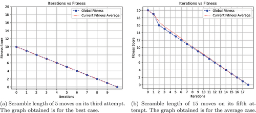
In Figure 4b, the krills spread out to find the solved state. It happens for scrambles of length 10 moves and above. It happens when the greedy method does not work because the fitness value at the next depth will be the same or will be greater than the current fitness. So the krills will use the probability method to select a move. This can cause the krills to select different moves causing them to follow different paths rather than the same path. In the worst case, the DKHO cannot solve the cube within the specified number of iterations or within a specified time limit.

Experimental Analysis

Experimental Setup

To find out which of the above-described algorithms will give the optimum solution in the optimum amount of time, each algorithm is given scrambles of three difficulty levels. One is an easy scramble which is five moves long, the next is a medium scramble which is fifteen moves long, and the last one is a hard scramble which is twenty-five moves long. Each algorithm will be given three different scrambles for each difficulty level. The scrambles used are shown in Table 5. These scrambles have been generated randomly.⁷

Table 5. Scrambles used for comparative analysis of the algorithms.

Length	Scramble
5	F2 L D2 B2 F
	B U’ R2 B F’
	R2 B2 D F R2
15	U D2 F’ U2 R’ B2 L D’ F2 U2 B2 R’ F2 U L’
	D B L U B L2 U2 F’ R’ L’ D2 R2 F U2 L’
	B2 L2 U B F2 D’ U’ R2 D B’ U F’ R’ B’ L
25	L2 D2 U’ L2 F’ R’ U’ F’ R2 L U2 R2 F’ U’ R2 F2 D B U’ D2 B’ L F U’ R’
	F R L D B’ F’ D L R D U2 L D’ R F U’ D’ L F’ D U R D L’ F2
	R U2 L’ D B’ R F L’ B2 D2 F’ L2 B’ U L2 B R D’ U’ R2 B2 D L2 F U

The proposed algorithms are written in Python⁸ and executed using a Lenovo G50 laptop with an Intel(R) Core(TM) i3-5005 U CPU 2.00 GHz processor with 4.00 GB RAM running Microsoft Windows 10.

Table 6 has the observations for all the algorithms for the scrambles mentioned in Table 5 and has eleven columns. Length shows the length of the scramble. Algorithm shows the algorithms used. % shows the attempts that were successful out of the three tries. Actual shows the actual solution length predicted by the Kociemba’s algorithm. Obtained shows the solution length given by the corresponding algorithm. MiniFit shows the minimum fitness reached by the corresponding algorithm. First Time (s), shows the amount of time, in seconds, it took an agent to find the first solution. Total Time (s), shows the amount of time it took the algorithm to complete execution. Avg. Time (s) shows the average time it takes between the agents to find the solution. NFE shows the total number of times the evaluation function was called. Agents shows the total number of agents that were able to reach the solved state.

Table 6. Observations obtained from the comparative analysis of PSO, greedy tree search, ACO, and DKHO.

Length	Algorithm	%	Actual	Obtained	MinFit	First Time (s)	Total Time (s)	Avg. Time (s)	NFE	Agents
5	$PS{O}_{25/100}$	1/3	13	NA	10	NA	210.81	NA	2500	0
			5	12.87	0	121.45	127.02	0.69	2500	8
			10	NA	1	NA	88.52	NA	2500	0
	$PS{O}_{50/10000}$	3/3	13	36.3	0	826.06	1522.99	13.93	90650	50
			5	15.3	0	1417.65	1817.12	7.98	53000	50
			10	19.1	0	2361.01	2914.17	11.06	153850	50
	$Greed{y}_{100}$	3/3	12	5	0	13.11	13.11	0	198	1
			12	5	0	4.34	4.34	0	90	1
			10	5	0	1.44	1.44	0	90	1
	$Greed{y}_{10000}$	3/3	13	6	0	49.69	49.69	0	612	1
			5	5	0	4.47	4.47	0	90	1
			10	5	0	1.41	1.41	0	90	1
	$AC{O}_{25/100}$	3/3	12	5	0	2044.13	2367.53	12.93	68400	25
			13	12	0	1931.86	2021.56	3.58	102600	25
			10	5	0	548.99	643.58	3.78	42750	25
	$DKH{O}_{25/100}$	3/3	13	15	0	125.60	125.60	0	2502	1
			5	5	0	351.10	386.41	1.41	9797	25
			10	6	0	47.73	57.37	0.38	2700	25
15	$PS{O}_{25/100}$	0/3	19	NA	16	NA	125.20	NA	2500	0
			20	NA	11	NA	133.51	NA	2500	0
			19	NA	4	NA	80.61	NA	2500	0
	$PS{O}_{50/10000}$	3/3	19	51.38	0	1783.47	2232.40	8.97	51200	50
			20	54.16	0	1384.66	2041.27	13.13	84300	50
			19	58.16	0	9571.63	10180.29	12.17	317500	50
	$Greed{y}_{100}$	3/3	19	22	0	16.84	16.84	0	486	1
			20	20	0	10.57	10.57	0	360	1
			19	21	0	9.53	9.53	0	378	1
	$Greed{y}_{10000}$	3/3	19	22	0	20.44	20.44	0	540	1
			20	20	0	9.03	9.03	0	360	1
			19	21	0	9.10	9.10	0	378	1
	$AC{O}_{25/100}$	2/3	-	-	-	-	-	-	-	-
			20	20	0	5757.51	5887.35	5.19	171000	25
			19	31	0	18975.73	19080.48	4.19	265050	25
	$DKH{O}_{25/100}$	3/3	19	21	0	8149.67	10148.73	79.96	48262	25
			20	20	0	749.97	767.21	0.68	9000	25
			19	20	0	3555.36	3570.41	0.60	35420	25
25	$PS{O}_{25/100}$	0/3	20	NA	5	NA	503.82	NA	2500	0
			19	NA	14	NA	550.14	NA	2500	0
			20	NA	16	NA	1727.86	NA	2500	0
	$PS{O}_{50/10000}$	3/3	20	58.2	0	1144.28	2704.68	31.20	42450	50
			19	75.14	0	17288.80	17840.39	11.03	305950	50
			20	61.18	0	1079.74	2673.65	31.87	41250	50
	$Greed{y}_{100}$	2/3	20	20	0	15.32	15.32	0	360	1
			19	NA	16	NA	93.25	NA	1800	0
			20	20	0	26.83	26.83	0	360	1
	$Greed{y}_{10000}$	3/3	20	20	0	9.79	9.79	0	360	1
			19	22	0	2596.84	2596.84	0	9000	1
			10	20	0	46.57	46.57	0	396	1
	$DKH{O}_{25/100}$	3/3	20	27	0	16591.94	16601.94	0.39	66982	25
			19	29	0	10682.42	10682.42	0	80243	1
			20	21	0	21088.68	23019.06	77.21	40614	25

Six algorithms were used to do the comparison study. $PS{O}_{25/100}$, PSO with 25 particles and 100 iterations, $PS{O}_{50/10000}$, PSO with 50 particles and 10,000 iterations, $Greed{y}_{100}$, greedy algorithm with only 100 iterations, $Greed{y}_{10000}$, greedy algorithm with 10,000 iterations, $AC{O}_{25/100}$, ACO with 25 particles and 100 iterations, $DKH{O}_{25/100}$, DKHO with 25 particles and 100 iterations. The parameters of PSO and greedy were changed to see how they would perform with a fewer number of iterations and particles.

For the comparative analysis, the value of $n$, the number of times Kociemba’s algorithm gets called to evaluate a cube state, is set to 1. If $n$ has the value 3, PSO and the greedy algorithm would be the only algorithms that could solve the cube in a reasonable amount of time. As explained in Section 5.3 and Section 6.3, the time taken by ACO and DKHO to solve the cube depends on the value of $n$. Therefore, to do the comparative study, the value of $n$ is 1 for all algorithms.

For the column Actual different fitness values are obtained for the same scramble. For scramble length of 5 in the first attempt for both the PSO’s the actual value is 13 and for $Greed{y}_{10000}$ and DKHO it is also 13. For $Greed{y}_{100}$ it is 12, and for ACO it is 12. This is because Kociemba sometimes gives two different fitness values for the same cube state as explained in Section 1.5. This won’t matter much for the analysis.

For $AC{O}_{25/100}$ for scramble length of 15 moves the first row is blank. This is because the ACO algorithm took around 14 hours to reach the 25 iteration. Due to a large amount of time it would take the ACO to complete its execution, the analysis was stopped after 25 iterations. For scramble length of 25 moves $AC{O}_{25/100}$ was not included in the comparative analysis as ACO takes days to finish its execution when the scramble length is greater than 20 moves.

Table 7 has ten columns. Length shows the length of the scrambles applied to the cube. Algorithm shows the algorithm used for each scramble length. Avg. Act shows the average solution length predicted by Kociemba’s algorithm for each algorithm. SD Act shows the standard deviation of the solution length predicted by Kociemba’s algorithm for each algorithm. Avg. Obt shows the average of the solution lengths obtained by each of the algorithms. SD Obt shows the standard deviation of the solution length obtained by each of the algorithms. Avg. Time shows the average time it takes to solve the cube. SD Time shows the standard deviation of the time it takes to solve the cube. Avg. NFE shows the average number of times Kociemba’s algorithm gets called. SD NFE shows the standard deviation of the number of function evaluations.

Table 7. Mean and standard deviation of the observations obtained from the comparative analysis of the algorithms.

Length	Algorithm	Avg. Act	SD Act	Avg. Obt	SD Obt	Avg. Time	SD Time	Avg. NFE	SD. NFE
5	$PS{O}_{25/100}$	9.33	4.04	NA	NA	142.11	62.52	2500	0
	$PS{O}_{50/10000}$	9.33	4.04	23.56	11.18	2084.76	733.19	99166.66	50961.56
	$Greed{y}_{100}$	11.33	1.15	5	0	6.29	6.07	126	62.35
	$Greed{y}_{10000}$	9.33	4.04	5.33	0.57	18.52	27.03	264	301.37
	$AC{O}_{25/100}$	11.66	1.52	7.33	4.04	1677.55	912.00	71250	30026.61
	$DKH{O}_{25/100}$	9.33	4.04	8.66	5.50	189.79	173.65	4999.66	4155.79
15	$PS{O}_{25/100}$	19.33	0.57	NA	NA	113.10	28.44	2500	0
	$PS{O}_{50/10000}$	19.33	0.57	54.56	3.40	4817.98	4644.87	151000	145139.89
	$Greed{y}_{100}$	19.33	0.57	21	1	12.31	3.95	408	68.14
	$Greed{y}_{10000}$	19.33	0.57	21	1	12.85	6.56	426	99.13
	$AC{O}_{25/100}$	19.33	0.57	25.5	7.77	12366.62	9346.69	218025	66503.39
	$DKH{O}_{25/100}$	19.33	0.57	20.33	0.57	4828.78	4815.68	30894	20018.48
25	$PS{O}_{25/100}$	19.66	0.57	NA	NA	927.27	693.71	2500	0
	$PS{O}_{50/10000}$	19.66	0.57	64.84	9.04	7739.57	8747.57	12988.33	152479.38
	$Greed{y}_{100}$	19.66	0.57	20	0	45.13	42.06	840	831.38
	$Greed{y}_{10000}$	19.66	0.57	20.66	1.15	884.4	1483.13	3252	4977.94
	$DKH{O}_{25/100}$	19.66	0.57	25.66	4.16	16767.80	6169.99	62613	20172.51

Observations

$PS{O}_{25/100}$ is not successful in solving the cube for 15 and 25 move scrambles. It is successful only once when to comes to solving the 5 move scramble. $PS{O}_{25/100}$ takes around 113 seconds to 927 seconds to complete its execution. Therefore PSO needs more iterations and particles to find the solution.

$PS{O}_{50/10000}$ solves the cube in 24 to 65 moves on average and finds the solution within 2100 to 7740 seconds. It is successful in all its attempts.

$Greed{y}_{100}$ solves the cube in 5 to 21 moves on average and finds the solution within 6 to 45 seconds. It sometimes fails when the scramble length is greater than 15 moves. Therefore, just like the PSO, the greedy algorithm needs more iterations to find the solution.

$Greed{y}_{10000}$ solves the cube in 5 to 21 moves on average and finds the solution within 19 to 884 seconds. It is successful in all its attempts. The difference in the time taken by $Greed{y}_{10000}$ and $Greed{y}_{100}$, even though both are the same algorithms with the only difference being the number of iterations, is due to the ambiguity in the fitness value of the cube state which happens due to Kociemba’s algorithm returning different heuristic distance for the same cube state.

$AC{O}_{25/100}$ solves the cube in 7 to 25 moves on average and finds the solution within 1677 to 12,366 seconds. The ACO algorithm, compared to other algorithms is suitable for solving the Rubik’s cube only when the scramble length is less than 10 moves.

For scrambles greater than 10 moves, ACO takes a large amount of time to find the solution. For the scramble length of 25 moves the ACO algorithm took around 16 hours to complete 25 iterations, and the fitness it attained was around 15 to 17. Due to this reason, the ACO is not effective when it comes to solving the cube when the scramble length is greater than 10 moves. When ACO solves the cube for small scrambles, the solution length provided by it is equal to or near to the one predicted by Kociemba’s algorithm. The number of iterations cannot be reduced to improve the solve time. The ACO searches for the solved state one depth per iteration, and since it takes a minimum of 20 moves to solve the cube, the number of iterations must be greater than 20. Even if the iterations are kept around 20, it is not guaranteed that ACO will find the solution within 20 iterations. Therefore the iterations have to be greater than 20, which can increase the solve time. Therefore ACO is only suitable for easy scrambles of length 10 moves or less.

$DKH{O}_{25/100}$ solves the cube in 8 to 25 moves on average and finds the solution within 190 to 16,767 seconds. As explained in Section 6.3 when DKHO is used to solve the cube the value of $n$, just like in ACO, should be set to 1. From Table 6 it is observed that the DKHO successfully solves the cube for the scramble length is 25 moves since $n$ is set to a value of 1. However, DKHO takes a very long time to solve the cube when the value of $n$ is set to 3.

From both Table 6 and Table 7, it can be observed that the greedy algorithm is suitable for solving the Rubik’s cube in the shortest amount of time in the shortest possible move sequence. The next best algorithm is the discrete krill herd optimization algorithm. DKHO outperforms PSO and ACO only when the value of $n$ is set to 1. The next best algorithm after DKHO is particle swarm optimization. Even though PSO gives a solution of longer length compared to ACO, it is successful in solving scrambles of greater length compared to ACO. ACO is only suitable for solving the cube only when the scramble length is less than 10 moves. PSO also takes less time to find the solution compared to the ACO.

Number of Function Evaluations

Table 8 shows the total number of times the evaluation function is called by the algorithms. Table 8 has four columns. The first column shows the algorithms used in this study. The second column shows the general formula to calculate the total number of function evaluations for each algorithm. The third and fourth column shows the number of function evaluations when $n=1$ and when $n=3$ respectively.

Table 8. Number of times the evaluation function is called by the swarm intelligence algorithms.

Algorithms	NFE	$NF{E}_{(n=1)}$	$NF{E}_{(n=3)}$
Particle Swarm Optimization	$nNP$	$NP$	$3NP$
Greedy Tree Search Algorithm	$18nN$	$18N$	$54N$
Ant Colony Optimization	$342nNP$	$342NP$	$1026NP$
Discrete Krill Herd Optimization	$18nNP$ or $nN(362P-4)$	$18NP$ or $N(362P-4)$	$54NP$ or $N(1086P-12)$

To understand how Kociemba’s algorithm affects the performance of these algorithms, assume that the total number of iterations ($N$) is 1 for all the algorithms, and the total number of particles, ants, and krills ($P$) is also 1.

A single particle of PSO in one iteration calls the Kociemba’s algorithm 1 time when $n=1$ and 3 times when $n=3$.

The greedy algorithm calls Kociemba’s algorithm 18 times when $n=1$ and 54 times when $n=3$.

A single ant in ACO calls Kociemba’s algorithm 342 times when $n=1$ and 1026 times when $n=3$.

If there is only a single krill, DKHO would not undergo the reproduction stage since two krills are needed to perform reproduction. Since mutation happens after reproduction to the newborn krills, this single krill would not undergo the mutation stage. Therefore, Equation 19(19) $=nN(362P-4)$(19) becomes $18nNP+342nNP$ since it only undergoes the edge selection stage.

A single krill in DKHO calls Kociemba’s algorithm 18 times for the best case and 360 times in the worst case when $n=1$. When $n=3$, a single krill calls Kociemba’s algorithm 54 times in the best case and 1080 times in the worst case.

From this, it can be understood that the ACO and DKHO (in the worst case) call Kociemba’s algorithm more number times compared to PSO and the greedy algorithm. This is why the execution time of ACO and DKHO is affected since they spend more time evaluating the cube state.

Conclusion

This study shows that swarm intelligence algorithms are capable of solving the Rubik’s cube. The algorithms used for this survey are particle swarm optimization, greedy tree search algorithm, ant colony optimization, and discrete krill herd optimization. The algorithms are optimized to solve the Rubik’s cube. An individual and a comparative analysis of these algorithms were conducted to see which algorithm solves the cube in the shortest amount of time using the shortest possible move sequence.

Each algorithm is given an easy scramble, a moderately difficult scramble, and a difficult scramble, and for each difficulty level, the algorithms had three attempts to solve the cube. The time and the number of moves taken by each algorithm are recorded. The number of iterations and particles for PSO and the greedy tree search is reduced to see how they would perform.

From the experimental analysis, it was observed that the greedy tree search algorithm solves the Rubik’s cube in the shortest amount of time using the shortest possible move sequence, followed by the discrete krill herd optimization algorithm, particle swarm optimization, and ant colony optimization. Even though the PSO gives a much longer solution than ACO, it does so in an optimum amount of time.

The assumption that KHO would have a fast convergence rate in solving the Rubik’s cube turned out to be correct since it performs better than ACO and PSO and is second to greedy.

In the study, the most basic versions of these algorithms are used since the basic versions of these algorithms were simple enough to make modifications and solve the Rubik’s cube. Although the latest versions of these algorithms give better results for other problems, there is no proof that they could achieve better performance for solving the Rubik’s cube. Now, it is proven that swarm algorithms can solve the Rubik’s cube, and the problem is open to the researchers to apply different swarm intelligence algorithms and their variations and make modifications to see how they perform.

Improvements are possible in the evaluation function used. Several techniques for calculating the fitness value are mentioned in Section 1.3. Any of these methods could be applied to calculate the fitness or some other improved methods could be used. In this study, the number of moves used by Kociemba’s algorithm to solve the cube is the heuristic distance, but this affects the performance of ACO and DKHO as they take very long hours to find the solution.

Using a multi-objective function might improve the performance, where the objective is to minimize the number of moves needed to solve the cube and also the time. This work mainly focuses on minimizing the number of moves needed to solve the cube. While doing the experimental analysis, it became clear that the time required to solve the cube could also be improved.

(Katz and Tahir 2022) uses multi-objective functions to find the solution to the 2 × 2x2 cube, otherwise known as the pocket cube, and they discuss the possibility of scaling it to solve the 3 × 3x3 cube. Here, the Pareto-optimal trade-off is between godliness and folksiness where godliness is the number of moves needed to solve the cube and folksiness is having fewer moves in the macro database, which is a rule table that specifies sequences of actions to perform in different states. Our suggestion is to find the Pareto-optimal trade-off between the number of moves and the execution time taken by the algorithm to solve the cube.

The ACO algorithm used for this study is similar to the Monte-Carlo tree search (MCTS) (Browne et al. 2012), where the ant trails are like roll-outs, and pheromones are like value backpropagation. Though MCTS is commonly used in two-player games like chess, it could be applicable for single-player games like the Rubik’s cube. The branches of the Rubik’s cube could be expanded and the fitness value could be propagated to determine the optimal move to be applied to the cube.

Disclosure statement

No potential conflict of interest was reported by the author(s).

Notes

1. Cube Explorer 5.14 can be download from http://kociemba.org/downloads/cube514.zip.

2. The source code for Cube Explorer 5.14 can be found at https://github.com/hkociemba/CubeExplorer.

3. Python code used for implementing Kociemba’s algorithm in this study https://github.com/hkociemba/RubiksCube-TwophaseSolver.

4. This summary on the working of Kociemba’s algorithm is taken from https://ruwix.com/the-rubiks-cube/herbert-kociemba-optimal-cube-solver-cube-explorer/.

5. More detailed explanation on the working of the Kociemba’s algorithm can be found at http://kociemba.org/math/imptwophase.htm.

6. Pseudo code for Kociemba’s algorithm and other details can be found at http://kociemba.org/math/twophase.htm.

7. Python Code for generating random Rubik’s cube scrambles is taken from: https://github.com/BenGotts/Python-Rubiks-Cube-Scrambler.

8. The code for this research are available at https://github.com/JishnuJeevan/Swarm-Intelligence-Algorithms-For-The-Rubik-s-Cube-2.

References

- Agostinelli, F., S. McAleer, A. Shmakov, and P. Baldi. 2019. Solving the rubik’s cube with deep reinforcement learning and search. Nature Machine Intelligence 1 (8):356–3406. doi:10.1038/s42256-019-0070-z.
- Amrutha, B., and R. Srinath. 2022. Deep learning models for rubik’s cube with entropy modelling Kumar, Amit, Senatore, Sabrina, Gunjan, Vinit Kumar. In Icdsmla 2020, 35–43. Singapore: Springer.
- Browne, C. B., E. Powley, D. Whitehouse, S. M. Lucas, P. I. Cowling, P. Rohlfshagen, S. Tavener, D. Perez, S. Samothrakis, and S. Colton. 2012. A survey of monte carlo tree search methods. IEEE Transactions on Computational Intelligence and AI in Games 4 (1):1–43. doi:10.1109/TCIAIG.2012.2186810.
- Corli, S., L. Moro, D. E. Galli, and E. Prati. 2021. Solving rubik’s cube via quantum mechanics and deep reinforcement learning. Journal of Physics A: Mathematical and Theoretical 54 (42):425302. doi:10.1088/1751-8121/ac2596.
- Dijkstra, E. W. 1959. A note on two problems in connexion with graphs. Numerische Mathematik 1 (1):269–71. doi:10.1007/BF01386390.
- Dorigo, M. 1991. Ant colony optimization—new optimization techniques in engineering. Springer-Verlag Berlin Heidelberg by Onwubolu, GC, and BV Babu 101–17.
- Dorigo, M., M. Birattari, and T. Stutzle. 2006. Ant colony optimization. IEEE Computational Intelligence Magazine 1 (4):28–39. doi:10.1109/MCI.2006.329691.
- El-Sourani, N., and M. Borschbach (2010). Design and comparison of two evolutionary approaches for solving the rubik’s cube. In International Conference on Parallel Problem Solving from Nature, Krakov, Poland, pp. 442–51. Springer.
- El-Sourani, N., S. Hauke, and M. Borschbach (2010). An evolutionary approach for solving the rubik’s cube incorporating exact methods. In European conference on the applications of evolutionary computation, Istanbul, Turkey, pp. 80–89. Springer.
- Gandomi, A. H., and A. H. Alavi. 2012. Krill herd: A new bio-inspired optimization algorithm. Communications in Nonlinear Science & Numerical Simulation 17 (12):4831–45. doi:10.1016/j.cnsns.2012.05.010.
- Grol, R. V. (2010, November). The quest for god’s number. Accessed March 2021.
- Herdy, M., and G. Patone (1994). Evolution strategy in action: 10es-demonstrations (tech. rep. no. 94-05). Berlin, Germany: Technische Universit at Berlin.
- Hoey, D. (1994). The real size of cube space. Accessed August 2021.
- Irpan, A. 2016. Exploring boosted neural nets for rubik's cube solving. Berkeley, California: University of California.
- Johnson, C. G. (2018). Solving the rubik’s cube with learned guidance functions. In 2018 IEEE Symposium Series on Computational Intelligence (SSCI), Bengaluru, India, pp. 2082–89. IEEE.
- Johnson, C. G. (2019). Stepwise evolutionary learning using deep learned guidance functions. In International Conference on Innovative Techniques and Applications of Artificial Intelligence, Cambridge, United Kingdom, pp. 50–62. Springer.
- Johnson, C. G. 2021. Solving the rubik’s cube with stepwise deep learning. Expert Systems 38 (3):e12665. doi:10.1111/exsy.12665.
- Katz, G. E., and N. Tahir. 2022. Towards automated discovery of god-like folk algorithms for rubik’s cube. Proceedings of the AAAI Conference on Artificial Intelligence 36 (9):10210–18. doi:10.1609/aaai.v36i9.21261.
- Kennedy, J., and R. Eberhart (1995). Particle swarm optimization. In Proceedings of ICNN’95 - International Conference on Neural Networks, Perth, WA, Australia, Volume 4, pp. 1942–48.
- Kociemba, H. (2014a). Cube explorer 5.01. Accessed March 2021.
- Kociemba, H. (2014b). Cube explorer 5.12 htm and qtm. Accessed March 2021.
- Korf, R. E. 1982. A program that learns to solve rubik’s cube. In AAAI (Pittsburgh, Pennsylvania: AAAI Press), 164–67.
- Korf, R. E. 1985. Depth-first iterative-deepening: An optimal admissible tree search. Artificial Intelligence 27 (1):97–109. doi:10.1016/0004-3702(85)90084-0.
- Korf, R. E. 1997. Finding optimal solutions to rubik’s cube using pattern databases. In AAAI/IAAI (Providence, Rhode Island: AAAI Press), 700–05.
- Lipowski, A., and D. Lipowska. 2012. Roulette-wheel selection via stochastic acceptance. Physica A: Statistical Mechanics and Its Applications 391 (6):2193–96. doi:10.1016/j.physa.2011.12.004.
- Rokicki, T., H. Kociemba, M. Davidson, and J. Dethridge (2010). God’s number is 20. Accessed March 2021.
- Rokicki, T., H. Kociemba, M. Davidson, and J. Dethridge. 2014. The diameter of the rubik’s cube group is twenty. SIAM Review 56 (4):645–70. doi:10.1137/140973499.
- Saeidi, S. 2018. Solving the rubik’s cube using simulated annealing and genetic algorithm. International Journal of Education and Management Engineering 8 (1):1. doi:10.5815/ijeme.2018.01.01.
- Scherphuis, J. (2015a). Kociemba’s algorithm. Accessed March 2021.
- Scherphuis, J. (2015b). Thistlethwaite’s 52-move algorithm. Accessed September 2021.
- Singmaster, D. 1981. Notes on Rubik’s magic cube. London, England: Enslow Pub Inc.
- Sur, C., and A. Shukla (2014). Discrete krill herd algorithm–a bio-inspired meta-heuristics for graph based network route optimization. In International Conference on Distributed Computing and Internet Technology, Bhubaneswar, India, pp. 152–63. Springer.
- Thistlethwaite, M. (1981). The 45-52 move strategy. London CL VIII.
- WCA (2003). World cube assocaiaiton. Accessed March 2021.