Pre Synthesis and Post Synthesis Power Estimation of VLSI Circuits Using Machine Learning Approach

ABSTRACT

In today’s world, people need sleeker devices with better functionality and longer battery life. This can be achieved by integrating more components onto smaller chips, resulting in a shift to low-geometry chip design. However, power dissipation due to dynamic and static currents is more prominent in all ICs, resulting in an increase in overall power consumption. Estimating power dissipation early will provide more accurate usage of power pads/strips and help floor plan engineers do power planning efficiently. As you provide more details about your design characteristics, the estimation of power will be accurate. The major focus of this work is to give an alternative solution to predict the power dissipation of integrated circuits using a machine learning approach in both pre and post layout. The proposed work uses supervision models and algorithms like Linear regression, KNN, SVM, and RF for power prediction and a comparative study is made between power estimates made using ML algorithms and by the Cadence EDA tool for a particular technology for various bench circuits. The average error is less than 4% when we compare the estimated power using ML and by using the Cadence EDA tool and shows that for estimation of power in integrated circuits, Random Forest is a well-suited algorithm with an error percentage varying from 2 to 4.

Introduction

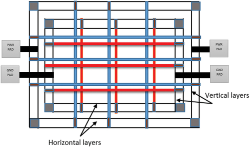
Power planning is a very important as well as crucial step in the floor planning step in IC design flow where power must be distributed to all parts of the design in the core to ensure equal supply. Distribution of power can be carried out manually by the design engineer or can be done using the Backend EDA tool. Distribution of power supply, i.e., VDD and GND, is done in three levels as See Figure 1. At first, there are rings which are formed around the core and the macro, second level is the stripes which carries VDD and GND around the chips and across the chips, and the third level is the stripes created around the core area to tap power from rings. The third level is the rails which connect VDD and GND to the standard cell. The drive to reduce the time to market and the design complexity has resulted in the early estimation of power at the specification level, which leads to proper estimation of the number of strips and pads and helps the floor plan engineer carry out accurate power planning. The use of ML in predicting power is a new paradigm. It needs previous knowledge of power dissipated by the circuits. We can train different ML models like SVM, K-Nearest Neighbor, RF, etc. Use of sophisticated tools will give accurate results at the cost of time. But our idea is to help the floor plan engineers come up with better power planning by estimating the power of the VLSI circuits using ML.

Figure 1. Power pads and Strips.

There are benchmark designs in the form of reference circuits presented at the International Symposium on Circuits and Systems (ISCAS). They offer RTL coding for a number of circuit types. The novelty and contribution lies in creating data set. We have taken all the benchmark circuits and performed pre-synthesis power calculations using Cadence EDA tool, which we refer to as data set 1, and also performed power calculations on benchmark circuits using cadence EDA tool targeting the 45 nm technology library (Referred to as Post-Synthesis) which we refer to as data set 2. Gate count, gate type, metal layer count and gate size, etc. Were all variables included in both data sets. The datasets were split into a training set and a test set. All of the ML models used were tested and trained using the collected data.

Literature Overview

In (Gupta and Najm 1999) the author proposed a modeling methodology which captures the dependency of the logic circuit power dissipation (both combinational and sequential) by signal switching statistics on its I/O. The estimate of the power consumption of the circuit for any given input and output was determined by the power model involving quadratic and cubic equations in four variables. Instead of power estimation, the author proposed a power reduction technique in (Shaktisinh, Popat, and Patel 2015), which used a compaction technique to save 33% of power consumed by reducing the number of test patterns used during verification. In (Kim, Limotyrakis, and Yang 2010) the author presented a multilevel design pipeline ADC approach to reduce the power dissipation. The power is minimized in the residue amplifier pipeline stage by jointly optimizing circuit-level type and voltage supply. The power is still minimized at the architecture level due to the non-linearity contribution, which is optimally distributed. In (Chaudhuri, Mishra, and Jha 2014) the author attempted to develop analytical models for leakage and delay estimation of FinFET logic gates. The author predicted the leakage current using analytical models, which used central composite rotatable design and response surface methodology. In (Bhanja and Ranganathan 2003) the authors proposed the switching activity estimation of very large-scale integration circuits using a Bayesian network. The author modeled the switching activity in the circuit using a logic-induced directed acyclic graph. In (Buyuksahin and Najm 2005), the author estimated the power at a high level of abstraction, i.e., during the specification phase. He estimated the power using the knowledge of total capacitance and the average switching activity of the design. It also uses Boolean network representation and correlated input streams. In (Hou, Zheng, and Wu 2006), the author calculated the power of circuits using neural networks. Even though simulation-based power estimation was the most accurate and time-consuming method, the author used benchmark (ISCAS89) circuits for estimating the power. In (Vellingiri and Jayabalan 2018) the author employed BPNN and ANFI systems to estimate the power of CMOS-based integrated circuits even without having knowledge of the structure and interconnection of the design. He also proposed that ANFIS had a very low RMSE and a high coefficient of determination. In (Kozhaya and Najm 2001) the author argued that the power was done only using the average signal probability of the inputs. The power estimation approach used blocks of consecutive vectors selected randomly from the user-supplied realistic set of input vectors, and a circuit was simulated for every block from an unknown state. In (Nasser, Prévotet, and Hélard 2018) the author compared the estimated power using the proposed neural network power models with the Xilinx power analyzer tool. He proved that the mean absolute error percentage was less than 8% when compared to the Xilinx power flow estimation of power. The author of (Nasser et al. 2020) conducted a survey on various power models and power estimation models for FPGAs and application-specific integrated circuits. He also classified the various approaches according to various metrics and gave an overview of RTL and transistor power modeling.

Background

Dissipation of Power

Dissipated total power See Figure 2. Can be categorized into two types, i.e., static power dissipation and dynamic power dissipation. Static dissipation means power dissipated by a transistor when it is not switching. It is mainly due to leakage current in standby mode See equation (1)(1) $I_{Sub}=A{e}^{\frac{q}{nkT}}\left(V_{GS}-V_{To}-\delta V_s+n{V}_{DS}\right)\left(1-e^{\frac{-qVds}{KT}}\right)$(1) . Leakage current happens when parasitic diodes form in the transistor’s substrate, when current flows in the sub threshold region, when current flows through the gates at higher voltages, or when tunneling currents flow.

(1) $I_{Sub}=A{e}^{\frac{q}{nkT}}\left(V_{GS}-V_{To}-\delta V_s+n{V}_{DS}\right)\left(1-e^{\frac{-qVds}{KT}}\right)$(1)

Figure 2. Sources of power dissipation and its comparison on different process technology.

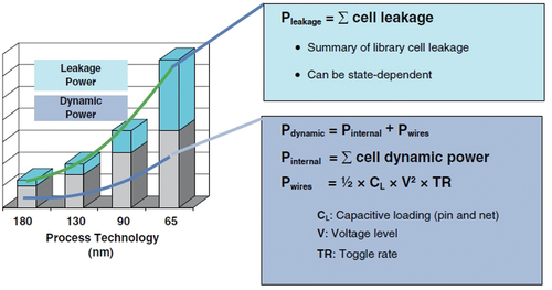
In equation 1, k denotes the Boltzmann constant, e is the electronic charge, T is the temperature, n is the swing coefficient, drain to source voltage is denoted by VDS, gate to source voltage is denoted by VGS, VT0 is the threshold voltage at zero bias, body effect coefficient is denoted by i, drain induced barrier lowering coefficient is denoted by s, and here, µ0 is the mobility at zero bias, Effective width and length are represented by W_eff, L_eff respectively and gate oxide capacitance per unit area is denoted by $C_{ox}$ See Eq. (2).

(2) $A={\mu }_o{C}_{ox}\frac{W_{eff}}{L_{eff}}{\left(\frac{kT}{q}\right)}^2{e}^{1.8}$(2)

Dynamic power dissipation shown in Figure 3. Occurs when the circuit is active, i.e., when the output load capacitance CL is charged and discharged due to the change in voltage on input net changes due to some stimulus applied. A change in the voltage of the input net may or may not lead to a change in the logic gate of the output. But in both cases, dynamic power will be dissipated See Eq. (3).

(3) $P_{Dynamic}=\frac{1}{2}f\left(V_{DD}^2{\sum }_i\left({\propto }_i{C}_{Li}\right)+V_{DD}{\sum }_i{\sum }_j\left({\propto }_{ij}{C}_{ij}{V}_{ij}\right)\right)$(3)

Figure 3. Dynamic Power dissipation.

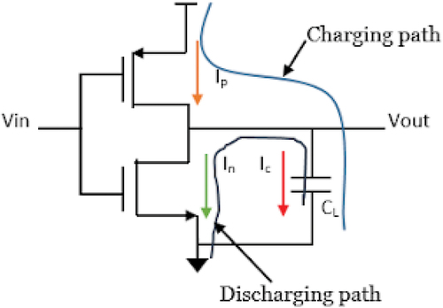
In the above equation, f is the clock frequency, α denotes activity factor, i represents the gate and j denotes the jth internal node in a gate. The voltage swing is represented by Vij. The load capacitance is represented by CLi and the jth internal node capacitance of gate I is represented by Cij (Girard 2002; Sharifi et al. 2005).

Machine Learning Algorithm/Models

SVM

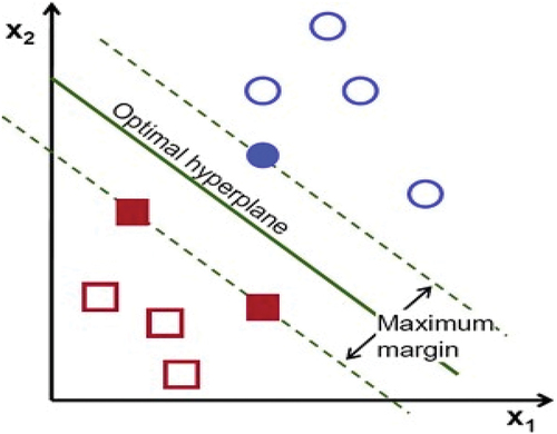
Support vector machines are a relatively new invention. Uses in remote sensing include pattern recognition and classification. Because of the rapid growth of data-intensive technologies and the associated delay in the development of analytical tools, ecologists and environmental scientists who use remote sensing for these purposes adopted SVMs (Gaye et al. 2021; Yu et al. 2016) earlier than their counterparts in other fields. However, the usage of SVMs (Hearst et al. 1998; Pradhan 2012) in a wide range of ecological fields has increased significantly in recent years. SVM is one of the finest nonlinear supervised machine learning models. Given a set of labeled training data, SVM will help us to find an optimal hyperplane which categorizes new examples. The hyperplane is a point; in one- and two-dimensional space, the hyperplane is a line, and in three-dimensional space, the hyperplane is a line that separates a space into two sections. Each class lies on either side. Let us first start with a two-dimensional, linear, separable case. The data are separated by a line, as shown in Figure 4.

Figure 4. Optimal hyperplane of SVM.

K-NN

A k-nearest neighbor is one of the critical and usually evident figures for activities, such as grouping; in this analysis, it has been used for missing data attribution (displacing missing characteristics with the closest feasible value). Usually, any variant may be used for attribution purposes; regardless of this, KNN is used in this review, as it is practical to do so. Figure 5 shows the representation of the KNN algorithm in graphical form.

Figure 5. Representation of KNN algorithm.

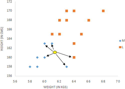
This is a simple and supervised machine learning algorithm. This group contains innovative examples reliant on convenience calculus, otherwise known as division calculus. This technique of results incorporates three partitions of actions: Eugène-Minkowski, a division of Euclide, and Midtown (Bajard, Didier, and Muller 1998).

1. The length of guidance is calculated by putting that element test and the name of the class preparing aside.

2. Those clients want to characterize k as “a collection of values for uncertain examples of k-number class marks, hence unmarked preparation of examples could be characterized dependent on similarity of class elements.

3. A survey based on the collection of casting happens on behalf of an unmarked group. Different strategies are nothing but heuristic systems of evaluation that work based on

Forest at Random

The Random Forest algorithm is another sophisticated machine learning technique used in regression and classification. The forest has trees, and a tree in the machine learning world means a decision tree. This is the reason we call it the Random Forest, see Figure 6 .

Figure 6. Decision Tree.

Random forest regression depends on the statistical method called bagging. (Biau 2012; Qiong Ren, Cheng, and Han 2017) Random forest regression uses less time to create a model on the hyper-parameter. It is also more flexible with all types of datasets. Because the random forest has a large number of decision trees, it reduces the variance on new data. The feature selection is applied over the random forest. It decreases the impurity tree.

(4) $Gini=1-{\sum }_{i=1}^C{\left(P_i\right)}^2$(4)

(5) $Entropy={\sum }_{i=1}^C-p_i\ast lo{g}_2\left(p_i\right)$(5)

This justification of the decision manic line has the rear of the support vector machine into datasets. This algorithm of the datasets can be divided into two classes and is depicted in see Figure 6. This incorporates the two stages: the observation of the benefits of an otherwise perfect manic line during an information gap, along with the restrictions determined by the mapping of objects (Huynh-Cam, Chen, and Le 2021).

Pre-Synthesis and Post-Synthesis

The term “Pre-synthesis” refers to a circuit designed without targeting any particular technology, and “Post-synthesis” refers to a circuit designed after targeting technology. In this work, we used the 45 nm technology library. During the pre-synthesis phase, power was predicted using the Cadence EDA tool for all the ISCAS 89 and ISCAS 99 benchmark circuits. See Tables 1 and 2 show a snippet view of the dataset of ISCAS benchmark circuits. Figure. 7 shows the implementation approach used in our paper.

Figure 7. Implementation approach.

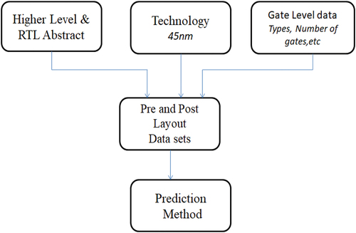
Table 1. Snippet View of Dataset (ISCAS 89).

Bench mark	IN	OUT	DFF	INV	GATE	AND	NAND	OR	NOR
S27	4	1	3	2	8	1	1	2	4
S208	10	1	8	38	66	21	15	14	16
S298	3	6	14	44	75	31	9	16	19
S344	9	11	15	59	101	44	18	9	30
S349	9	11	15	57	104	44	19	10	31
S382	3	6	21	59	99	11	30	24	34

Table 2. Snippet view of dataset (ISCAS 99).

Bench mark	IN	OUT	GATE	Nets	FF
b01	2	2	49	56	5
b02	1	1	28	33	4
b03	4	4	160	194	30
b04	11	8	737	814	66
b05	1	36	998	1033	34
b06	2	6	56	67	9
b07	1	8	441	491	49

The various features used for power prediction using ML models at the pre-synthesis phase are the number of inputs, gates like inverters, AND, OR, and for sequential circuits, flip-flops.

The data sets were separated as training data and testing data, and various ML models were applied for both the ISCAS 89 and 99 benchmark circuits, and a comparative study was conducted on the power prediction by the tool with the various ML algorithms. See Tables 3 and Table 4 for the power prediction values. PRE represents the power prediction by the tool at the pre-synthesis phase and POST represents the power prediction by the tool at the post-synthesis phase where a particular technology library is targeted See Tables 3 and Table 4. See Figures 8 and 9 above for the comparison of power predictions of ISCAS 89 benchmark circuits at the pre- and post-synthesis stage.

Figure 8. Power prediction comparison – Pre Synthesis- ISCAS 89.

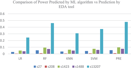
Figure 9. Power prediction Comparison – Post Synthesis- ISCAS 89.

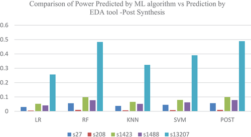
Table 3. Power predicted by ML algorithms and EDA tool at Pre-Synthesis Phase-ISCAS 89.

Bench mark	LR	RF	KNN	SVM	PRE
s27	0.028297	0.053313	0.035679	0.043061	0.055364
s208	0.004816	0.009074	0.006073	0.007329	0.009423
s1423	0.049549	0.093353	0.062475	0.075401	0.096944
s1488	0.038971	0.073424	0.049138	0.059304	0.076248
s13207	0.244288	0.460252	0.308015	0.371742	0.477954

Table 4. Power predicted by ML algorithms and EDA tool at post-synthesis phase-ISCAS 89.

Bench mark	LR	RF	KNN	SVM	POST
s27	0.029712	0.055979	0.037463	0.045214	0.056594
s208	0.005057	0.009528	0.006376	0.007695	0.009632
s1423	0.052026	0.098021	0.065598	0.079171	0.099098
s1488	0.04092	0.077095	0.051594	0.062269	0.077942
s13207	0.256502	0.483265	0.323416	0.390329	0.488575

The various features used for power prediction using ML models at the post-synthesis phase are the number of inputs, gates like inverters, AND, OR, flip-flops, the number of metal layers used, the RC value of gates and capacitance. Figures 10 and Figure 11 compare the power predictions of ISCAS 89 benchmark circuits at the pre- and post-synthesis stages. Table 5 and 6shows the power predicted by ML algorithms and EDA tool at pre-synthesis phase and psot-synthesis phase

Figure 10. Power prediction Comparison – Pre Synthesis- ISCAS 99.

Figure 11. Power prediction Comparison – Post Synthesis- ISCAS 99.

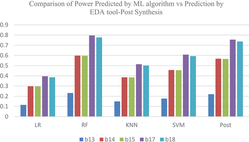
Table 5. Power predicted by ML algorithms and EDA tool at pre-synthesis phase-ISCAS 99.

Bench Mark	LR	RF	KNN	SVM	PRE
b13	0.112782	0.212487	0.142203	0.168355	0.22066
b14	0.291509	0.54922	0.367555	0.435151	0.570343
b15	0.290515	0.547347	0.366301	0.433667	0.568399
b17	0.387677	0.730406	0.48881	0.578706	0.758499
b18	0.378317	0.712771	0.477008	0.564734	0.740185

Table 6. Power predicted by ML algorithms and EDA tool at post-synthesis phase-ISCAS 99.

Bench Mark	LR	RF	KNN	SVM	Post
b13	0.115037	0.231447	0.149313	0.176773	0.219679
b14	0.297339	0.598227	0.385932	0.456908	0.567809
b15	0.296325	0.596187	0.384616	0.455351	0.565872
b17	0.395431	0.795581	0.513251	0.607642	0.755128
b18	0.385883	0.776372	0.500859	0.592971	0.736896

Comparative Studies of RF, KNN, SVM, and LR

Root Mean Square Error (RMSE) and Coefficient of Determination (R) are two statistical approaches that may be used to evaluate the GB networks’ performance; see Eq. (6) and Eq. (7).

(6) $RMSE=\sqrt{\frac{\sum _{i=1}^N{\left(Y_i^o-Y_i^c\right)}^2}{N}}$(6)

(7) $R={\displaystyle \sum _{i=1}^N\left(Y_i{}^o-Y^o\right)}\left(Y_i{}^c-Y^c\right){\displaystyle \sum _{i=1}^N{\left(Y_i{}^o-Y^o\right)}^2}\sum Ni=1{\left(Y_i{}^c-Y^c\right)}^2$(7)

Where $Y^o$ stands for the median of the observed value and $Y_i^o$ stands for the actual value that was measured. Computed value $Y_i^c$,calculated value$Y^c$. The root-mean-squared error (RMSE) measures how far actual values deviate from predictions. Precision or accuracy of models may be quantified by the root mean square error (RMSE). RF and models will have small RMSE values, if not RMSE values of zero See Tables 7 and 8.

Table 7. Evaluation of KNN, SVM and LR statistical methods.

Parameter	KNN	LR	RF	SVM
RMSE	0.0004398	0.000136	0.000106	0.000112
R	0.85765	0.89979	0.99879	0.98658

Table 8. Validation of the suggested random forest algorithm’s accuracy.

Selected benchmark circuit(ISCAS 99)	Actual output	Random Forest	Precision
b13	0.22066	0.212487	96.29611
b14	0.570343	0.54922	96.29644
b15	0.568399	0.547347	96.29626
b17	0.758499	0.730406	96.29624
b18	0.740185	0.712771	96.29633

Conclusions and Results

Even though there were a lot of power estimation techniques using different tools and technology, there was not a methodology for calculating the power of VLSI circuits at specification level and without having knowledge about the circuits. Predicting power with ML models is less expensive than using EDA tools. The novelty in our work is that we have calculated for both pre-synthesis and post-synthesis, which includes transistor physical sizes and interconnection details. Machine learning algorithms used were linear regression, Random Forest, KNN, SVM. The Random Forest model predicted the power, which was very close to the power predicted by the EDA tool. If you consider the B14 benchmark circuit, the power predicted by RF was 0.59 mW, the power predicted by the EDA tool was 0.567 mW, and the error percentage was 4. The error percentage for RF varied between 1% and 5%, whereas it varied more than 5% in all other models. This methodology can be enhanced to predict power for SoC and FPGA-based circuits.

Disclosure statement

The Author does not have any conflict of interest in submitting the paper to this journal.

References

- Bajard, J. C., L. S. Didier, and J. M. Muller. 1998. A new Euclidean division algorithm for residue number systems. Journal of VLSI Signal Processing Systems for Signal, Image, and Video Technology 19 (2):167–3669. doi:10.1023/A:1008065819322.
- Bhanja, S., and N. Ranganathan. 2003. Switching activity estimation of VLSI circuits using Bayesian networks. IEEE Transactions on Very Large Scale Integration (VLSI) Systems 11 (4):558–67. doi:10.1109/TVLSI.2003.816144.
- Biau, G. 2012. Analysis of a random forests model. Journal of Machine Learning Research 13 (1):1063–95.
- Buyuksahin, K. M., and F. N. Najm. 2005. Early power estimation for VLSI circuits. IEEE Transactions on Computer-Aided Design of Integrated Circuits and Systems 24 (7):1076–88. doi:10.1109/TCAD.2005.850904.
- Chaudhuri, S. M., P. Mishra, and N. K. Jha. 2014. Accurate leakage/delay estimation for FinFET standard cells under PVT variations using the response surface methodology. ACM Journal on Emerging Technologies in Computing Systems (JETC) 11 (2):1–20. doi:10.1145/2665066.
- Gaye, B., D. Zhang, A. Wulamu, and S.-B. Tsai. 2021. Improvement of support vector machine algorithm in big data background. Mathematical Problems in Engineering 2021: 1–9. doi:10.1155/2021/5594899.
- Girard, P. 2002. Survey of low-power testing of VLSI circuits. IEEE Design & Test of Computers 19 (3):82–92. doi:10.1109/MDT.2002.1003802.
- Gupta, S., and F. N. Najm. (1999, March). Analytical model for high level power modeling of combinational and sequential circuits. In Proceedings IEEE Alessandro Volta Memorial Workshop on Low-Power Design (pp. 164–72). IEEE. doi:10.1109/LPD.1999.750417.
- Hearst, M. A., S. T. Dumais, E. Osuna, J. Platt, and B. Scholkopf. 1998. Support vector machines. IEEE Intelligent Systems and Their Applications 13 (4):18–28. doi:10.1109/5254.708428.
- Hou, L., L. Zheng, and W. Wu. (2006, October). Neural network based VLSI power estimation. In 2006 8th International Conference on Solid-State and Integrated Circuit Technology Proceedings (pp. 1919–21). IEEE. doi:10.1109/ICSICT.2006.306506.
- Huynh-Cam, T. T., L. S. Chen, and H. Le. 2021. Using decision trees and random forest algorithms to predict and determine factors contributing to first-year university students’ learning performance. Algorithms 14 (11):318. doi:10.3390/a14110318.
- Kim, J., S. Limotyrakis, and C. K. K. Yang. 2010. Multilevel power optimization of pipelined A/D converters. IEEE Transactions on Very Large Scale Integration (VLSI) Systems 19 (5):832–45. doi:10.1109/TVLSI.2010.2041077.
- Kozhaya, J. N., and F. N. Najm. 2001. Power estimation for large sequential circuits. IEEE transactions on very large scale integration (VLSI) systems. 9 (2): 400–07. doi:10.1109/92.924063.
- Nasser, Y., J. Lorandel, J. C. Prévotet, and M. Hélard. 2020. RTL to transistor level power modeling and estimation techniques for FPGA and ASIC: A survey. IEEE Transactions on Computer-Aided Design of Integrated Circuits and Systems 40 (3):479–93. doi:10.1109/TCAD.2020.3003276.
- Nasser, Y., J. C. Prévotet, and M. Hélard. (2018, May). Power modeling on FPGA: A neural model for RT-level power estimation. In Proceedings of the 15th ACM International Conference on Computing Frontiers (pp. 309–13). doi:10.1145/3203217.3204462.
- Pradhan, A. 2012. Support vector machine-a survey. International Journal of Emerging Technology and Advanced Engineering 2 (8):82–85.
- Ren, Q., H. Cheng, and H. Han. (2017, March). Research on machine learning framework based on random forest algorithm. In AIP conference proceedings (Vol. 1820, No. 1, p. 080020). AIP Publishing LLC. doi:10.1063/1.4977376.
- Shaktisinh, J., J. Popat, and R. Patel. 2015, December. Power reduction techniques used in testing of VLSI circuits. In 2015 Annual IEEE India Conference (INDICON) (pp. 1–4). IEEE. doi: 10.1109/INDICON.2015.7443367.
- Sharifi, S., J. Jaffari, M. Hosseinabady, A. Afzali-Kusha, and Z. Navabi. 2005, March. Simultaneous reduction of dynamic and static power in scan structures. In Design, Automation and Test in Europe, 846–51. IEEE. doi:10.1109/DATE.2005.270.
- Vellingiri, G., and R. Jayabalan. 2018. Adaptive neuro fuzzy inference system-based power estimation method for CMOS VLSI circuits. International Journal of Electronics 105 (3):398–411. doi:10.1080/00207217.2017.1357763.
- Yu, J. S., A. Y. Xue, E. E. Redei, and N. Bagheri. 2016. A support vector machine model provides an accurate transcript-level-based diagnostic for major depressive disorder. Translational Psychiatry 6 (10):e931. doi:10.1038/tp.2016.198.