A Multi-Model Prediction Method for Coal Mine Gas Concentration with Hierarchical Structure

ABSTRACT

The low concentration of gas in the gas blending process is influenced by a number of factors and is characterized by some time variation and non-linearity. Therefore, the gas concentration needs to be predicted. This paper proposes a multi-model forecasting method with a hierarchical structure. First, because the measured gas concentration time-series data contain a lot of noise, the time-series data are decomposed into several independent eigenmode functions by using empirical mode decomposition, adaptively denoising by low-pass filtering, and then using phase space reconstruction technology to obtain a new time-series sample. Then, the training samples are grouped by conditional fuzzy clustering to determine the number of sub-modules. Finally, the maximum membership method is used to select sub-models and sub-sub-models, and then a multi-model time-series prediction model is established. The model can not only select different sub-models to process data in different regions but also can process each data jointly by multiple sub-models in different sub-models. Experiments were carried out on low-concentration measured data extracted from mines. The experimental results show that the proposed prediction model can capture the nonlinear characteristics of gas concentration time series and is superior to other existing prediction models in accuracy.

Introduction

China has very rich coal resources, and the consumption and output of coal are very high (Niu et al. 2020). As the coal seam is mined from shallow to deep, the amount of gas released by the coal seam increases significantly. However, the concentration of the extracted gas is low and the fluctuation is large (Qiao et al. 2011; Wang et al. 2021), so it cannot be directly sent to the generator set for power generation. In addition, the main component of gas, CH4, is a greenhouse gas. If gas is directly released into the air, it will have a greenhouse effect that is about 21 times greater than that of carbon dioxide (Nisbet et al. 2019). This leads to serious environmental and economic concerns (Sohani et al. 2022). The use of gas blending technology maximizes the use of the gas extracted from the mine. The gas extracted from the mine is mixed with a certain proportion of gas, and the gas whose concentration meets the requirements of gas power generation is sent to the generator set for power generation (Zhang 2019). It can not only alleviate the shortage of power supply in coal mining areas but also generate huge ecological and economic benefits, and reduce the threat of coal mine gas disasters (Li et al. 2021).

At present, the law of coal seam gas gushing is still unclear, and it is difficult to determine the only concentration value of gas extracted from mines. When the gas blending technology is used to mix the gas extracted from the mine with the gas with a certain concentration, there are certain pure lag and nonlinear links, and the tracking performance and anti-interference performance of the traditional PID control are poor (Jin and Son 2019). The prediction result of mine gas concentration directly affects the control precision and control effect of the gas blending system. Therefore, a multi-model prediction method with hierarchical structure is proposed.

The gas concentration in the actual mine is a complex nonlinear dynamic system affected by many factors such as natural factors and mining technology (Song et al. 2019). Therefore, traditional prediction methods such as gas geological unit method and index method cannot guarantee the accuracy of gas prediction. In recent years, the prediction of gas concentration mainly uses neural networks (Du et al. 2019; Yin, Li, and LI 2013), chaos theory prediction (Li, Han, and Wang 2012), data fusion (Guo and Li 2018) and differential gray model (Zeng and Li 2021) and radial basis function forecasting model (Zhou et al. 2017) to judge gas outburst by predicting the amount of gas gushing out of mines. Extensive research has been conducted in the area of mine gas concentration forecasting. Liu, Zhao, and Hao (2015) proposed a prediction method combining Genetic Algorithm (GA) with Backpropagation (BP) neural network that improves the accuracy and reliability of gas concentration prediction, but has certain limitations due to the small data sample, and it is difficult to adapt to complex and variable gas concentration sequences. Zhang et al. (2019) proposed a gas concentration prediction method based on LSTM multidimensional time series. However, LSTM has many parameters and a complicated structure, which is prone to overfitting problems. Jia and Deng (2012) proposed a combined forecasting model for mine gas concentrations based on a pan-average calculation. In addition, Jia et al. (2020) proposed a gas concentration prediction method based on Gated Recurrent Units (GRUs), but a GRU only considers the forward information in a sequence and does not consider the reverse information. In most cases, considering the reverse information can improve the forecasting accuracy of the model. The above prediction models are all single-model prediction models, and the data on the concentration of the extracted gas come from different areas in the mine. These data from different areas have different disturbance amplitudes and object characteristics. If a single-model prediction model is used, it will often lead to defects such as long learning time, poor accuracy and extrapolation ability. In addition, in the face of complex nonlinear dynamic systems, the single model also has the problem of forgetfulness, which makes its adaptive ability and robustness weak (Bo, Qiao, and Yang 2011).

Hybrid models are being proposed to overcome the limitations of single models and increase the forecasting performance. Karasu and Altan (2022) proposed a deep learning model that uses an optimization algorithm based on a logical chaos graph to select its features, including technical indicators such as LSTM neural network, trend, volatility, and momentum, and the CHGSO algorithm to overcome these difficulties and forecast crude oil prices with high accuracy. Karasu et al. (2020) also proposes a novel prediction model based on RBFSVR, which employs a wrapper-based feature selection method to handle such non-stationary and nonlinear factors using a meta-heuristic-based multi-objective optimization technique. Altan, Karasu, and Zio (2021) proposes a new hybrid WSF model based on Long Short Term Memory (LSTM) network and Grey Wolf Optimizer (GWO) decomposition method. In the preprocessing stage, the missing data are filled by the weighted moving average (WMA) method, the WS time series (WSTS) data are smoothed by WMA filtering, and the smoothed data are normalized by Z-score as the model input. Subsequently, combining LSTM and decomposition method, a hybrid WSF model is established, and the Intrinsic Mode Function (IMF) of the estimated output is optimized by the Grey Wolf Optimizer (GWO).

The multi-model prediction model based on decomposition and combination rules can also overcome the limitations of a single model to a certain extent and improve the prediction performance (Perendeci et al. 2008), and the multi-model prediction model has been successfully applied to continuous stir tank reactors (Pipino, Cappelletti, and Adam 2021) and the medical field (Prakash et al. 2021). At the same time, A multi-model prediction model with a hierarchical structure was successfully used for temperature control (Pang et al. 2012). The measured gas concentration data in mines generally contains a lot of noise. If the data containing noise is directly used for prediction, the prediction accuracy will often deteriorate. Soltani (2002) proposes a prediction method of wavelet decomposition and reconstruction for noisy time-series data, but the wavelet analysis of this method needs to determine the basis function and decomposition scale in advance, and after selecting the basis wave, all historical data must be recalculated. Therefore, the method is less flexible and adaptive.

The main contributions of this paper are summarized as follows:

1. Modal decomposition is used to decompose the gas concentration data containing noise into multiple eigenmode functions, and the first three IMFs are selected for prediction. Since the process is based on the adaptive decomposition of the gas concentration data itself, there is no need to select a basis function. Then, the decomposed small-scale eigenmode function is adaptively denoised by using a low-pass filter, and the phase space reconstruction of the denoised gas concentration sequence data is carried out.

2. The training samples are grouped by conditional fuzzy clustering to determine the number of sub-modules. The maximum membership method is used to select sub-models and sub-sub-models. In order to further optimize the multi-model prediction model, the fuzzy membership threshold is set. It is used to further eliminate the sub-sub-models that are not suitable for learning the input samples in the selected sub-sub-models.

3. A multi-model prediction model with a hierarchical structure is adopted, which can not only select different sub-models to process data in different regions but also each data is co-processed by multiple sub-sub-models in different sub-models. Thus, the final output of the multi-model prediction model is an integration of the sub-model and sub-sub-model outputs of the latter two levels of neurons. This learning approach is also clearly different from the traditional multi-model prediction measurement model.

The method in this paper is used to predict the gas concentration in the actual mine, experimental results show that the prediction accuracy is higher than that of the single model prediction method currently applied.

The remainder of this paper is organized as follows. Section 2 presents the construction process of the gas concentration time-series prediction model, including the empirical mode decomposition to remove the noise of the gas data and the reconstruction of the gas concentration time series. Section 3 presents the structure of the multi-model prediction model, as well as the selection of sub-models and sub-sub-models, and the network learning algorithm. Section 4 presents the simulation process and experimental results. Section 5 discusses the results of the experiment and analyzes the causes of the results. Section 6 introduces the conclusion, and uses the method proposed in this paper to predict the measured mine gas concentration time-series data, and obtains a satisfactory result, which provides decision support for subsequent gas blending control.

Construction of Gas Concentration Time-Series Prediction Model

Empirical Mode Decomposition Denoising

The measured mine gas concentration data usually contain a large amount of noise. The simulation finds that the prediction accuracy is still greatly affected by noise when the multi-model prediction model proposed in this paper directly uses the original gas concentration data. To solve this practical problem, this paper uses EMD to denoise the original gas concentration data before prediction. The traditional EMD denoising method will treat the small-scale IMF as noise to eliminate, and this method simultaneously removes useful information. Considering that when the noise level in the gas concentration data is high, the standard deviation between adjacent signals will be relatively large, so the standard deviation can be used as the basis for judging the noise level, and only use a low-pass filter to denoise the gas concentration data with high noise.

The denoising process is described in detail as follows:

Step 1 Find all the local extreme points of the signal $x(t)$, and use the interpolation method to form the upper and lower envelopes of the signal. Calculate the average value $m_1$ of the two envelopes, denote as the difference between $x(t)$ and $m_1$, and repeat the above process until $h_1$ satisfies the definition of IMF. Let the result of the $p$-th step be $h_{1p}=h_1(p-1)-m_{1p}$, denote $h_{1p}=c_1$, then $c_1$ is an IMF decomposed from the original data.

Step 2 Take $r_1=x(t)-c_1$ as the decomposition data, repeat the above process until the residual quantity is monotonic or constant, and finally decompose the signal into a residual component $r_n$ and $n$ IMFs, namely:

(1) $x(t)=\sum _{i=0}^n(c_i+r_n)$(1)

Step 3 Use the first $p$ IMF components to denoise, and use an adaptive threshold $T_i=(i-1{)}^2{o_i}^{\prime }/n^2$, $1\le i\le p$, where ${o_i}^{\prime }$ represents the standard deviation of the $i$th scale signal.

Step 4 Calculate the standard deviation $o_{ij}$ of the $i$th signal and its neighboring signals. If $o_{ij}>T_i$, a low-pass filter is used to denoise the signal.

The denoised IMF components and the remaining $n-p$ components are reconstructed in phase space to obtain the denoised gas concentration time-series data.

Gas Concentration Time-Series Reconstruction

The time series of gas concentration after denoising is $\{x(t)=|t=1,2,\dots ,N\}$, Taking the time delay $\tau$ and the embedding dimension $m$, the reconstructed phase space is:

(2) $X=\{x(i)=|i=1,2,\dots ,M\}=[x(1),x(2),\dots ,x(M)]$(2)

where $x(i)$ is the point in the phase space; $M=N+(m-1)\tau$ is the number of phase points, $m$ is the dimension of the embedded phase space, and $\tau$ is the time delay.

Define the correlation integral of the gas concentration series as:

(3) $C(m,N,r,t)=\frac{2}{M(M-1)}\sum _{1\le i<j<M}\phi (r-d_{ij}),r>0$(3)

where $d_{ij}=||x(i)-x(j)|{|}_{(\mathrm{\infty })}$; $\phi (x$) is the impulse function, when $x\ge 0$, $\phi (x)=1$, when $x<0$,$\phi (x)=0$; $C(m,N,r,t)$ is a cumulative distribution function, which represents the probability that the phase point $x(j)$ in the phase space falls into the sphere with the phase point $x(i)$ as the center and the radius is less than $r$.

The test statistic is defined as:

(4) $S(m,N,r,t)=C(m,N,r,t)-C^m(1,N,r,t)$(4)

Select the largest and smallest two radii $r$, and define the difference as:

(5) $\mathrm{\Delta }S(m,t)=max\{S(m,N,r_j,t)\}-min\{S(m,N,r_j,t)\}$(5)

where $\mathrm{\Delta }S(m,t)$ is the maximum deviation of $S(m,N,r,t)$ for all radii $r$.

Reasonable estimates of $M$, $n$ and $r$ can be obtained based on the BDS statistical conclusions and combined with experiments (Kim, Eykholt, and Salas 1999). This paper selects = 2,3,4,5. $r_j=j\sigma /2$, $\sigma =std(x)$. According to the above values, it can be calculated:

(6) $\bar{S}(t)=\frac{1}{16}\sum _{m=2}^5\sum _{j=1}^{4}S(m,r_j,t)$(6)

(7) $\mathrm{\Delta }\bar{S}(t)=\frac{1}{4}\sum _{m=2}^5\mathrm{\Delta }S(m,t)$(7)

The $\tau$ corresponding to the first local minimum of $\mathrm{\Delta }S(t)(0\le t\le 200)$ is the optimal time delay $\tau$.

Define another indicator:

(8) $S_{cor}(t)=\mathrm{\Delta }\bar{S}(t)+|\bar{S}(t)|$(8)

The value of $t$ corresponding to the global minimum value of $S_{cor}(t)(0\le t\le 200)$ is time window s${\tau }_w$. From ${\tau }_w=(m-1)\tau$, $m=1+{\tau }_w/\tau$ can be obtained.

Multi-Model Predictive Models

Multi-Model Prediction Model Structure

The multi-model prediction model proposed in this paper is shown in Figure 1

Figure 1. The architecture of the multi-model.

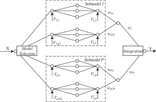
Predictive models use a hierarchical approach to deal data. First, the selection of different sub-models and sub-sub-models in the multi-model prediction model for different input samples via the model selection layer. The multi-model prediction model consists of $P$ sub-models, and each sub-model includes $C_i$ sub-sub-models of varying numbers. Each specific sub-sub-model is a feed-forward neural network with a relatively simple structure, and its main task is to learn the input samples assigned by the model selection layer.

Without loss of generality, let the network structure of the $C_i$th sub-sub-model in the $P$-th sub-model is $n-m-1$($n$ input nodes, $m$ hidden nodes, $1$ output node), then the output of this sub-sub-model is:

(9) $y_{c_i}(k)=\sum _{j=1}^m{w}_j(k)f\left(\sum _{i=1}^n{v}_{ji}(k)x_i(k)\right)$(9)

where $w_j$ is the connection weight between the $j$th hidden node in the hidden layer of the sub-sub-model and the output node; $v_{ji}$ is the connection weight between the $i$th input node in the input layer and the $j$th hidden node in the hidden layer in the sub-sub-model;the function $f()$ is the activation function of the hidden node.

It should be noted that the activation functions of hidden nodes in different sub-sub-models of the multi-model prediction model in this paper can be different, which is obviously different from the traditional multi-model prediction model.

The final output of the multi-model prediction model is obtained by integrating the outputs of the sub-model and the sub-sub-model respectively by the latter two levels of neurons, that is, during learning, for a certain input sample, a certain selection strategy is used to select from different sub-models. A suitable sub-sub-model is learned on this sample. This learning method is also significantly different from traditional multi-model prediction models.

The multi-model predictive model learning process mainly includes three parts: sub-model and sub-sub-model partitioning, model selection and model output integration.

Division of Sub-Models

The use of clustering method to divide sub-models is a common method for multi-model structure design (Park, Pedrycz, and Oh 2009). Conditional fuzzy clustering can use the target value as a guide for sample clustering, so its clustering results are more objective (Pedrycz 1998). This paper will use the conditional fuzzy clustering method to realize the division of sub-models.

Given a multi-model training sample set $\{(x_k,y_k),k=1,2,\dots ,N\}$, First perform subtractive clustering on $y_k$, Let the result of $y_k$ subtractive clustering be $\{V_{y,1},\dots ,V_{y,p}\}$, That is $y_k$ has a total of $P$ cluster centers. According to formula (9), the target set $y_k$ is constructed into $P$ fuzzy sets. According to this $P$ fuzzy sets, the entire prediction model can be divided into $P$ sub-models.

(10) $f_{ik}=\left\{\begin{array}{c}exp\left(\frac{-\parallel y_k-V_{y,i}{\parallel }^2}{{\left(\frac{V_{y,i}-V_{y,i-1}}{2}\right)}^2}\right),y_k\le V_{y,i}\\ exp\left(\frac{-\parallel y_k-V_{y,i}{\parallel }^2}{{\left(\frac{V_{y,i+1}-V_{y,i}}{2}\right)}^2}\right),y_k>V_{y,i}\end{array}\right.$(10)

where $f_{ik}$ is the fuzzy membership degree that the sample $y_k$ belongs to the $i$th fuzzy set.

For each fuzzy set of the target set $y_k$, the input $x_k$ is subjected to conditional fuzzy clustering according to Equation 11(11) $V_{ij}=\sum _{k=1}^N(u_{ijk}{)}^a{x}_k/(u_{ijk}{)}^a$(11) and (Equation 12(12) $u_{ijk}=f_{ik}/\sum _m^{C_i}{\left(\frac{||x_k-V_{ij}||}{||x_k-V_{im}||}\right)}^{\frac{2}{b-1}}$(12) ).

(11) $V_{ij}=\sum _{k=1}^N(u_{ijk}{)}^a{x}_k/(u_{ijk}{)}^a$(11)

(12) $u_{ijk}=f_{ik}/\sum _m^{C_i}{\left(\frac{||x_k-V_{ij}||}{||x_k-V_{im}||}\right)}^{\frac{2}{b-1}}$(12)

where $V_{ij}$ is the cluster center of the $j$th training sample fuzzy set corresponding to the $i$th fuzzy set of $y_k$, where $i=1,\dots ,P,j=1,\dots ,C_i$, $C_i$ indicates the number of fuzzy clusters of training samples corresponding to the $i$th fuzzy set of $y_k$.constants a and b, and generally take the value 2.

$\left[u_{ijk}\right]\in R^{C_i\times N}$ represents the segmentation matrix of the fuzzy clustering of the training samples corresponding to the $i$th target fuzzy set, which satisfies:

(13) $\sum _{j=1}^{C_i}{u}_{ijk}=f_{ik},u_{ijk}\in [0,1]$(13)

Using the above method, the training sample set of the multi-model prediction model can be divided into $C_T$ sample subsets:

(14) $C_T=\sum _{i=1}^P{C}_i$(14)

In the multi-model prediction model, each of the divided training sample subsets corresponds to a sub-sub-model, and there are $P$ sub-models in the entire multi-model prediction model ($M_i$ represents the $i$th sub-model, $i$ = 1, …, $P$), the $P$ sub-models also include $C_T$ sub-sub-models (represented by $M_{ij}$, $j$ = 1, …, $C_T$) to learn the corresponding sample set.

Sub-Model and Sub-Sub-Model Selection

According to the above method of dividing the training sample set, there must be a certain affiliation between the training sample set and the sub-model. According to the theory that similar inputs produce similar outputs, if the distance between the input sample $x_k$ and the cluster center $V_{ij}$ is relatively close, the possibility that $x_k$ belongs to the sub-sub-model $M_{ij}$ is relatively high. The relative distance measure can be used to measure the degree to which $x_k$ belongs to $M_{ij}$:

(15) $J_i=\sum _j^{C_i}{w}_{ij}{d}_{ij}$(15)

In the formula, ${\sum }_{j=1}^{C_i}{w}_{ij}=1$,$w_{ij}\in [0,1]$; $d_{ij}=||x_k-V_{ij}||/d{a}_{ij}$ is the relative distance measure between the input sample $x_k$ and the sub-sub-model $M_{ij}$, $d{a}_{ij}=\frac{1}{N_{ij}}{\sum }_{m=1}^{N_{ij}}||x_m-V_{ij}||$ is the average distance between all training samples in the sub-sub-model $M_{ij}$, $N_{ij}$ is the total number of training samples of the sub-sub-model $M_{ij}$; $w_{ij}$ is the membership degree of the input sample $x_k$ to the sub-sub-model $M_{ij}$.

To minimize the performance index $J_i$, the Lagrange multiplier method is used calculate $w_{ij}$:

(16) $w_{ij}=\left\{\begin{array}{c}1,when{d}_{ij}=0\\ \frac{d_{ij}^{-1}}{{\sum }_{j=1}^{C_i}{d}_{ij}^{-1}},otherwise\end{array}\right.$(16)

It can be seen from Equation 14(14) $C_T=\sum _{i=1}^P{C}_i$(14) that the larger the $d_{ij}$, the smaller the $w_{ij}$, which means that the probability of $x_k$ belonging to $M_{ij}$ is smaller; on the contrary, the probability of $x_k$ belonging to $M_{ij}$ is greater.

In this paper, the maximum membership degree method is used to select the sub-sub-model suitable for learning the input sample $x_k$, and the selected sub-sub-model is set as $M_{is}$. If $w_{is}$ = 1, $w_{ijj\ne s}$ = 0, the above selection method will select a sub-sub-model in each sub-model to learn the input sample $x_k$. At this time, the output of each sub-model is essentially the output of the selected sub-sub-model $M_{is}$.

In order to further optimize the multi-model prediction model, this paper adopts a secondary optimization strategy, that is, the sub-sub-models that are not suitable for learning the input sample $x_k$ are further eliminated from the selected sub-sub-models. The removal method is as follows:

For the first selected sub-sub-model to build the performance indicator function, let

(17) $J=\sum _i^P{w}_i{d}_i$(17)

where ${\sum }_{i=1}^P{w}_{ij}=1$,$w_{ij}\in [0,1]$; $d_i=||x_k-V_i||/d{a}_i$ is the relative distance measure between the input sample $x_k$ and the sub-sub-model $M_{is}$, $d{a}_i=\frac{1}{N_i}{\sum }_{j=1}^{N_i}||x_j-V_i||$ is the average distance between all training samples in the sub-sub-model $M_{is}$.

$N_{ij}$ is the number of training samples of the sub-sub-model $M_{is}$;$V_i$ is the cluster center of the training samples of $M_{is}$,$w_i$is the fuzzy membership degree of the input sample $x_k$ belonging to the sub-sub-model $M_{ij}$.

To minimize the performance index $J_i$, the Lagrange multiplier method can be used calculate $w_i$:

(18) $w_{ij}=\left\{\begin{array}{c}1,when{d}_i=0\\ \frac{d_i^{-1}}{{\sum }_{i=1}^P{d}_i^{-1}},otherwise\end{array}\right.$(18)

Since the selection of sub-models and sub-sub-models adopts the maximum membership degree method. Thus, each training sample in the training sample set is affiliated to each sub-model with a certain fuzzy affiliation. Due to the overlapping characteristics of training samples, a fuzzy membership threshold $K$ can be set.

Only sub-sub-models satisfying $w_i>K$ can be selected to learn the input sample $x_k$.

Integration the Output of Sub-Models

Suppose that the training sample is $x_k$, let $w=\{w_1,\dots ,w_p\}$, if $w_i<K$, set $w_i=0$, normalize $w$. Then, the final output of the multi-model prediction model is:

(19) $Y=\sum _{i=1}^C{w}_i{y}_i$(19)

where $w_i$ is the normalized weight of $M_{is}$; $y_i$ is the output of $M_{is}$ to $x_k$.

Analysis of Model Complexity and Parameter Uncertainty

The parameters to be determined in this paper are the number of sub-models P, the number of sub-sub-models C and the fuzzy subordination threshold K. The number of sub-models and the number of sub-sub-models are clustered using a fuzzy conditional clustering method, and the result of the clustering is the number of sub-models and sub-sub-models. The fuzzy subordination threshold is generally in the range of 0.05–0.2. If the value of K is too large, the training data of each sub-model will overlap and reduce the performance of the method; if the value of K is too small, each sub-model will be relatively independent and the boundary data will not be processed effectively, which will also reduce the performance of the method.

Regarding complexity, the multi-model approach with a hierarchical structure divides the training samples by clustering, and the training sample data is divided into sub-sub-models under multiple sub-models for processing, with each model processing only a specific amount of data (any learning sample can only activate a part of that network region), so for a complex task, the approach works better than one model processing the entire training sample, and this paper uses an experimental. The complexity of the proposed method is measured in an experimental manner. This is further explained in the experimental section of Section 4.

Experiment

In order to verify the validity of the proposed multi-model for predicting the gas concentration in the mine, the underground gas concentration $\{x(t)|t=1,2,\dots ,500\}$ of a coal mine with a sampling interval of 10 min was collected for experimental analysis.

The graph of the time-series data of gas concentration with noise is shown in Figure 2

Figure 2. The raw time-series data of gas concentration.

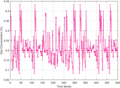
As can be seen from Figure 2, the data fluctuates greatly randomly.

The corresponding relationship between the amplitude and time of EMD decomposition of the gas concentration time-series data with noise is shown in Figure 3.

Figure 3. The EMD result of the raw data.

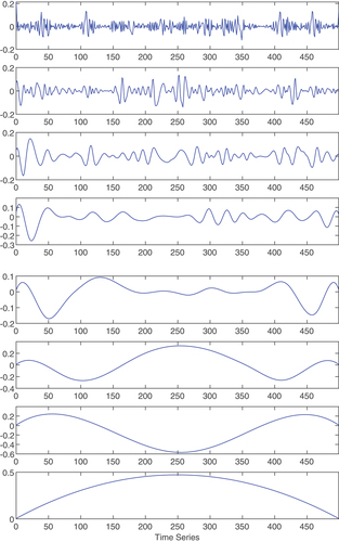
It can be seen from Figure 3 that seven IMFs and a residual amount are obtained by EMD decomposition of the data. In this paper, low-pass filtering is used to denoise the first three IMFs after EMD decomposition.

The correlation integration method is used to reconstruct the phase space of the denoised time-series data. The embedded dimension of the time series is calculated as $m$ = 5, and the corresponding time delay $\tau$ = 2; therefore, the input of the neural network is $[x(t)x(t-2)x(t-4)x(t-6)x(t-8)]$. Combining the practical needs of gas blending control systems, this paper predicts the change of gas concentration after 20 min, the output of the neural network is $x(t+2)$. The denoised and reconstructed gas time-series graph is shown in Figure 4.

Figure 4. The time-series data after denoising.

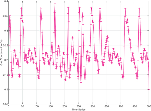
Comparing Figures 3 and 4, it can be seen that the denoising method in this paper can better retain the useful information in the gas concentration time series while denoising, and the denoising effect is ideal.

The multi-model prediction model proposed in this paper is used to predict the gas concentration time series reconstructed by denoising, and the data after phase space reconstruction is 489 groups. During the experiment, the first 300 groups were selected as training data, and the last 189 groups were selected as test data. During the experiment, the parameters of the multi-model prediction model are:$P=4,C=\{3,4,4,3\}$ is the number of sub-sub-models in each sub-model, $K=0.1$, the number of hidden layer neurons in each sub-sub-model is 8, and the learning algorithm of each sub-sub-model adopts the gradient descent method. It is compared with the prediction effect of the single-model prediction model BP (Back Propagation, BP) neural network, LSTM (Long Short-Term Memory, LSTM) neural network and RBF (Radial Basis Function, RBF) neural network. Mean Square Error (MSE), Normalized Root MeanSquare Error (NRMSE) and Mean Absolute Percentage Error (MAPE) are selected as the criteria for judging the prediction accuracy. The formula is as follows:

(20) $NRMSE=\sqrt{\frac{1}{T||y_d{||}^2}\sum _{t=1}^T{(y(t)-y_d(t))}^2}$(20)

(21) $MSE=\frac{1}{T}\sum _{t=1}^T(y(t)-y_d(t){)}^2$(21)

(22) $MAPE=\frac{100}{T}\sum _{t=1}^T\frac{|y(t)-y_d(t)|}{y_d(t)}$(22)

where $T$ is the total number of predicted sample points; $y(t)$ is the predicted value; $y_d(t)$ is the expected value.

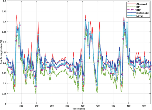
The comparison chart of the four network prediction effects is shown in Figure 5.

Figure 5. The forecast result of four methods.

The prediction accuracy of each method is shown in Table 1.

Table 1. Comparison of the performance indicators of the four methods.

Methods of prediction	MSE	NRMSE	MAPE/%	Train time (s)	Test time (µs)
BP	1321.5601	1.9825	12.8237	37.514	122.31
RBF	1002.2146	0.9312	8.9912	32.433	116.83
LSTM	712.45366	0.6619	6.3917	28.162	87.60
Multi-model	467.4468	0.4056	4.3379	23.092	31.12

It can be seen from Figure 5 and Table 1 that the prediction accuracy of the multi-model proposed in this paper is better than the three single-model prediction methods and the time spent on both training and testing is minimal.

In order to exclude contingencies and confirm the performance of the proposed method, the same method is used to average each of the above methods after 20 consecutive experiments, and the experimental results are shown in Table 2. The result is that the multi-model has better prediction performance.

Table 2. Comparison of the mean performance indicators of the four methods after 20 consecutive experiments.

Methods of prediction	MSE	NRMSE	MAPE/%
BP	1356.4701	2.0125	13.9276
RBF	1092.6734	1.0981	9.0124
LSTM	772.4611	0.7654	6.9667
Multi-model	481.9152	0.5031	4.5227

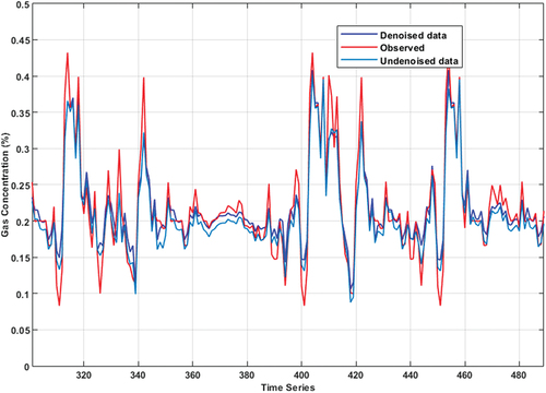
Further indications of the validity of the multi-model prediction approach are provided. Predictions were made using both un-denoised gas data and de-noised gas data.

The comparison chart of prediction effects of denoised and un-denoised gas data is shown in Figure 6.

Figure 6. Comparison of prediction effects of denoised and un-denoised gas data.

Discussion

The prediction results of the multi-model, BP, RBF and LSTM used in this paper are shown in Figure 5, and the performance indexes of the four methods are shown in Table 1. The prediction methods based on EMD denoising and multi-model had the lowest values of MSE, NRMSE and MAPE and the best prediction results compared to the other three. The LSTM network, RBF network and BP neural network had the next worst prediction results. The reason of the experiment result is that LSTM has a memory network, and the prediction performance is better. RBF network has better generalization ability than BP network. RBF network can approximate any non-linear function with arbitrary precision and has global approximation ability. It can solve the local optimum problem of BP network. Therefore, RBF network has better prediction performance than BP network. In order to further verify the prediction performance of the proposed model methods, two sets of experiments are used to illustrate this paper. Experiment 1: This paper uses 20 consecutive experiments using the four prediction methods to demonstrate the advantages of multi-model prediction using average performance metrics. Experiment 2: this paper uses gas data with and without noise to predict. The prediction results are shown in Figure 6 and the specific performance index values are shown in Table 3. It can be seen that even if there are no noise data, the performance indicators of the method adopted in this paper are very good and better than the three comparison methods in this paper.

Table 3. Comparison of forecast error of two methods.

Methods of prediction	MSE	NRMSE	MAPE/%
Multi-model-Noised	532.4685	0.4823	5.2237
Multi-model	467.4468	0.4056	4.3379

The prediction accuracy of the multi-model proposed in this paper is better than those of the three single-model prediction methods. By analyzing the reason, BP, RBF and LSTM networks belong to the single model prediction model, and the fully connected structure-induced model has strong coupling between hidden nodes in the learning process, which makes the model prediction accuracy poor. In addition, the gas concentration data with noise also affect the prediction accuracy of these three models to a certain extent. Firstly, the method proposed in this paper adopts the EMD method to self-adaptively de-noise the gas concentration time-series data containing noise, which can not only reduce the influence of noise on the prediction accuracy but also enhance the stability of the prediction results. At the same time, a hierarchical multi-model prediction model is used, which can select different sub-models for processing the data in different regions, and can process each data with multiple sub-sub-models and finally integrate it. Therefore, it not only avoids the influence of different regional data on the prediction model but also improves the prediction accuracy of the model.

Conclusion

Aiming at the problem of predicting the concentration of mine gas in the gas blending stage in the gas power generation process, a multi-model prediction model is proposed to predict the mine gas extraction. The method first aims at the problem that the measured gas concentration time-series data contain a lot of noise, and use the EMD method to decompose the time-series data into multiple independent IMF and residual terms. This process overcomes the influence of noise on the prediction model; secondly, this paper proposes a hierarchical multi-model prediction model, the model not only allows for the selection of different sub-models to handle data from different regions but each data is processed collaboratively by multiple sub-models in the model, improving the prediction accuracy of the model. Finally, the method proposed in this paper is used for the prediction of mine gas concentration time-series data, and satisfactory results are obtained, which improves the accuracy of gas blending control and provides a guarantee for the subsequent gas power generation process.

Acknowledgments

The authors of this paper would like to thank the referees for their valuable comments for the improvment of the manuscript. We also indicate there is no conflict of interest on this research paper.

Disclosure statement

No potential conflict of interest was reported by the author(s).

Additional information

Funding

This work is supported by the Basic Research plan of Natural Science Foundation of Shaanxi Coal Joint Fund (No. 2019JLZ-08); the Basic Research Plan of Nature Science in Shaanxi Province of China (No. 2020JM-522, 2021JM-396).

References

- Altan, A., S. Karasu, and E. Zio. 2021. A new hybrid model for wind speed forecasting combining long short-term memory neural network, decomposition methods and grey wolf optimizer. Applied Soft Computing 100:106996. doi:10.1016/j.asoc.2020.106996.
- Bo, C. Y., J. F. Qiao, and G. Yang. 2011. A multi-module cooperative neural network. CAAI Transactions on Intelligent Systems 6 (3):225–3792.
- Du, D., X. Jiang, H. Sun, and Z. Nie. 2019. An APSO-BP prediction modeling of malodorous gas in landfill based on historical data. Proceedings of the 2019 International Conference on Artificial Intelligence and Computer Science, Wuhan, Hubei, China, 390–93.
- Guo, S., and Y. Li. 2018. Prediction of underground gas concentration state based on data fusion. Journal of Xi’an University of Science and Technology 38 (3):506–14.
- Jia, P., and J. Deng. 2012. Coal mine gas concentration combination prediction model based on universal average operation. Zhongguo Anquan Kexue Xuebao 22 (6):41–46.
- Jia, P., H. Liu, S. Wang, and P. Wang. 2020. Research on a mine gas concentration forecasting model based on a GRU network. IEEE Access 8:38023–31. doi:10.1109/ACCESS.2020.2975257.
- Jin, G. G., and Y. D. Son. 2019. Design of a nonlinear PID controller and tuning rules for first-order plus time delay models. Studies in Informatics and Control 28 (2):157–66. doi:10.24846/v28i2y201904.
- Karasu, S., and A. Altan. 2022. Crude oil time series prediction model based on LSTM network with chaotic Henry gas solubility optimization. Energy 242:122964. doi:10.1016/j.energy.2021.122964.
- Karasu, S., A. Altan, S. Bekiros, and W. Ahmad. 2020. A new forecasting model with wrapper-based feature selection approach using multi-objective optimization technique for chaotic crude oil time series. Energy 212:118750. doi:10.1016/j.energy.2020.118750.
- Kim, H., R. Eykholt, and J. D. Salas. 1999. Nonlinear dynamics, delay times, and embedding windows. Physica D Nonlinear Phenomena 127 (1–2):48–60. doi:10.1016/S0167-2789(98)00240-1.
- Li, D., M. Han, and J. Wang. 2012. Chaotic time series prediction based on a novel robust echo state network. IEEE Transactions on Neural Networks and Learning Systems 23 (5):787–99. doi:10.1109/TNNLS.2012.2188414.
- Liu, Y., Q. Zhao, and W. Hao. 2015. Study of gas concentration prediction based on genetic algorithm and optimizing BP neural network. Mining Safety & Environmental Protection 42 (02):56–60.
- Li, B., E. Wang, Z. Shang, Z. Li, B. Li, X. Liu, H. Wang, Y. Niu, Q. Wu, and Y. Song. 2021. Deep learning approach to coal and gas outburst recognition employing modified AE and EMR signal from empirical mode decomposition and time-frequency analysis. Journal of Natural Gas Science and Engineering 90:103942. doi:10.1016/j.jngse.2021.103942.
- Nisbet, E. G., M. R. Manning, E. J. Dlugokencky, R. E. Fisher, D. Lowry, S. E. Michel, C. Lund Myhre, S. M. Platt, G. Allen, P. Bousquet, et al. 2019. Very strong atmospheric methane growth in the 4 years 2014–2017: Implications for the Paris agreement. Global biogeochemical cycles 33 (3):318–42. doi:10.1029/2018GB006009.
- Niu, Y., X. Song, Z. Li, E. Wang, Q. Liu, X. Zhang, G. Cai, and Q. Zhang. 2020. Experimental study and field verification of stability monitoring of gas drainage borehole in mining coal seam. Journal of Petroleum Science and Engineering 189:106985. doi:10.1016/j.petrol.2020.106985.
- Pang, Q., L. X. Tang, M. Z. Yuan, and X. P. Wang. 2012. The multi-model predictive control method research on the outlet temperature control of ethylene cracking furnace. Proceedings of the 31st Chinese Control Conference, IEEE, Hefei, China, 4044–49.
- Park, H. S., W. Pedrycz, and S. K. Oh. 2009. Granular neural networks and their development through context-based clustering and adjustable dimensionality of receptive fields. IEEE Transactions on Neural Networks 20 (10):1604–16. doi:10.1109/TNN.2009.2027319.
- Pedrycz, W. 1998. Conditional fuzzy clustering in the design of radial basis function neural networks. IEEE Transactions on Neural Networks 9 (4):601–12. doi:10.1109/72.701174.
- Perendeci, A., S. Arslan, S. S. Celebi, and A. Tanyolac. 2008. Prediction of effluent quality of an anaerobic treatment plant under unsteady state through ANFIS modeling with on-line input variables. Chemical Engineering Journal 145 (1):78–85. doi:10.1016/j.cej.2008.03.008.
- Pipino, H. A., C. A. Cappelletti, and E. J. Adam. 2021. Adaptive multi-model predictive control applied to continuous stirred tank reactor. Computers & Chemical Engineering 145:107195. doi:10.1016/j.compchemeng.2020.107195.
- Prakash, U. M., K. Kottursamy, K. Cengiz, U. Kose, and B. T. Hung. 2021. 4x-expert systems for early prediction of osteoporosis using multi-model algorithms. Measurement 180:109543. doi:10.1016/j.measurement.2021.109543.
- Qiao, M., X. Ma, J. Lan, and Y. Wang. 2011. Time-series gas prediction model using LS-SVR within a Bayesian framework. Mining Science and Technology (China) 21 (1):153–57. doi:10.1016/j.mstc.2010.12.012.
- Sohani, A., H. Sayyaadi, C. Cornaro, M. H. Shahverdian, M. Pierro, D. Moser, M. H. Doranehgrad, N. Karimi, and L. K. Li. 2022. Using machine learning in photovoltaics to create smarter and cleaner energy generation systems: A comprehensive review. Journal of Cleaner Production 364:132701. doi:10.1016/j.jclepro.2022.132701.
- Soltani, S. 2002. On the use of the wavelet decomposition for time series prediction. Neurocomputing 48 (1–4):267–77.
- Song, Y., S. Yang, X. Hu, W. Song, N. Sang, J. Cai, and Q. Xu. 2019. Prediction of gas and coal spontaneous combustion coexisting disaster through the chaotic characteristic analysis of gas indexes in goaf gas extraction. Process Safety and Environmental Protection 129:8–16. doi:10.1016/j.psep.2019.06.013.
- Wang, W., H. Wang, B. Zhang, S. Wang, and W. Xing. 2021. Coal and gas outburst prediction model based on extension theory and its application. Process Safety and Environmental Protection 154:329–37. doi:10.1016/j.psep.2021.08.023.
- Yin, G. Z., M. H. Li, and W. P. LI. 2013. Model of coal gas permeability prediction based on improved BP neural network. Journal of China Coal Society 38 (7):1179–84.
- Zeng, J., and Q. Li. 2021. Research on prediction accuracy of coal mine gas emission based on grey prediction model. Processes 9 (7):1147. doi:10.3390/pr9071147.
- Zhang, Q. 2019. Process technology and design research of intelligent mixing system for low concentration gas based on S7-1200. Mining Safety & Environmental Protection 46 (2):79–83.
- Zhang, T., S. Song, S. Li, L. Ma, S. Pan, and L. Han. 2019. Research on gas concentration prediction models based on LSTM multidimensional time series. Energies 12 (1):161. doi:10.3390/en12010161.
- Zhou, X. L., G. Zhang, C. Lyu, and H. Huang. 2017. A grey model for predicting the gas content in the deep coal seam and its application via the neural network of the difference radial basis function. Journal Safety Environment 17:2050–55.