An online self-adaptive RBF network algorithm based on the Levenberg-Marquardt algorithm

ABSTRACT

Aiming at the problem that the Levenberg-Marquardt (LM) algorithm can not train online radial basis function (RBF) neural network and the deficiency in the RBF network structure design methods, this paper proposes an online self-adaptive algorithm for constructing RBF neural network (OSA-RBFNN) based on LM algorithm. Thus, the ideas of the sliding window method and online structure optimization methods are adopted to solve the proposed problems. On the one hand, the sliding window method enables the RBF network to be trained online by the LM algorithm making the RBF network more robust to the changes in the learning parameters and faster convergence compared with the other investigated algorithms. On the other hand, online structure optimization can adjust the structure of the RBF network based on the information of training errors and hidden nodes to track the non-linear time-varying systems, which helps to maintain a compact network and satisfactory generalization ability. Finally, verified by simulation analysis, it is demonstrated that OSA-RBFNN exhibits a compact RBF network.

Introduction

RBF neural network has been extensively applied to industrial control, pattern classification, signal processing, modeling of non-linear systems and other areas, as it has the ability of strong non-linear fitting, faster convergence, strong robustness, and is not easy to lead to local minima (Gao 2022; La Rosa Centeno et al. 2018; Zhang et al. 2020; Zhou, Oh, and Qiu 2022). Structure constructing methods and parameters tuning algorithms are the keys to construct RBF neural networks (Gu, Tok, and Yu 2018). Structural constructing is the strategy used to determine the number of hidden nodes in the RBF network; Parameter tuning is how to adjust three parameters in this network (Kadakadiyavar, Ramrao, and Singh 2020).

In recent years, considerable advancement has been proposed in the structural construction of the RBF network. The first algorithm dynamically adapts the weights of the participating kernels using the gradient descent method thereby alleviating the need for predetermined weights (Khan et al. 2017). The second method realizes online modeling by combing the advantages of the sliding window strategy and clustering algorithm (Jia, Li, and Qiao 2022). The novel algorithm provides better performance such as faster convergence rate, better local minima, and resilience against leading to poor local minima. It is a multi-kernel radial basis function neural network in which every base kernel has its weight (Atif et al. 2022).

Regarding architectural optimization for RBF neural networks, the most classic online algorithms are resource-allocating network (RAN), minimal resource allocating network (MRAN), and generalized growing and pruning radial basis function (GGAP-RBF). The principles mentioned above of algorithms both design the network online to meet the accuracy requirements, maintain a compact structure, and improve its generalization performance (Meng, Zhang, and Qiao 2021). Therefore, it is important to design an online neural network. However, these algorithms have deficiencies in networks.

John Platt (Platt 1991) presented RAN to test each training sample continuously. When the new training sample meets the ”‘novelty’,” a new node is allocated to the training sample. However, once the hidden nodes are added, they will not be pruned in the algorithm. Therefore, redundant hidden nodes will inevitably appear in this network for complex online learning tasks, affecting the network’s generalization performance.

To address the mentioned problems, Lu Y W et al. (Lu, Sundararajan, and Saratchandran 1997) proposed that MRAN is improved by RAN. On the one hand, if the deviation of the current network for multiple consecutive training samples is too large, add a hidden node; if several consecutive training samples cannot activate a hidden node, prune the node (Jia, Li, and Qiao 2022). To a certain extent, MRAN can obtain a compact network model. On the other hand, it also has blindness with adding nodes, because the center of the kernel function is determined randomly. Thereby it results in the poor robustness and generalization performance of the algorithms (Arif, Ray Chaudhuri, and Ray et al. 2009).

Based on the poor performance of the MRAN network. In (Li, Chen, and Huang 2006), GGAP-RBF neural network links the required learning accuracy to the significance of neurons in the learning algorithm to realize a compact RBF network. But the neural network needs to initialize the network parameters based on all samples, thus it is difficult to realize an optimal online algorithm for the RBF network.

The RAN, MRAN, and GGAP-RBF algorithms use the gradient descent method for the parameters learning algorithm. The gradient descent method is the first-order algorithm. The main problem of the first-order algorithm is slow convergence, and it is easy to lead to the local minimum of the curved error surface. In these situations, second-order algorithms are superior. The Levenberg-Marquardt (LM) algorithm (Houcine Bergou, Diouane, and Kungurtsev 2020) is a second-order algorithm, which is a mix of the Steepest Gradient Method and Gauss–Newton method. When the gradient of the error surface is small, the LM algorithm is similar to the Steepest Gradient Method. When the gradient of the error surface is large, the LM algorithm is similar to the Gauss–Newton method. LM can estimate the learning rate of each gradient under the curved error surface according to the Hessian matrix. The LM algorithm is efficient for training neural networks compared to the first-order algorithm (Wilamowski and Yu 2010).

The error correction (ErrCor) algorithm (Hao et al. 2014) applies the LM algorithm to train the RBF network, and after each iteration, it turns out that a much better learning ability of the RBF network can be obtained when adding a new RBF node at the location of the highest error peak or lowest error valley. This algorithm has strong robustness and can design a compact network (Xi et al. 2018). However, it is an offline design and difficult to apply to non-linear time-varying systems.

Based on previous research, according to the above-mentioned problems, we propose an online self-adaptive algorithm for the RBF network based on the LM algorithm. The algorithm builds a sliding window and uses the LM algorithm to train the RBF network. During the training process, it can add, prune or merge hidden nodes according to the training error information and the relevant information of each hidden node, which makes the RBF network structure compact in the learning process, and then ensures the generalization performance of the RBF network. Using the sliding window method can achieve the online application of the LM algorithm and make the RBF network more robust to changes in learning parameters and easier to converge. Finally, the performance of OSA-RBFNN is verified by simulation experiments.

The remainder of this paper is organized as follows. Section 1 introduces RBF network briefly. In Section 2, an online self-adaptive optimal algorithm for the RBF network is proposed in detail. Section 3 evaluates OSA-RBFNN through simulation analysis. Finally, the study is concluded in Section 4.

Materials and Methods

RBF Network

The RBF network comprises three feedforward network layers: the input layer, the hidden layer, and the output layer. The weight connection from the input layer to the hidden layer is fixed at 1. Without loss of generality, set the RBF network structure is I-H-1, that is I input nodes, H hidden nodes, and one output node. The structure is given in Figure 1.

Figure 1. Structure of RBF networks.

Set $x_p=[x_{p,1},x_{p.2},\dots ,x_{p,I}]$ is the pth I dimensional sample in the RBF network, the output of the hth hidden node is as Equation (1)(1) ${\varphi }_p(x_p)=exp\left(-\frac{\parallel x_p-c_h{\parallel }^2}{{\sigma }_h}\right)$(1) :

(1) ${\varphi }_p(x_p)=exp\left(-\frac{\parallel x_p-c_h{\parallel }^2}{{\sigma }_h}\right)$(1)

Where$c_h$and${\sigma }_h$are the center vector of the hth RBF node and its width, respectively, $\parallel \cdot \parallel$denotes Euclidean distance.

The output of the network for the pth sample is as Equation (2)(2) $O_p=\sum _{h=1}^H{w}_h{\varphi }_p\left(x_p\right)+w_0$(2) :

(2) $O_p=\sum _{h=1}^H{w}_h{\varphi }_p\left(x_p\right)+w_0$(2)

where$w_h$denotes the weight connecting between the hth hidden node and the output node,$w_0$is bias.

LM Algorithm

The LM algorithm is a second-order algorithm successfully applied to the back propagation (BP) network. In terms of the LM algorithm training RBF network, the paper (Wilamowski and Yu 2010) improved the LM algorithm. On this basis, the paper (Hao et al. 2014) proposed an error correction (ErrCor) algorithm to construct the RBF network structure based on the peak of error training. This algorithm belongs to the growth algorithm and can design a compact RBF network structure.

When the LM algorithm trains the RBF network, the parameter update rule is as Equation (3)(3) ${\mathrm{\Delta }}_{k+1}={\mathrm{\Delta }}_k-{\left(Q_k+{\mu }_{k}I\right)}^{-1}{g}_k$(3) .

(3) ${\mathrm{\Delta }}_{k+1}={\mathrm{\Delta }}_k-{\left(Q_k+{\mu }_{k}I\right)}^{-1}{g}_k$(3)

Where$\mathrm{\Delta }$denotes tuning parameter in RBF network (including centers c, widths σ, and the output weights w); Q denotes Quasi-Hessian matrix; I is the identity matrix; $\mu$is the learning coefficient; g is the gradient vector.

The training error$e_p$is calculated as the desired output$y_p$ and actual output$o_p$, it is shown in Equation (4)(4) $e_p=y_p-o_p.$(4) .

(4) $e_p=y_p-o_p.$(4)

The element$j_{p,n}$of the nth row of the Jacobian matrix can be calculated by Equation (5)(5) $j_{p,n}=\frac{\mathrm{\partial }{e}_p}{\mathrm{\partial }{\mathrm{\Delta }}_n},$(5) .

(5) $j_{p,n}=\frac{\mathrm{\partial }{e}_p}{\mathrm{\partial }{\mathrm{\Delta }}_n},$(5)

Where n is three tuning parameters in this RBF network.

The gradient vector g is calculated through the sum of sub-vector ${\eta }_p$in Equation (6)(6) $\mathrm{g}=\sum _{p=1}^P{\eta }_p$(6) .

(6) $\mathrm{g}=\sum _{p=1}^P{\eta }_p$(6)

and sub-vector ${\eta }_p$ is calculated as Equation (7)(7) ${\eta }_p=j_p^T{e}_p$(7) .

(7) ${\eta }_p=j_p^T{e}_p$(7)

Where $j_p$ is the row of Jacobian matrix and $e_p$ is calculated as Equation (4)(4) $e_p=y_p-o_p.$(4) .

The calculation of quasi-Hessian matrix Q is transformed to the sum of sub-matrices in Equation (8)(8) $Q=\sum _{p=1}^P{q}_p,q_p=j_p^T{j}_p$(8) .

(8) $Q=\sum _{p=1}^P{q}_p,q_p=j_p^T{j}_p$(8)

For a given p training sample, and considering the tuning parameter$w_h,{\mathrm{c}}_{h,i}$, and${\sigma }_h$under the RBF network, the Jacobian row elements is calculated by Equation (9)(9) $j_p=\left[\begin{array}{c}\frac{\mathrm{\partial }{e}_p}{\mathrm{\partial }{\omega }_0},\frac{\mathrm{\partial }{e}_p}{\mathrm{\partial }{\omega }_1}\dots \frac{\mathrm{\partial }{e}_p}{\mathrm{\partial }{\omega }_h}\dots \frac{\mathrm{\partial }{e}_p}{\mathrm{\partial }{\omega }_H},\frac{\mathrm{\partial }{e}_p}{\mathrm{\partial }{c}_{1,1}}\dots \frac{\mathrm{\partial }{e}_p}{\mathrm{\partial }{c}_{1,i}}\dots \frac{\mathrm{\partial }{e}_p}{\mathrm{\partial }{c}_{1,I}}\dots \frac{\mathrm{\partial }{e}_p}{\mathrm{\partial }{c}_{h,1}}\dots \\ \frac{\mathrm{\partial }{e}_p}{\mathrm{\partial }{c}_{h,i}}\dots \frac{\mathrm{\partial }{e}_p}{\mathrm{\partial }{c}_{H,1}}\dots \frac{\mathrm{\partial }{e}_p}{\mathrm{\partial }{c}_{H,i}}\dots \frac{\mathrm{\partial }{e}_p}{\mathrm{\partial }{c}_{H,I}},\frac{\mathrm{\partial }{e}_p}{\mathrm{\partial }{\sigma }_1}\dots \frac{\mathrm{\partial }{e}_p}{\mathrm{\partial }{\sigma }_h}\dots \frac{\mathrm{\partial }{e}_p}{\mathrm{\partial }{\sigma }_H}\end{array}\right].$(9) .

(9) $j_p=\left[\begin{array}{c}\frac{\mathrm{\partial }{e}_p}{\mathrm{\partial }{\omega }_0},\frac{\mathrm{\partial }{e}_p}{\mathrm{\partial }{\omega }_1}\dots \frac{\mathrm{\partial }{e}_p}{\mathrm{\partial }{\omega }_h}\dots \frac{\mathrm{\partial }{e}_p}{\mathrm{\partial }{\omega }_H},\frac{\mathrm{\partial }{e}_p}{\mathrm{\partial }{c}_{1,1}}\dots \frac{\mathrm{\partial }{e}_p}{\mathrm{\partial }{c}_{1,i}}\dots \frac{\mathrm{\partial }{e}_p}{\mathrm{\partial }{c}_{1,I}}\dots \frac{\mathrm{\partial }{e}_p}{\mathrm{\partial }{c}_{h,1}}\dots \\ \frac{\mathrm{\partial }{e}_p}{\mathrm{\partial }{c}_{h,i}}\dots \frac{\mathrm{\partial }{e}_p}{\mathrm{\partial }{c}_{H,1}}\dots \frac{\mathrm{\partial }{e}_p}{\mathrm{\partial }{c}_{H,i}}\dots \frac{\mathrm{\partial }{e}_p}{\mathrm{\partial }{c}_{H,I}},\frac{\mathrm{\partial }{e}_p}{\mathrm{\partial }{\sigma }_1}\dots \frac{\mathrm{\partial }{e}_p}{\mathrm{\partial }{\sigma }_h}\dots \frac{\mathrm{\partial }{e}_p}{\mathrm{\partial }{\sigma }_H}\end{array}\right].$(9)

Integrating Equations (1)(1) ${\varphi }_p(x_p)=exp\left(-\frac{\parallel x_p-c_h{\parallel }^2}{{\sigma }_h}\right)$(1) , (2(2) $O_p=\sum _{h=1}^H{w}_h{\varphi }_p\left(x_p\right)+w_0$(2) ), and (4(4) $e_p=y_p-o_p.$(4) ), with the differential chain rule, the Jacobian row of the pth training sample in (6) can be rewritten as Equations (10)(10) $\frac{\mathrm{\partial }{e}_p}{\mathrm{\partial }{\omega }_h}=-{\phi }_h\left(X_p\right),\frac{\mathrm{\partial }{e}_p}{\mathrm{\partial }{\omega }_0}=-1,$(10) ~(12)(12) $\frac{\mathrm{\partial }{e}_p}{\mathrm{\partial }{\sigma }_h}=-\frac{{\omega }_h{\phi }_h\left(X_p\right)\parallel X_p-c_h{\parallel }^2}{{\sigma }_h^2}.$(12) .

(10) $\frac{\mathrm{\partial }{e}_p}{\mathrm{\partial }{\omega }_h}=-{\phi }_h\left(X_p\right),\frac{\mathrm{\partial }{e}_p}{\mathrm{\partial }{\omega }_0}=-1,$(10)

(11) $\frac{\mathrm{\partial }{e}_p}{\mathrm{\partial }{c}_{h,i}}=-\frac{2{\omega }_h{\phi }_h\left(X_p\right)\left(x_{p,i}-c_{h,i}\right)}{{\sigma }_h},$(11)

(12) $\frac{\mathrm{\partial }{e}_p}{\mathrm{\partial }{\sigma }_h}=-\frac{{\omega }_h{\phi }_h\left(X_p\right)\parallel X_p-c_h{\parallel }^2}{{\sigma }_h^2}.$(12)

Integrating Equations (10)(10) $\frac{\mathrm{\partial }{e}_p}{\mathrm{\partial }{\omega }_h}=-{\phi }_h\left(X_p\right),\frac{\mathrm{\partial }{e}_p}{\mathrm{\partial }{\omega }_0}=-1,$(10) ~(12(12) $\frac{\mathrm{\partial }{e}_p}{\mathrm{\partial }{\sigma }_h}=-\frac{{\omega }_h{\phi }_h\left(X_p\right)\parallel X_p-c_h{\parallel }^2}{{\sigma }_h^2}.$(12) ), all the elements of Jacobian row of the jth can be calculated. For all input samples, all elements of the Jacobian matrix can be calculated. Quasi-Jacobian matrix Q and gradient vector g are obtained by Equations (6)(6) $\mathrm{g}=\sum _{p=1}^P{\eta }_p$(6) ~(8(8) $Q=\sum _{p=1}^P{q}_p,q_p=j_p^T{j}_p$(8) ). To apply the update Equation (3)(3) ${\mathrm{\Delta }}_{k+1}={\mathrm{\Delta }}_k-{\left(Q_k+{\mu }_{k}I\right)}^{-1}{g}_k$(3) for parameter adjustment.

Online Self-Adaptive Optimal Algorithm for RBF Network(OSA-RBFNN)

Although the LM algorithm is a effective algorithm for training neural networks at present, the LM algorithm can only be used in batch processing when training the RBF network. Hence, the ErrCor algorithm is an offline algorithm for designing the RBF network structure and cannot be performed online, it is not easy to apply to non-linear time-varying systems. In addition, since the RAN, MRAN, and GGAP-RBF online algorithms all use the latest single sample to train the RBF network, it leads to a poor local optimum, and if it has a sample noise impact on learning, it will result in the poor accuracy of learning. For online modeling, the reasonable method is to use the latest multiple samples to dynamically adjust the network parameters during the learning process (Arif, Ray Chaudhuri, and Ray et al. 2009).

The mentioned problems can be worked out by the using sliding window method in this paper (Pedro and Ruano 2009). The sliding window is a “FIFO” (First In First Out) queue of a fixed length. The elements of the queue are the online input sample by the entry window in chronological order. Sets online input sample is$\left(x_n,y_n\right)$, thus the elements in the sliding window of the length of L denotes$\left[\left(x_i,y_i\right),\left(x_{i+1},y_{i+1}\right),\dots ,\left(x_{i+L-1},y_{i+l-1}\right)\right].$When a new sample arrives, the sample in this window are updated by including the latest sample and eliminating the oldest. All the samples in the sliding window are the RBF network training sample.

As above, when using the sliding window method, and applying the LM algorithm to training the RBF network, the target function of RBF network learning is as Equation (13)(13) ${\mathrm{e}}_L=\sum _{i=1}^L{\beta }_i{\left(y_i-o_i\right)}^2.$(13) .

(13) ${\mathrm{e}}_L=\sum _{i=1}^L{\beta }_i{\left(y_i-o_i\right)}^2.$(13)

Where L is the length of the sliding window;$y_i$and$o_i$denotes desired outputs and actual outputs of the ith sample in the sliding window;${\beta }_i$is a forgetting factor, and it can be shown as Equation (14)(14) ${\beta }_i=\frac{2i}{L\left(L+1\right)},\sum _i^L{\beta }_i=1.$(14) .

(14) ${\beta }_i=\frac{2i}{L\left(L+1\right)},\sum _i^L{\beta }_i=1.$(14)

Based on Equations (13)(13) ${\mathrm{e}}_L=\sum _{i=1}^L{\beta }_i{\left(y_i-o_i\right)}^2.$(13) and (14(14) ${\beta }_i=\frac{2i}{L\left(L+1\right)},\sum _i^L{\beta }_i=1.$(14) ), the latest sample has a large amount of information from online learning, the weighting coefficients of the latest sample of the sliding window are more significant than under the old sample, its weighting coefficients are small.

The online self-adaptive optimal algorithm for the RBF network in this paper has three options: adding, pruning, and merging network hidden nodes.

Adding the hidden nodes. For the process of online training, the maximum error of the samples in each sliding window is detected and recorded. Therefore, one hidden node is added to the hidden layer and regarded with its kernel function center as the training sample corresponding to the currently recorded maximum training error when the RBF network is trained to a certain step, and the root mean square error (RMSE) of the training samples in the sliding window does not reach the target value. The RMSE of the training sample in the sliding window is shown in Equation (15)(15) $e_{rmse}=\sqrt{\frac{\sum _{i=1}^L{\beta }_i{\left(y_i-o_i\right)}^2}{L}.}$(15) .

(15) $e_{rmse}=\sqrt{\frac{\sum _{i=1}^L{\beta }_i{\left(y_i-o_i\right)}^2}{L}.}$(15)

Pruning the hidden nodes. If such inactive hidden nodes can be detected and removed as learning progresses, it will mean that the hidden node will lose the ability of learning. The criterion for judging whether the hidden node is activated is in Equation (16)(16) ${\varphi }_h^k\left(x_k\right)=w_h^{k}exp\left(-\frac{\parallel x_k-c_h{\parallel }^2}{{\sigma }_h}\right),r_h^k=\parallel \frac{{\varphi }_h^k}{{\varphi }_{max}^k}\parallel .$(16) (Lu, Sundararajan, and Saratchandran 1997).

(16) ${\varphi }_h^k\left(x_k\right)=w_h^{k}exp\left(-\frac{\parallel x_k-c_h{\parallel }^2}{{\sigma }_h}\right),r_h^k=\parallel \frac{{\varphi }_h^k}{{\varphi }_{max}^k}\parallel .$(16)

where${\varphi }_h^k$is the output of the hth hidden node at time k, $w_h^k$is the weight connecting from hidden node h to output node at k time. $r_h^k$is the normalized output of the hth hidden nodes at time k, ${\varphi }_{max}^k$is the value of the largest absolute value among the outputs of all hidden nodes at k time. For multiple consecutive training samples, if $r_h^k$is less than a threshold$\delta$, it will be pruned.

Merging the hidden nodes. In the process of learning, if the distance of the center and the width are close significantly between the two hidden nodes under the RBF network, according to the characteristics of the local response characteristics of the hidden nodes of the RBF network, the function of the two nodes is almost identical. Thus, we will merge the two hidden nodes into one. This operation will not only simplify the RBF network structure but make no difference to the learning performance of the current network. The relevant parameters can be set as Equation(17)(17) $\left\{\begin{array}{c}{w}_i=w_i+w_j,\\ c_i=\left(c_i+c_j\right)/2,\\ {\sigma }_i=max\left({\sigma }_i,{\sigma }_j\right).\end{array}\right.$(17) .

(17) $\left\{\begin{array}{c}{w}_i=w_i+w_j,\\ c_i=\left(c_i+c_j\right)/2,\\ {\sigma }_i=max\left({\sigma }_i,{\sigma }_j\right).\end{array}\right.$(17)

Using the sliding window method can achieve the online application of the LM algorithm and make the RBF network more robust to changes in learning parameters and faster convergence. The structure optimization algorithm combines the advantages of RAN, MRAN, and GGAP-RBF, and it also overcomes their shortcomings. One hidden node is added to the hidden layer and regarded as its kernel function center as the training sample corresponding to the currently recorded maximum training error. It can not only reduce the training error but avoid adding hidden nodes randomly.

Considering the aforementioned problems, an online self-adaptive optimal algorithm for the RBF network can be obtained and it is shown in Table 1.

Table 1. Algorithmic depiction of OSA-RBFNN.

Initialization set the length of the sliding window L there is one hidden node in the network for k = 1:NMAX move new samples $\left(x_k,y_k\right)$ to the sliding windows, then remove the first sample calculate $e_{rmse}$ of the sample in the current sliding window using Equation (15)(15) $e_{rmse}=\sqrt{\frac{\sum _{i=1}^L{\beta }_i{\left(y_i-o_i\right)}^2}{L}.}$(15) (step=1) for step = 2:max_step find maximum of abs error of $e_{rmse}$ if the fixed training steps is reached and $e_{rmse}>e_{obj}$ ($e_{obj}$ is the target value of the network training error) create a new hidden node at the location of maximum error by setting weight the width of the new RBF node to 1. calculate Jacobian vector $j_p$ using Equations (9)(9) $j_p=\left[\begin{array}{c}\frac{\mathrm{\partial }{e}_p}{\mathrm{\partial }{\omega }_0},\frac{\mathrm{\partial }{e}_p}{\mathrm{\partial }{\omega }_1}\dots \frac{\mathrm{\partial }{e}_p}{\mathrm{\partial }{\omega }_h}\dots \frac{\mathrm{\partial }{e}_p}{\mathrm{\partial }{\omega }_H},\frac{\mathrm{\partial }{e}_p}{\mathrm{\partial }{c}_{1,1}}\dots \frac{\mathrm{\partial }{e}_p}{\mathrm{\partial }{c}_{1,i}}\dots \frac{\mathrm{\partial }{e}_p}{\mathrm{\partial }{c}_{1,I}}\dots \frac{\mathrm{\partial }{e}_p}{\mathrm{\partial }{c}_{h,1}}\dots \\ \frac{\mathrm{\partial }{e}_p}{\mathrm{\partial }{c}_{h,i}}\dots \frac{\mathrm{\partial }{e}_p}{\mathrm{\partial }{c}_{H,1}}\dots \frac{\mathrm{\partial }{e}_p}{\mathrm{\partial }{c}_{H,i}}\dots \frac{\mathrm{\partial }{e}_p}{\mathrm{\partial }{c}_{H,I}},\frac{\mathrm{\partial }{e}_p}{\mathrm{\partial }{\sigma }_1}\dots \frac{\mathrm{\partial }{e}_p}{\mathrm{\partial }{\sigma }_h}\dots \frac{\mathrm{\partial }{e}_p}{\mathrm{\partial }{\sigma }_H}\end{array}\right].$(9) ~(12(12) $\frac{\mathrm{\partial }{e}_p}{\mathrm{\partial }{\sigma }_h}=-\frac{{\omega }_h{\phi }_h\left(X_p\right)\parallel X_p-c_h{\parallel }^2}{{\sigma }_h^2}.$(12) ) calculate sub quasi-Hessian matrix $q_p=j_p^T{j}_p$, and gradient vector ${\eta }_p=j_p^T{e}_p$ if check the hidden nodes and the node cannot activate prune the hidden node end if check redundant hidden nodes in the RBF network, and the Euclidean distance between the center of two hidden nodes is less than the threshold. merge the two hidden nodes using Equation (17)(17) $\left\{\begin{array}{c}{w}_i=w_i+w_j,\\ c_i=\left(c_i+c_j\right)/2,\\ {\sigma }_i=max\left({\sigma }_i,{\sigma }_j\right).\end{array}\right.$(17) end end calculate quasi-Hessian matrix Q using Equation (8)(8) $Q=\sum _{p=1}^P{q}_p,q_p=j_p^T{j}_p$(8) ;Using Equations (6)(6) $\mathrm{g}=\sum _{p=1}^P{\eta }_p$(6) and (7(7) ${\eta }_p=j_p^T{e}_p$(7) ) to calculate the gradient vector g. update RBF network parameters using Equation (3)(3) ${\mathrm{\Delta }}_{k+1}={\mathrm{\Delta }}_k-{\left(Q_k+{\mu }_{k}I\right)}^{-1}{g}_k$(3) ; calculate new output using Equation (16)(16) ${\varphi }_h^k\left(x_k\right)=w_h^{k}exp\left(-\frac{\parallel x_k-c_h{\parallel }^2}{{\sigma }_h}\right),r_h^k=\parallel \frac{{\varphi }_h^k}{{\varphi }_{max}^k}\parallel .$(16) , and sign the state of the node. calculate RMSE(step) while $e_{rmse}$ of the sample in the current sliding window is not reduced adjust the ${\mu }_k$ parameter using Equation (3)(3) ${\mathrm{\Delta }}_{k+1}={\mathrm{\Delta }}_k-{\left(Q_k+{\mu }_{k}I\right)}^{-1}{g}_k$(3) endwhile ($e_{rmse}$ is not reduced) if RMSE(step)<desired error, then break endfor(max_step) if RMSE(k)<desired error, then break(new RBF node loop) endfor(main loop)

Results and Discussion

Computational Complexity Analysis

In the subsection, we compare the computation complexity of the traditional RBF neural network algorithm with OSA-RBFNN.

To build a compact RBF neural network structure, we adopt the sliding window method based on the LM algorithm to optimize the structure by adjusting parameters continuously. RAN, MRAN, and GGAP algorithms all use the gradient descent method, while OSA-RNFNN uses the LM algorithm for training optimization. Let m denote the number of iterations required to reach the object training error, and s denote the training step.

The gradient descent method has the characters of slow convergence and a large number of iterations, the time complexity of one iteration can be approximated as$O(n)$. Thus, the computational complexity of training can be approximated as$O(m\ast s\ast n)$. While the LM algorithm has fast convergence and a small number of iterations, and one iteration time complexity is $O(n^3)$, the computational complexity can be approximated as$O(m\ast s\ast n^3)$. For the above-mentioned computational complexity, it is shown that the gradient descent method is better than the LM algorithm. However, for the RBF neural network structure, the LM algorithm can calculate the learning rate of each gradient under the curved error surface according to the Hessian matrix to obtain the optima compared to the gradient descent method. It will reduce the number of iterations largely. And OSA-RBFNN based on the LM algorithm uses the latest single sample to adjust parameters dynamically, it can reduce the training step and the training iterations to reach the object training error. Thus, the computational complexity of the LM algorithm is superior to the gradient descent method for OSA-RBFNN.

Non-Linear Function Approximation

We proposed OSA-RBFNN for constructing minimal RBF structure. According to Equation (1)(1) ${\varphi }_p(x_p)=exp\left(-\frac{\parallel x_p-c_h{\parallel }^2}{{\sigma }_h}\right)$(1) , we build a non-linear function in Equation (18)(18) $y\left(x\right)=exp\left[-\frac{{\left(x_1-0.3\right)}^2+{\left(x_2-0.2\right)}^2}{0.01}\right]+exp\left[-\frac{{\left(x_1-0.7\right)}^2+{\left(x_2-0.2\right)}^2}{0.01}\right]+exp\left[-\frac{{\left(x_1-0.1\right)}^2+{\left(x_2-0.5\right)}^2}{0.02}\right]+exp\left[-\frac{{\left(x_1-0.9\right)}^2+{\left(x_2-0.5\right)}^2}{0.01}\right]+exp\left[-\frac{{\left(x_1-0.3\right)}^2+{\left(x_2-0.8\right)}^2}{0.01}\right]+exp\left[-\frac{{\left(x_1-0.7\right)}^2+{\left(x_2-0.8\right)}^2}{0.01}\right]$(18) which consists of six exponential Gaussian functions (Yingwei, Sundararajan, and Saratchandran 1997). The function is the summation of six Gaussian exponential functions; thus, the RBF network should have six nodes with Gaussian functions in its hidden layer. In Figure 2, “△” indicates the true positions of hidden unit centers from non-linear function, and the circles represent the estimated positions of centers obtained from the minimal RBF network.

Figure 2. The attribution of the true and estimated centers.

(18) $y\left(x\right)=exp\left[-\frac{{\left(x_1-0.3\right)}^2+{\left(x_2-0.2\right)}^2}{0.01}\right]+exp\left[-\frac{{\left(x_1-0.7\right)}^2+{\left(x_2-0.2\right)}^2}{0.01}\right]+exp\left[-\frac{{\left(x_1-0.1\right)}^2+{\left(x_2-0.5\right)}^2}{0.02}\right]+exp\left[-\frac{{\left(x_1-0.9\right)}^2+{\left(x_2-0.5\right)}^2}{0.01}\right]+exp\left[-\frac{{\left(x_1-0.3\right)}^2+{\left(x_2-0.8\right)}^2}{0.01}\right]+exp\left[-\frac{{\left(x_1-0.7\right)}^2+{\left(x_2-0.8\right)}^2}{0.01}\right]$(18)

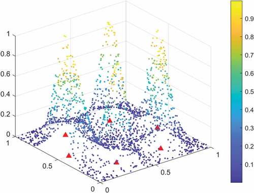
The aim is to construct a minimal RBF network using the method to approximate the function with small error. For this approximation, 2000 training samples$\left(\left(x_1,x_2\right),y\right)$were generated randomly, $\left(x_1,x_2\right)$and y present input and output, $x_i\in \left(0,1\right),i\in \left\{1,2\right\}.$And set the length of sliding window L is equal to 20.

Because of the randomness of the training results, we try running the experiment 20 times independently. The algorithm generated six hidden nodes, similar to the non-linear function, by training 16 times. In other times, we got seven hidden nodes. From Table 2, the centers, widths, and output weights for the non-linear function in the hidden nodes are quite close to the true values. Thus, OSA-RBFNN can accurately approximate the nonlinear function with minimal network size.

Table 2. Performance comparison of true and estimated value on object function.

True center	(0.3,0.2)	(0.7,0.2)	(0.1,0.5)	(0.9,0.5)	(0.3,0.8)	(0.7,0.8)
Estimated center	(0.3110, 0.2000)	(0.6798, 0.1993)	(0.0988, 0.5000)	(0.8799, 0.5103)	(0.3000, 0.7994)	(0.6981, 0.8022)
True width	0.1	0.1	0.144	0.144	0.1	0.1
Estimated width	0.0998	0.0999	0.1425	0.1496	0.0992	0.0995
True weight	1	1	1	1	1	1
Estimated weight	1.0299	1.0073	1.0200	0.9887	1.0021	1.0003

Non-Linear Time-Varying System Identification

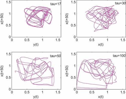
We choose a benchmark problem Mackey-Glass (MG) chaotic time series (Harpham and Dawson 2006; Jiang et al. 2022) generated by the differential delay Equation (19)(19) $\frac{dx}{dt}=\frac{0.2x(t-\tau )}{1+x^{10}\left(t-\tau \right)}-0.1x\left(t\right).$(19) to test the ability of OSA-RBFNN for non-linear time-varying system identification.

(19) $\frac{dx}{dt}=\frac{0.2x(t-\tau )}{1+x^{10}\left(t-\tau \right)}-0.1x\left(t\right).$(19)

And we use the input vector $\left[x(t)\hspace{0.17em}x(t-6)\hspace{0.17em}x(t-12)\hspace{0.17em}x(t-18)\right]$ to predict the output vector$x(t+50)$. Equation (19)(19) $\frac{dx}{dt}=\frac{0.2x(t-\tau )}{1+x^{10}\left(t-\tau \right)}-0.1x\left(t\right).$(19) is a static chaotic time series under the condition that τ is constant. We set τ equal to 17, 30, 50, and 100 separately to test the ability of an online self-adaptive algorithm for the RBF network to build time-varying systems. And the chaotic behavior of the system increases with the delay coefficients. Figure 3 shows how the delay between x(t) and x(t + 50) becomes more chaotic as τ increases.

Figure 3. Chaotic behavior of x(t) and x(t + 50).

To build a time-varying system, mixing the static MG sequences with delay coefficients of 17, 30, 50, and 100 were used, and the mixing method is shown according to Equations (20)(20) $f\left(x_t\right)=\alpha \left(t\right)f_{1}x\left(t\right)+\left(1-\alpha \left(t\right)\right)f_2\left(x_t\right),$(20) and (21(21) $\alpha (t)=exp(-5t/T),t=1,2,\dots ,T.$(21) ).

(20) $f\left(x_t\right)=\alpha \left(t\right)f_{1}x\left(t\right)+\left(1-\alpha \left(t\right)\right)f_2\left(x_t\right),$(20)

(21) $\alpha (t)=exp(-5t/T),t=1,2,\dots ,T.$(21)

By mixing four static MG sequences, i.e. τ = 17→30, τ = 30→50, τ = 50→ 100, τ = 100→50, τ = 50→30, τ = 30→17. Each changing process has 500 data. Thus, we obtain a total of 3000 samples, the first 2500 samples were selected as training samples and the last 500 samples for testing. Set the length of sliding window L is equal to 200.

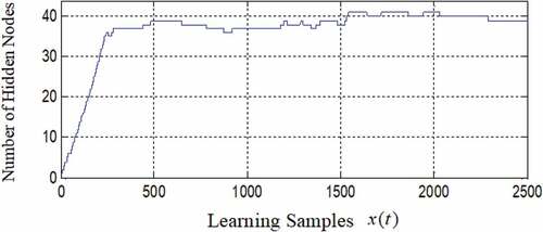
In Figure 4, at the beginning of learning, the training error is large, but it is suppressed quickly by adding hidden nodes. It shows that OSA-RBFNN models the actual output well. Figure 5 shows the training RMSE is large at the beginning of learning and it has a small fluctuation when constructing the network, but the overall trend tends to converge. Figure 6 presents that when t is equal to 241, the hidden nodes reach 36, which completes the construction of the network by adding nodes. In the whole process of learning, the maximum number of hidden nodes reach 41, and the nodes reaches 39 at the end of the training.

Figure 4. The performance of online learning.

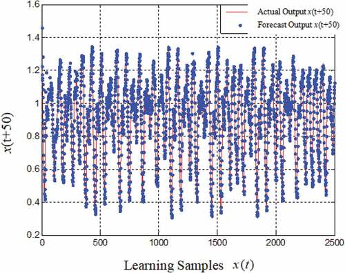
Figure 5. The performance of RMSE.

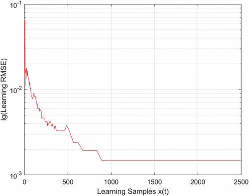
Figure 6. The change in hidden nodes.

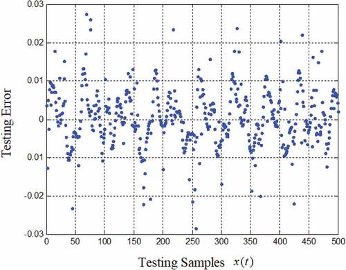
In Figure 7, the maximum error is within 0.03, and the average error of 500 testing samples is 0.0072. For this experiment, we did 20 independent experiments and set the length of the sliding window L equal to 100, 150, and 200, respectively. The results show that the number of hidden nodes was between 39 and 45, and the average error of 500 testing samples was also 0.0072 ~ 0.0136, which is a stable result.

Figure 7. The testing error of 500 samples.

To further verify the effectiveness of the proposed method, we compare OSA-RBFNN with RAN and MRAN. Table 3 indicates that the training RMSE and testing error of OSA-RBFNN on the MG series is lower than the other algorithms.

Table 3. The performance of comparison of different algorithms.

Algorithms	Number of Hidden Nodes	Training RMSE	Testing Error
eTS	99	-^a	-^a
RAN	51	0.0316	0.0427
MRAN	47	0.0274	0.0319
OSAMNN	35	0.0319	-^a
OSA-RBFNN	39	0.0057	0.0072

Note: “^a”Results not listed in the original paper.

The reasons are that we combine the advantages of RAN and MRAN. RAN can modify the parameters of the node when adding a new one; thus, it will improve the learning speed, but the node cannot be pruned once it is added to the RBF network. MRAN can prune inactive hidden nodes to decrease the redundant hidden nodes of the RBF network. We also choose the LM algorithm to estimate the learning rate of each gradient under the curved error surface according to the Hessian matrix. Thus, the learning ability of the RBF network will be improved compared to RAN and RAN. Moreover, we employ a sliding window method to use the latest sample to adjust parameters, it can enhance the accuracy of learning and make the network more stable.

eTS (Rong, Sundararejan, Huang, and Saratchandran Rong et al. 2006)

OSAMNN (Qiao, Zhang, and Bo 2012)

Conclusion

Aiming at the deficiencies that the LM algorithm can not train online RBF network, we propose OSA-RBFNN based on the LM algorithm. We combine the sliding window method with the LM algorithm to build an online self-adaptive network. We also adopt the operations of adding, pruning, and merging hidden nodes to optimize the RBF network structure. Moreover, the hidden nodes are directly added to the training sample with the maximum training error, which can effectively suppress the training error of the current network and avoid adding hidden nodes randomly. Pruning and merging hidden nodes can reduce the impact on the RBF network performance and simplify the network structure. Finally, we have simulation analyze on non-linear function approximation and non-linear time-varying system identification, the results demonstrate that the proposed OSA-RBFNN realizes online modeling with a compact and stable structure. It has a generalization ability with a minimal structure.

Code Availability

Sample code is available on Github (https://github.com/YLiu000222/OSARBFNN)

Disclosure statement

No potential conflict of interest was reported by the author(s).

Additional information

Funding

This work is supported by the [Basic Research plan of Natural Science Foundation of Shaanxi Coal Joint Fund] under Grant [No.2019JLZ-08]; [Basic Research Plan of Nature Science in Shaanxi Province of China] under Grant [No.2020JM-522].

References

- Arif, J., N. Ray Chaudhuri, S. Ray, et al. 2009. Online Levenberg-Marquardt algorithm for neural network based estimation and control of power systems. 2009 International Joint Conference on Neural Networks. Atlanta, GA, USA, 199–3809. IEEE.
- Atif, S. M., S. Khan, I. Naseem, R. Togneri, and M. Bennamoun. 2022. Multi-kernel fusion for RBF neural networks. Neural Processing Letters. doi:10.1007/s11063-022-10925-3.
- Gao, X. 2022. A nonlinear prediction model for Chinese speech signal based on RBF neural network. Multimedia Tools and Applications 81:5033–49. doi:10.1007/s11042-021-11612-6.
- Gu, L., D. K. S. Tok, and D.L. Yu. 2018. Development of adaptive p-step RBF network model with recursive orthogonal least squares training. Neural Compution and Applications 29 (5):1445–54. doi:10.1007/s00521-016-2669-x.
- Hao, Y., P. D. Reiner, T. Xie, T. Bartczak, and B. M. Wilamowski. 2014. An incremental design of radial basis function networks. IEEE Transactions on Neural Networks and Learning Systems 25 (10):1793–803. doi:10.1109/TNNLS.2013.2295813.
- Harpham, C., and C. W. Dawson. 2006. The effect of different basis functions on a radial basis function network for time series prediction: A comparative study. Neurocomputing 69 (16–18):2161–70. doi:10.1016/j.neucom.2005.07.010.
- Houcine Bergou, E., Y. Diouane, and V. Kungurtsev. 2020. Convergence and complexity analysis of a Levenberg–Marquardt algorithm for inverse problems. Journal of Optimization Theory and Applications 185 (3):1–18. doi:10.1007/s10957-020-01666-1.
- Jia, L., W. Li, and J. Qiao. 2022. An online adjusting RBF neural network for nonlinear system modeling. Application Intelligence. Advanced online publication. doi: 10.1007/s10489-021-03106-7.
- Jiang, Q., L. Zhu, C. Shu, and V. Sekar. 2022. An efficient multilayer RBF neural network and its application to regression problems. Neural Computing & Applications 34 (6):4133–50. doi:10.1007/s00521-021-06373-0.
- Kadakadiyavar, S., N. Ramrao, and M. K. Singh. 2020. Efficient mixture control chart pattern recognition using adaptive RBF neural network. International Journal of Information Technology 12 (4):1271–80. doi:10.1007/s41870-019-00381-z.
- Khan, S., I. Naseem, R. Togneri, and M. Bennamoun. 2017. A novel adaptive kernel for the RBF neural networks. Circuits Systems and Signal Processing 36 (4):1639–53. doi:10.1007/s00034-016-0375-7.
- La Rosa Centeno, L., F. C. C. De Castro, M. C. F. De Castro, C. Müller, and S. M. Ribeiro. 2018. Cognitive radio signal classification based on subspace decomposition and RBF neural networks. Wireless Networks 24 (3):821–31. doi:10.1007/s11276-016-1376-y.
- Li, S., Q. Chen, and G.-B. Huang. 2006. Dynamic temperature modeling of continuous annealing furnace using GGAP-RBF neural network. Neurocomputing 69 (4–6):523–36. doi:10.1016/j.neucom.2005.01.008.
- Lu, Y. W., N. Sundararajan, and P. Saratchandran. 1997. A sequential learning scheme for function approximation using minimal radial basis function neural networks. Neural computation 9 (2):461–78. doi:10.1162/neco.1997.9.2.461.
- Meng, X., Y. Zhang, and J. Qiao. 2021. An adaptive task-oriented RBF network for key water quality parameters prediction in wastewater treatment process. Neural Computing & Applications 33 (17):11401–14. doi:10.1007/s00521-020-05659-z.
- Pedro, M. F., and A. E. Ruano. 2009. Online sliding-window methods for process model adaptation. IEEE Transactions Instrumentation and Measurement 58 (9):3012–20. doi:10.1109/TIM.2009.2016818.
- Platt, J. 1991. A resource-allocating network for function interpolation. Neural computation 3 (2):213–25. doi:10.1162/neco.1991.3.2.213.
- Qiao, J., Z. Zhang, and Y. Bo. 2012. An online self-adaptive modular neural network for time-varying systems. Neurocomputing 125:7–16. doi:10.1016/j.neucom.2012.09.038.
- Rong, H.-J., N. Sundararajan, G.-B. Huang, and P. Saratchandran. 2006. Sequential adaptive fuzzy inference system (SAFIS) for nonlinear system identification and prediction. Fuzzy Sets Systems 157 (9):1260–75. doi:10.1016/j.fss.2005.12.011.
- Wilamowski, B. M., and H. Yu. 2010. Improved computation for Levenberg-Marquardt training. IEEE Transactions on Neural Networks 21 (6):930–37. doi:10.1109/TNN.2010.2045657.
- Xi, M., P. Rozycki, J.-F. Qiao, and B. M. Wilamowski. 2018. Nonlinear system modeling using RBF networks for industrial application. IEEE Transactions on Industrial Informatics 14 (3):931–40. doi:10.1109/TII.2017.2734686.
- Yingwei, L., N. Sundararajan, and P. Saratchandran. 1997. Identification of time-varying nonlinear systems using miniman radial basis function neural networks. IEEE Proceedings-Control Theory Applications 144 (2):202–08. doi:10.1049/ip-cta:19970891.
- Zhang, Y., D. Kim, Y. Zhao, and J. Lee. 2020. PD control of a manipulator with gravity and inertia compensation using an RBF neural network. International Journal of Control, Automation, and Systems 18 (12):3083–92. doi:10.1007/s12555-019-0482-x.
- Zhou, K., S.K. Oh, and J. Qiu. 2022. Design of ensemble fuzzy-RBF neural networks based on feature extraction and multi-feature fusion for GIS partial discharge recognition and classification. Journal of Electrical Engineering & Technology 17:513–32. doi:10.1007/s42835-021-00941-z.