Prediction of stock return by LSTM neural network

ABSTRACT

The role of the stock market in the whole financial market is indispensable. How to obtain the actual trading income and maximize the interests in the trading process has been a problem studied by scholars and financial practitioners for a long time. Deep learning network can extract features from a large number of original data, which has potential advantages for stock market prediction. Based on the Shanghai and Shenzhen stock markets from 2019 to 2021, we use LSTM models, optimized on in-sample period and tested on out-of-sample period, using rolling window approach. We select the right hyperparameters at the beginning of our tests, use RBM preprocessing data, then use LSTM model to obtain expected stock return, to effectively predict future stock market analysis and predictive behavior. Finally, we perform a sensitivity analysis of the main parameters and hyperparameters of the model.

Introduction

For a long time, the prediction of future stock price trend and stock return has been an active research field. All investors and researchers hope to achieve the goal of predicting future stock price trend and stock return (Zhong and Enke 2017). The commonly used stock return prediction methods are roughly divided into: fundamental analysis method and technical analysis method. Fundamental analysis method is the most important analysis method that investors preparing for long-term trading should adopt (Zhu et al. 2008). This method focuses on the internal value of stocks and believes that the return needs time to realize. Investors focus on the future prospects of the investment company, observe the current economic factors and examine the company’s income, debt, cash flow, and growth rate from the perspective of the company’s long-term development, after forecasting and analyzing and buying stocks at the right time, you do not have to spend too much time and energy to care about the real-time trend of stock price. On the contrary, for short-term investors, fundamental analysis indicators are of little significance in daily transactions. They prefer to use moving averages, which are more time sensitive technical indicators to reflect the market faster and help them make decisions in a shorter time. Technical analysis is usually considered as a method of medium and short-term investment (Li et al. 2017).

With the increasing number of high-frequency trading data and the inherent complexity and dynamics of stock market prediction, researchers need to improve the relevant technology of stock market prediction, be able to extract abstract features from the data and identify the hidden relationship. Deep learning can automatically extract features from the original data. In the process of feature selection, it needs the least manual intervention and does not need the professional knowledge of macroeconomic variables and other prediction factors, so it can play a key role in stock market prediction. In addition, the market microstructure noise will lead to temporary market ineffectiveness. Many profit opportunities can be found under high frequency, and it is possible to realize statistical arbitrage. Using high-frequency data can get a large data set, and using deep neural network can overcome the problems of data snooping and over fitting in the process of using data (Bengio 2007). Deep neural network can reveal complex patterns and hidden relationships, analyze different indicators and their interactions, so as to predict market behavior and provide solutions that individual investors can’t deal with effectively.

We evaluate the effect of deep learning as a stock return prediction tool and the potential of applying deep learning to broader financial market prediction. There are great differences in the selection of network structure, activation function, and other model parameters. This paper makes a systematic and comprehensive analysis on the application of deep learning. In particular, using stock return as the input data of deep neural network, the overall ability of LSTM neural network to predict future market behavior is tested.

The results show that the prediction performance of deep learning network depends on environmental factors and user determined factors. LSTM deep neural network is effective and can improve the prediction accuracy of stock return. In addition, we also explain how to construct and evaluate the stock return prediction model based on deep learning, which enriches the research of financial prediction market.

Related Research

The stock market changes rapidly, there are many interference factors, and the periodic data are insufficient. Stock trading is a game process under incomplete information. The single objective supervised learning model is difficult to deal with this kind of sequential decision-making problem. Deep learning is one of the effective ways to solve this kind of problem. Traditional quantitative investment is mostly based on technical indicators, with poor adaptability and short investment life. This research aims to introduce the deep learning model into the application of the financial field. Deep learning can process the massive data in the financial market, enhance the ability of data processing and extracting features from the transaction signals to achieve the purpose of stock return analysis (J, S. Z., et al., 2012). For example, stock trading is a sequential decision-making method, and deep learning is to learn multi-stage behavior strategies (Yeh et al., 2011). This method can determine the best return in a certain state and minimize the transaction cost. Therefore, it has the best practicability in the field of investment.

Because of the great success of deep learning in image classification, natural language processing and various time series problems, people apply deep learning to the field of finance. Deep neural network automatically finds the corresponding representation of low dimension by extracting high-dimensional input data. Its core is to integrate the deviation of responders into the hierarchical neural network structure (Evermann, Rehse, and Fettke 2017). Therefore, deep learning has strong ability of perception and feature extraction. Recurrent neural network has recursive feedback connection between neuron cells to form a directed cycle. It can retain and use the information in past data to help predict future events, and can provide a scheme for the construction of cognitive decision-making system of complex system.

Deep neural network provides good stability, universality, and scalability through big data. As candel et al said, “because it performs quite well on many different problems, deep learning is rapidly becoming the preferred algorithm with the highest prediction accuracy (Baranochnikov et al., 2022).” The deep neural network will first have an input layer to match the feature space, then multiple nonlinear layers, and finally a linear regression or classification layer to match the output space. Each non-output layer of the network includes a bias unit (Tumminello et al., 2010). The output of the whole network will be determined by the weight obtained by connecting neurons and deviation from other neurons (Ballings et al. 2015). Therefore, these weights are adjusted to minimize the error on the labeled training data connecting neurons and deviations with other neurons, and fully determine the output of the whole network; When these weights are adjusted to minimize the error on the training data, learning will occur and minimize the loss function of each training instance. Deep learning structure is a model of hierarchical feature extraction, which usually involves multiple levels of nonlinearity (Kijewski and Ślepaczuk 2020). It can learn the useful representation of original data and show high performance on complex data.

Long-short term memory (LSTM) neural network can connect the current and previous events, and this structural time series design method has high accuracy and only depends on the previous events. Therefore, combining different methods and technologies is the fundamental to improve the accuracy of prediction. The research of scholars at home and abroad has also proved this. Sharang published a study on the application of deep belief network (DBN), which is composed of stacked restricted Boltzmann machines, coupled with multilayer perceptron (MLP), and uses the long-range logarithmic return of stock price to predict the return higher than the median (Sharang and Rao 2015). Xiong applied long-term and short-term memory (LSTM) neural network to model the volatility of S & P 500 index, and used Google stock domestic trend as an index of market volatility for relevant research (Xiong, Nichols, and Shen 2015); Fischer and Krauss successfully applied long-term and short-term memory (LSTM) to financial stock market prediction (Fischer and Krauss 2017). The research data set is synthesized by the S & P 500 index. The S & P 500 index combines the list into a binary matrix to eliminate bias and effectively applies the optimizer called “rmsprop.” We put forward the robust concept of time series prediction. The main advantage of the research is that it adopts the most advanced in deep learning technology to provide financial market prediction. The performance of LSTM neural network is better than traditional DNN and logistic regression algorithms. Their methods show that LSTM neural network is suitable for financial time series prediction tasks different from short-term price trend prediction (Grudniewicz and Ślepaczuk 2021). Therefore, we use the coupling of restricted Boltzmann machine and Long-short term memory (LSTM) neural network, and use the long-range logarithmic return of stock price to predict the return above the median.

Theoretical Model

Deep Learning Framework for Stock Return Prediction

For each stock, we seek a predictor function $f$ in order to predict the stock return at time $t+1,$ $r_{t+1},$ given the features $u_t$ extracted from the available information at time $t$. We assume that $r_{t+1}$ can be decomposed into two parts: the predictable part ${\tilde{r}}_{t+1}$=$f\left(x_t\right)$ and the unpredictable part $\epsilon$,

(1) $r_{t+1}={\tilde{r}}_{t+1}+\epsilon$(1)

$u_t$ represents the linear transformation or nonlinear transformation of the current information, including

(2) $u_t=\mathrm{\varnothing }\left(R_t\right)$(2)

和

(3) ${\tilde{r}}_{t+1}=f\left(\mathrm{\varnothing }\left(R_t\right)\right)$(3)

The original available information is defined as the past return of the sample stock. Suppose there are n stocks in the sample and g lagged returns are selected, $R_t$ has the following form:

(4) $R_t={\left[r_{1,t},\dots ,r_{1,t-g+1},\dots ,r_{n,t}\dots ,r_{n,t-g+1}\right]}^T$(4)

where $r_{i,t}$ represents the past earnings of the $i$th stock in the period $t$. In the following part, we will use deep neural network to construct prediction function $f$and conversion function $\mathrm{\varnothing }$, and how to use different data representation methods to construct conversion function.

Data Representation Method

The performance of machine learning algorithm largely depends on the choice of data representation method (Gurjar et al. 2018). Therefore, converting the original data before input can improve the performance of machine learning task. We use limited Boltzmann machine to process the data (Thawornwong and Enke 2004).

Restricted Boltzmann Machine (RBM)

RBM processes input variables $x$ and output variables $u$, defines a function $E\left(x,u\right)$, and obtains the formula from the joint probability density function of $\mathrm{x}$和$u$ (Hinton 2002):

(5) $p\left(x,u\right)=\frac{exp\left(-E\left(x,u\right)\right)}{Z}$(5)

Where $Z\hspace{0.17em}=\sum _{x,u}\mathrm{e}\mathrm{x}\mathrm{p}\left(-E\left(x,u\right)\right)$ is the partition function. In most cases, $u$ is assumed to be a $m$-dimensional binary variable, $u\in \hspace{0.17em}{\left\{0,1\right\}}^m$.When $x$ is a binary or real-valued variable (Taylor et al. 2006), there is a performance function

(6) $Ex,u=1/2(x-b{)}^T{\mathrm{\Sigma }}^{-1}\left(x-b\right)-c^{T}u-u^{T}W{\mathrm{\Sigma }}^{-1/2}x$(6)

where $\mathrm{\Sigma }$，$Wbc$ are the model parameter. $\mathrm{\Sigma }$ set as identity matrix; This makes machine learning easier and simpler with less performance loss (Selvin et al. 2017). According to equations (5)(5) $p\left(x,u\right)=\frac{exp\left(-E\left(x,u\right)\right)}{Z}$(5) and (6(6) $Ex,u=1/2(x-b{)}^T{\mathrm{\Sigma }}^{-1}\left(x-b\right)-c^{T}u-u^{T}W{\mathrm{\Sigma }}^{-1/2}x$(6) ), the conditional probability distribution is as follows:

(7) $p\left(u_j=1|x\right)=\delta \left(c_j+W_{\left(i,:\right)}x\right),i=1,\dots ,m,$(7)

(8) $p\left(x_i|u\right)=\mu \left(b_i+u_i^T{W}_{\left(:,j\right),}1\right),j=1,\dots ,M,$(8)

where $\delta$ is the sigmoid function, $W\left(i;:\right)$和$W\left(:;j\right)$is the row $i$ and column $j$ of $W$. This RBM is called Gauss Bernoulli restricted Boltzmann machine. Then, the conditional probability distribution is used to represent and reconstruct the input data (Nti, Felix, and Asubam 2020). Given an input data set ${\left\{x^n\right\}}_{n=1}^N$, the maximum log likelihood learning formula is as follows:

(9) $\underset{\theta }{max}[L={\sum }_{n=1}^{N}logp\left(x^n,\theta \right)]$(9)

$\theta$=$\left\{Wbc\right\}$ is a model parameter. Because it is difficult to calculate the partition function, the learning method of comparative difference is usually used to estimate the model parameters.

Deep Neural Network

The neural network establishes the nonlinear relationship between two variables. The specific relationship formula is as follows:

(10) $h_{l+1}=\sigma \left(W{h}_l+b\right)$(10)

Among σ is called activation function, which is used to realize the nonlinear transformation of weighted data. The commonly used choices are logistic sigmoid () and hyperbolic tangent () functions, but it is usually different in different network structures. $W$ is the weight matrix and $b$ is the offset vector.

Weight matrix $w=\left[\begin{array}{cccc}{w}_{11}^1& w_{12}^1& \dots & w_{1n}^1\\ w_{21}^2& w_{22}^2& \dots & w_{2n}^2\\ \dots & \dots & \dots & \dots \\ w_{k1}^f& w_{k2}^f& \dots & w_{kn}^f\end{array}\right],b={\left(b_0,b_1,b_2,\dots ,b_n\right)}^T$

Multilayer neural networks extended by advanced learning methods are usually called deep neural networks. The deep neural network can be expressed by superimposing different levels of features according to the needs of the task, and build a deep structure to identify the patterns and relationships related to the corresponding learning task (Roy et al. 2015). Deep neural network operates the high-dimensional original input data, and uses its ability of automatic feature learning to complete the modeling task. The prediction function $y=f\left(x\right)$is constructed by superimposing the network function in the following order (it is the number of layers of the deep neural network):

(11) $h_1=\sigma \left(w^{1}x+b_1\right)$(11)

(12) $h_1=\sigma \left(w^{2}x+b_1\right)$(12)

(13) $y=\sigma \left(w^l{h}_{L-1}+b_L\right)$(13)

Given the input data set $x^n$ and objective function $y^n$, as well as an error function $\epsilon$. In order to make the output function $y^n$= $f\left(x^n\right)$ and the objective function $T^n$, the weight of each node can be adjusted and the model parameters of the whole network can be optimized, so the total error $\theta$ can be minimized. （$\theta \hspace{0.17em}=\hspace{0.17em}\left\{W_1,\hspace{0.17em}\cdot \hspace{0.17em}\cdot \hspace{0.17em}\cdot \hspace{0.17em},\hspace{0.17em}{W}_L,\hspace{0.17em}{b}_1,\hspace{0.17em}\cdot \hspace{0.17em}\cdot \hspace{0.17em}\cdot \hspace{0.17em},\hspace{0.17em}{b}_L\right\}$）

(14) $\underset{\theta }{min}\left[J={\sum }_{n=1}^N\epsilon \left(y^n,T^n\right)\right]$(14)

Select the appropriate $\epsilon \left(\hspace{0.17em}\right)$, its gradient can be obtained by error back propagation analysis. In this case, the minimization problem in (14) can be solved by the usual gradient descent method. The typical form of objective function is as follows:

(15) $J=1/N{\sum }_{n=1}^N{y}^n-T^n{ }^2+\lambda {\sum }_{l=1}^L{W}_l{ }_2$(15)

Where $||.||$ and $||.||{ }_2$ represent Euclidean norm and matrix norm, respectively, the second item is the added “Regularizer.” In equation (15)(15) $J=1/N{\sum }_{n=1}^N{y}^n-T^n{ }^2+\lambda {\sum }_{l=1}^L{W}_l{ }_2$(15) , the second term is regularized to avoid overfitting, and the coefficient is determined at the same time.

LSTM Neural Network

LSTM is a variant of deep neural network, which has the ability to read and interpret sequential data such as text or time series (Babu and Reddy 2014). LSTM network has the ability to use storage units and gates to maintain its status information. These gates enable these networks to reject irrelevant information in the past, remember important information in the current state, and capture the input of the system at the current time, so as to generate output as the prediction of the next time. The state vector in the LSTM memory unit performs aggregation of the old information received from the forget gate and the latest information received from the input gate. Finally, the output gate generates output from the network in the current time slot. This output can be regarded as the next predicted value calculated by the model. In short, LSTM neural network is a powerful tool in the field of machine learning. It can extract features, dimensions, and improve data classification. It is a machine language with the ability to learn internal representation and solve complex combinatorial problems.

Model Data and Trend Prediction

We construct a deep neural network using stock returns from the stock returns of Shanghai and Shenzhen stock markets in 2019–2021. First, we choose the top 50 stocks with average income ranking, and keep only the stocks which have a price record over the entire sample period (50 stocks are listed in Table 1) (Tsai and Hsiao 2010). The stock return is expressed as $r_t=ln\left(E_t/E_{\left(t-t\right)}\right)$, which $t$ means the time difference of five minutes (Castellano Gomez et al. 2021). Each stock in the sample has 750 trading days and 37,500 five-minute return data. Data preprocessing and processing is in Python 3.8 based on Numpy and Pandas packages, RBM and LSTM are implemented with tensorflow. In order to evaluate the performance of the model and avoid over fitting in the training process, we used a rolling window approach, the data set is divided into in-sample (training and validation) and into out-of-sample (test), the training set consists of the first 80% of the samples, including 30,000 stock returns, and the validation set consists of the remaining 20%, including 7500 stock returns, the test set uses 3125 stock returns in the next three months to test (Kim and Sayama 2017). After making the predictions, the window was moved ahead, by the number of periods equal to test set and the model was retrained from scratch (Saâdaoui and Messaoud 2020). Model checkpoint callback function was used to store the best weights (parameters) of the model, based on the lowest loss function value from all trained epochs. These weights were then used for prediction on the test set data. (Jakub Michan´ ków et al. 2022)

Table 1. The sample stocks. They are chosen from the stock returns of Shanghai and Shenzhen stock markets with average return ranking.

Stock ID	Stock name	Stock ID	Stock name
1	China Mobile	26	HuaFon chemical
2	PetroChina	27	TongKun Co., Ltd
3	COSCO shipping	28	Bank of Chengdu
4	Sinopec Group	29	AnGang Steel Co., Ltd
5	MAOTAI liquor	30	Hualu Hengsheng
6	China Shenhua	31	Shougang Co., Ltd
7	BOE A	32	Lu’an green energy
8	WanHua chemical	33	TBEA
9	Baosteel	34	Baofeng energy
10	Citic securities	35	GAC group
11	YanKuang energy	36	ZTE
12	Zijin mining	37	Focus Media
13	ShangGang group	38	Longyuan Power
14	NingDe	39	Erdos resources
15	RongSheng petrochemical	40	COSCO shipping
16	Tianshan Co., Ltd	41	TISCO stainless steel
17	China Coal Energy	42	China Jushi
18	TCL Technology	43	Satellite chemistry
19	Zhifei biology	44	Kangmei
20	Valin steel	45	Daqu energy
21	CDF	46	Gorge energy
22	GuoSen Securities	47	XCMG
23	HoShine silicon	48	Fenjiu group
24	East money	49	Jiangxi Copper
25	TongWei Co., Ltd	50	Baowu

6-China Shenhua energy Co., Ltd., 7-BOE Technology Group Co., Ltd., 8-Wanhua chemical Group Co., Ltd., 9-Baoshan Iron&Steel Co., Ltd., 10-Citic securities Co., Ltd., 11-Yankuang energy Co., Ltd., 12- Zijin mining Group Co., Ltd., 13-Shanghai international port Co., Ltd., 14-Ningde times new energy technology Co., Ltd., 15-Rongsheng petrochemical Co., Ltd., 16-Xinjiang Tianshan cement Co., Ltd., 17- China Coal Energy Co., Ltd., 18- TCL Technology Group Co., Ltd., 19-Chongqing Zhifei biological products Co., Ltd., 20-Hunan Valin Iron&Steel Group Co., Ltd., 21-China Duty Free Group, 22-Guosen Securities Co., Ltd., 23-Hoshine Silicon Industry Co., Ltd., 24-East money information Co., Ltd., 26-Huafon Chemical Co., Ltd., 30-ShanDong Hualu Hengsheng Chemical Co., Ltd., 31-Beijing Shougang co., ltd., 32-Shanxi Lu’an Environmental Protection Energy Development Co., Ltd., 33-TBEA Co., Ltd., 34-Ningxia Baofeng Energy Group Co., Ltd., 35-Guangzhou Automobile Group Co., Ltd., 36-ZTE Communication Co., Ltd., 38-China Longyuan power group Co., Ltd., 39-Inner Mongolia Ordos Resources Co., Ltd., 40-COSCO Shipping Development Co., Ltd., 41-Shanxi Taigang Stainless Steel Co., Ltd., 42-China Jushi Co., Ltd., 43-Satellite Chemical Co., Ltd., 44-Kangmei Pharmaceutical Co., Ltd., 45-Xinjiang Daqu new energy Co., Ltd., 46-China three gorges renewables(group) Co., Ltd., 47-Xuzhou Construction Machinery Group Co., Ltd., 48- Shanxi Xinghuacun Fenjiu Group Co., Ltd., 49-Jiangxi copper Co., Ltd., 50-Magang holding Co., Ltd.

Training set: ${\left\{r_t^n,r_{i,t+1}^n\right\}}_{n=1}^{N_1}$, Test set: ${\left\{r_t^n,r_{i,t+1}^n\right\}}_{n=1}^{N_2},i=1,\dots ,M.$

All stock returns are standardized by using the mean ${\mu }_i$ and standard deviation ${\sigma }_i$ of the training set (Wang et al., 2011). The standardized rate of return is: $\frac{r_{i,t}-{\mu }_i}{{\sigma }_i}$, and 10 lagged returns of stocks in the sample are used as data input each time:

(16) $R_t={\left[r_{1,t},\dots r_{1,t-9},r_{38,t},r_{38,t-9}\right]}^T$(16)

Evidence of Predictability in the Shanghai and Shenzhen Stock Market

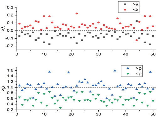
As an example of prediction, we carry out a simple experiment to see whether past returns have predictable power for future returns (Bui and Ślepaczuk 2021). We first divide the returns of each stock into two groups according to the mean or variance of 10 lagged returns: if the mean of lagged returns, $M\left(10\right)$, is greater than a certain threshold λ, the return is assigned to one group; otherwise, it is assigned to the other group. Similarly, by comparing the variance of lagging returns, $V\left(10\right)$, with a threshold ρ, the returns are divided into two groups.

The classification is carried out in the training set, and the threshold λ and ρ are chosen for each stock so that the two groups have the same size (Rundo 2019). These thresholds are then applied to the test set to classify the returns, and the mean and variance of each group are calculated (Yoshihara et al. 2014).

The results are shown in Table 2 and Figure 1. It is clear from the first chart that the average rate of return $M\left(10\right)$ > λ. The prices of all stocks except 44 are lower than those of the other group. Obviously, the average difference between the two groups is significant for all stocks at a 99% confidence interval. Under the 99% confidence interval, the variance difference of all stocks is significant. This shows that the past returns do have a certain prediction ability, which can further use deep feature learning (Zhang et al. 2021).

Table 2. Mean and variance of stock returns of each group in the test set. The second and the third columns are mean returns of each group and the fourth column is the p-value of t-test on the mean difference. The last three columns are variances of the returns and the p-value of F-test on the variance difference.

Stock ID	$M\left(10\right)$>λ	$M\left(10\right)$<λ	$p$	$V\left(10\right)$>ρ	$V\left(10\right)$< ρ	$p$
1	−0.072	0.091	0.000	1.060	0.652	0.000
2	−0.021	0.029	0.000	0.895	0.379	0.000
3	−0.050	0.049	0.000	0.960	0.559	0.000
4	−0.039	0.054	0.000	1.109	0.543	0.000
5	−0.072	0.068	0.000	1.070	0.612	0.000
6	−0.023	0.033	0.000	0.626	0.353	0.000
7	−0.123	0.122	0.000	0.934	0.567	0.000
8	−0.098	0.113	0.000	1.116	0.802	0.000
9	−0.042	0.010	0.000	1.017	0.465	0.000
10	−0.153	0.187	0.000	1.142	0.769	0.000
11	−0.047	0.034	0.000	0.949	0.360	0.000
12	−0.177	0.186	0.000	1.550	0.840	0.000
13	−0.094	0.107	0.000	1.006	0.627	0.000
14	−0.007	0.041	0.000	0.693	0.426	0.000
15	−0.064	0.044	0.000	1.109	0.538	0.000
16	−0.043	0.023	0.000	0.728	0.275	0.000
17	−0.067	0.082	0.000	0.989	0.638	0.000
18	−0.069	0.072	0.000	1.025	0.547	0.000
19	−0.028	0.021	0.000	1.528	0.643	0.000
20	−0.091	0.054	0.000	0.989	0.656	0.000
21	−0.089	0.040	0.000	0.879	0.558	0.000
22	−0.165	0.223	0.000	1.056	0.828	0.000
23	−0.043	0.047	0.000	1.202	0.523	0.000
24	−0.125	0.083	0.000	1.177	0.834	0.000
25	−0.066	0.071	0.000	1.278	0.542	0.000
26	−0.023	0.039	0.000	1.168	0.562	0.000
27	−0.026	0.063	0.000	0.846	0.528	0.000
28	−0.080	0.090	0.000	1.066	0.744	0.000
29	−0.065	0.038	0.000	1.067	0.601	0.000
30	−0.095	0.107	0.000	1.137	0.729	0.000
31	−0.037	0.021	0.000	1.209	0.527	0.000
32	−0.086	0.073	0.000	1.068	0.486	0.000
33	−0.048	0.047	0.000	0.607	0.355	0.000
34	−0.009	0.031	0.001	0.946	0.547	0.000
35	−0.067	0.028	0.000	0.731	0.457	0.000
36	−0.020	0.018	0.000	1.594	0.575	0.000
37	−0.113	0.160	0.000	1.028	0.542	0.000
38	−0.079	0.095	0.000	1.069	0.657	0.000
39	−0.023	0.035	0.000	0.915	0.385	0.000
40	−0.049	0.053	0.000	0.956	0.560	0.000
41	−0.038	0.053	0.000	1.113	0.556	0.000
42	−0.073	0.076	0.000	1.071	0.613	0.000
43	−0.024	0.034	0.000	0.627	0.351	0.000
44	0.124	−0.124	0.032	0.935	0.564	0.000
45	−0.099	0.114	0.000	1.117	0.803	0.000
46	−0.041	0.009	0.000	1.018	0.467	0.000
47	−0.154	0.188	0.000	1.141	0.771	0.000
48	−0.048	0.035	0.000	0.953	0.359	0.000
49	−0.178	0.187	0.000	1.548	0.838	0.000
50	−0.069	0.056	0.000	0.942	0.521	0.000

Figure 1. Mean and variance of stock returns of each group in the test set. The figure above shows the average return of each group of stocks defined by the average value of past return. The following figure shows the variance of each group of returns defined by the variance of past returns. The x-axis represents the stock serial number.

Market Representation and Trend Prediction

Restricted Boltzmann machine (RBM) is used to receive the original feature input and generate the output, $u_t=\mathrm{\varnothing }\left(R_t\right)$. Figure 2 and Table 3 show the prediction accuracy and reference accuracy of each data set through RBM.

Figure 2. Upper figure: prediction accuracy and reference accuracy of each data set. Figure below: difference between test set precision.

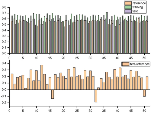
Table 3. Up/Down prediction accuracy of RBM.

	$\mathrm{e}\mathrm{r}\mathrm{r}\mathrm{o}\mathrm{r}\frac{1}{n}\sum _{n=1}^N||x^n-x{ }_{rec}^n|{|}^2$		Up and down prediction accuracy
	Training set	Test set	Training set	Test set
RBM	75.3	66.05	0.661	0.609

Then, according to the prediction function ${\tilde{r}}_{t+1}$=$f\left(u_t\right)$, the LSTM neural network is used to predict its performance (Nguyen and Ślepaczuk 2022), and compared with the univariate autoregressive model (AR (10)) with 10 lag returns. Input variable: price/return ratio (PE); Price/dividend ratio (PD); Period difference (TMS); Default spread (dfy); Lagging stock return (R). Output variable: stock return forecast (Thawornwong and Enke 2004). Through the RBM input variables, the LSTM network is trained by minimizing the objective function defined in equation (15)(15) $J=1/N{\sum }_{n=1}^N{y}^n-T^n{ }^2+\lambda {\sum }_{l=1}^L{W}_l{ }_2$(15) through 3000 learning iterations, and the 3125 stock returns in the next three months are used as the verification set stopped in advance to avoid overfitting (Chai, Draxler, and Stein 2015).(As shown in Figure 3)

Figure 3. Data processing flow chart.

Hyperparameters Turning

During our research, we conducted detailed hyperparameters tuning to ensure the best possible results from our model (Michańków et al. 2022). During the process, we optimized the following parameters:

The number of layers (5) and neurons in each layer (512/256/128).

Dropout rate (0.02) and L2 kernel regularization (0.0005).

The optimizer (Adam variants).

Learning rates (0.005) and momentum values (0.5).

As for the input data, we tuned the training and testing/rolling window sizes, sequence length (2–20), batch size (from 16 to test size) and training process duration, which was set by the number of epochs (10–300), as well as callback functions of early stopping and model checkpoint. Only the first window of data was used for tuning, and the best hyperparameters were then used for the remaining iteration during the walk forward predictions.

Most of the tuning was done using the Tensorflow framework, we could test how changes to several parameters at once would affect the network performance, instead of testing each hyperparameter separately (Srivastava et al. 2014). In addition, we also conducted a careful manual sensitivity analysis on the parameters that had the most impact on the results. (Jakub Michan´ ków et al. 2022)

Performance Evaluation

We evaluate the prediction performance using four measures: normalized mean squared error (NMSE), root mean squared error (RMSE), mean absolute error (MAE), and mean absolute directional loss (MADL). (Jakub Michan´ ków et al. 2022)

Normalized Mean Squared Error

Given a set of target returns and their predicted values, ${\left\{r_{t+1}^n,{\tilde{r}}_{t+1}^n\right\}}_{n=1}^N$, NMSE formula is as follows:

NMSE=$\frac{1}{N}\frac{{\sum }_{n=1}^N{\left(r_{t+1}^n-{\tilde{r}}_{t+1}^n\right)}^2}{var\left(r_{t+1}^n\right)}$

Where var () represents variance and NMSE is the minimum MSE normalization obtained from constant prediction.

Root Mean Square Error

RMSE is the square root of MSE. The RMSE formula is as follows:

RMSE=$\sqrt{\frac{1}{N}}{\sum }_{N=1}^N{\left(r_{t+1}^n-{\tilde{r}}_{t+1}^n\right)}^2$

Mean Absolute Error

MAE is calculated as follows:

$\mathrm{M}\mathrm{A}\mathrm{E}=\frac{1}{\mathrm{N}}{\sum }_{\mathrm{n}=1}^{\mathrm{N}}\left|{\mathrm{r}}_{\mathrm{t}+1}^{\mathrm{n}}-{\tilde{\mathrm{r}}}_{\mathrm{t}+1}^{\mathrm{n}}\right|$

The inequality is applicable to the measurement of RMSE and NMSE, and their size relationship; MAE≤RMSE≤NMAE; Although Mae gives the same weight to all error quantities, RMSE is more sensitive to outliers and more suitable for normal distribution errors (Chai, Draxler, and Stein 2015).

Mean Absolute Directional Loss (MADL)

In order to improve the usefulness of forecasting ability of LSTM model in algorithmic investment strategies (AIS), we adopted Jakub Michan´ ków et al.’s Mean Absolute Directional Loss (MADL) that can be calculated using the following formula:

$MADL=\frac{1}{N}\sum _{t=1}^N\left(-1\right)sign\left(r_{t+1}^n-{\tilde{r}}_{t+1}^n\right)abs\left(r_{t+1}^n\right)$

where: MADL is the Mean Absolute Directional Loss, $r_{t+1}$is the observed return on interval $t+1$, ${\tilde{r}}_{t+1}$ is the predicted return on interval $t+1$. This way, the value the function returns will be equal to the observed return on investment with the predicted direction, which allows the model to tell if the prediction will yield profit or loss and how much this profit or loss will be. The function of MADL is minimized, so that if it returns the negative values the strategy will make a profit, and if it returns a positive value the strategy will generate a loss. MADL was the main loss function used in hyperparameters tuning and in the estimation of the LSTM model.

Prediction Results

We use classic loss function NMSE, RMSE, MAE and MADL loss function, NMSE, RMSE, MSE were used as our starting point in comparing the performance of LSTM networks, we saw that results based on MADL function are much better in prediction.

Table 4 shows the performance of LSTM network in NMSE, RMSE, MSE, MADL, MADL-AR. MADL is more accurate than classic loss function prediction. We combine LSTM with AR (10) to enhance predictability. When LSTM is applied to the residuals of AR (10), MADL increases slightly, with little effect, but the characteristics are consistent. Regardless of the feature selection, LSTM improves prediction performance for all representations.

Table 4. Performance of LSTM network in NMSE, RMSE, MSE, MADL, MADL -AR.

Stock ID	NMSE	RMSE	MAE	MADL	MADL-AR
1	0.9401	0.9640	0.6402	0.9557	0.9522
2	0.9453	1.0052	0.4867	0.9869	0.9082
3	0.9479	0.9755	0.5855	0.9638	0.9311
4	0.9304	0.9832	0.6018	0.9555	0.9534
5	0.9546	0.9809	0.6192	0.9505	0.9741
6	0.9490	0.9821	0.4201	0.9558	0.9589
7	0.9122	0.9404	0.5737	0.9161	0.9233
8	0.9228	0.9609	0.7025	0.9547	0.9597
9	0.9661	0.9978	0.5360	0.9948	1.0006
10	0.8699	0.8969	0.6900	0.8823	0.8800
11	0.9458	0.9824	0.4358	0.9817	0.9950
12	0.9165	0.9123	0.7725	0.9190	0.9015
13	0.9143	0.9572	0.6350	0.9413	0.9494
14	0.9676	1.0061	0.4816	0.9919	1.0043
15	0.9487	0.9725	0.5873	0.9647	0.9608
16	0.9621	0.9922	0.3745	0.9987	1.0067
17	0.9269	0.9547	0.6311	0.9551	0.9512
18	0.9297	0.9762	0.5863	0.9647	0.9738
19	0.9444	1.0099	0.6552	1.0408	1.0377
20	0.9160	0.9566	0.6087	0.9650	0.9663
21	0.9683	0.9768	0.5683	0.9670	0.9697
22	0.7832	0.8932	0.7114	0.8692	0.8932
23	0.9570	0.9914	0.5947	0.9888	0.9355
24	0.9432	0.9488	0.7371	0.9461	0.9423
25	0.9612	0.9810	0.5984	0.9704	0.9743
26	0.9664	0.9807	0.6237	0.9750	0.9738
27	0.9463	0.9858	0.5641	0.9741	0.9820
28	0.8856	0.9711	0.6940	0.9537	0.9731
29	0.9573	0.9821	0.5968	0.9211	0.9233
30	0.9244	0.9595	0.6867	0.9493	0.9575
31	0.9551	0.9753	0.6033	0.9713	0.9682
32	0.9558	0.9758	0.5830	0.9566	0.9626
33	0.9462	0.9749	0.4303	0.9612	0.9675
34	0.9223	0.9897	0.5706	0.9242	0.9986
35	0.9548	0.9847	0.5162	0.9665	0.9768
36	0.9693	1.0039	0.6666	1.0109	1.0124
37	0.8429	0.9125	0.5913	0.8887	0.9021
38	0.9406	0.9741	0.5633	0.9443	0.9187
39	0.9904	0.9732	0.7068	0.9685	0.8724
40	0.9452	0.9786	0.5937	0.9357	0.9894
41	0.9780	0.9028	0.7329	0.9243	0.9443
42	0.9815	0.9418	0.5951	0.9548	0.9685
43	0.9866	0.9996	0.6188	0.9195	0.9757
44	0.9716	0.9602	0.5653	0.9495	0.9243
45	0.9795	0.9859	0.6921	0.9655	0.9548
46	0.9596	0.9546	0.5933	0.9542	0.9795
47	0.9667	0.9611	0.6838	0.9227	0.9495
48	0.9630	1.0074	0.6029	0.9358	0.9255
49	0.9670	0.9529	0.5805	0.9658	0.9542
50	0.9937	0.9790	0.4270	0.9443	0.9627
average	0.9434	0.9693	0.5983	0.9544	0.9564

Sensitivity

We compute the gradient of each predictor function with respect to the input features to identify the contribution of each feature to the prediction (Cakra and Trisedya 2016). We compute a sensitivity matrix $S\in R^{M\times Mg}$from the test set as follows:

$S_{ij}=\frac{1}{N_2}\sum _{n=1}^{N_2}\left|J_{ij}^n\right|$

where $J_{ij}^n$ is $J_{ij}$ of the $n$th data in the test set. The sensitivities are visualized in Figure 4. White color represents zero sensitivity and a darker color means a higher sensitivity. It is interesting to note that, for LSTM, the sensitivity of $f_i$ is particularly high with respect to $u_{j,t}$ for $j=i,i+M$, and $i+2M$.

Figure 4. Heat map of the sensitivity matrix. This represents the sensitivity of the predictor functions with respect to the past returns. y-axis represents the prediction function of each stock return, and x-axis represents the past returns of the stocks in the order of $r_{1,t}$, $r_{2,t}$, … … , $r_{1,t-1}$, $r_{2,t-1}$, … … , $r_{50,t-4}$. Sensitivities to the lagged returns with lag > 5 are omitted as their values are close to 0. White represents zero sensitivity and darker color means higher sensitivity.

Conclusion

Our research suggest that the stock returns are predictable to some extent, a stock market prediction model based on deep feature learning is proposed. From the original level input composed of lagging stock returns, the data are represented by restricted Boltzmann machine, and the LSTM neural network is constructed to predict the future stock returns. The results show that LSTM performs better than linear autoregressive model in the test set. The prediction of stock return is mainly affected by the lag return. By applying LSTM to the residual of autoregressive model, it is found that LSTM can extract additional information and improve the prediction. These research results can help high-frequency traders improve stock returns, predict overall market returns and risks, and can also be used in the trading market of index derivatives such as index futures and options.

One of the main advantages of LSTM neural network is that it can extract features from a large number of original data without relying on the prior knowledge of predictors. This makes deep learning especially suitable for stock market prediction. In stock market prediction, many factors affect stock prices in complex and nonlinear ways. If there are factors with predictable evidence, these factors can be used as part of the input data of in-depth learning to determine the relationship between these factors and stock price.

As one of the studies to test the effectiveness of deep feature learning in stock market analysis and prediction, we provide a direction for the expansion and further research of the advantages of deep learning network. The combination of limited Boltzmann machine and LSTM network function can provide better performance. In addition, the equity risk premium needs to be considered in future research. It is also noted that when the training set is too refined, the risk of overfitting will increase.

Acknowledgments

The work is supported by the following project grants, National Social Science Foundation funded project Research on vulnerability diagnosis and ‘data governance’ model of urban drainage system（17BGL210）; Tianjin’s key soft science research project Research on Countermeasures to vigorously promote global science popularization in Tianjin（19ZLZDZF00270）.

Disclosure statement

The authors declare that they have no known competing financial interests or personal relationships that could have appeared to influence the work reported in this paper.

Data Availability Statement

All employed data will be made available on reasonable request. http://data.cnstock.com/

Additional information

Funding

This work was supported by National Social Science Foundation funded project Research on vulnerability diagnosis and ‘data governance’ model of urban drainage system（17BGL210）; Tianjin’s key soft science research project Research on Countermeasures to vigorously promote global science popularization in Tianjin（19ZLZDZF00270）.

References

- Babu, C. N., and B. E. Reddy. 2014. A moving-average filter based hybrid ARIMA–ANN model for forecasting time series data. Applied Soft Computing 23 (Complete):27–3927. doi:10.1016/j.asoc.2014.05.028.
- Ballings, M., V. Dirk, N. Hespeels, and R. Gryp. 2015. Evaluating multiple classifiers for stock price direction prediction. Expert Systems with Applications 42 (20):7046–56. doi:10.1016/j.eswa.2015.05.013.
- Baranochnikov, I. Ś. R., 2022, A comparison of LSTM and GRU architectures with the novel walk-forward approach to algorithmic investment strategy, Working papers of faculty of economic sciences, University of Warsaw, WP 21/2022 (397), https://www.wne.uw.edu.pl/application/files/3516/5945/4534/WNE_WP397.pdf.
- Bengio, Y. 2007. Scaling learning algorithms towards ai. Large Scale Kernel Machines 34 (5):1–41. doi:10.1016/j.asoc.2014.05.028.
- Bui, Q., and R. Ślepaczuk. 2021. Applying hurst exponent in pair trading strategies on nasdaq 100 index. Physica A: Statistical Mechanics and Its Applications 592:126784. https://www.sciencedirect.com/science/article/abs/pii/S037843712100964X.
- Cakra, Y. E., and B. D. Trisedya. Stock price prediction using linear regression based on sentiment analysis. International Conference on Advanced Computer Science & Information Systems USA, IEEE, 2016.
- Carreira-Perpinan, M. A., and G. E. Hinton 2005. On contrastive divergence learning. proceedings of artificial intelligence & statistics R5: 33–40 . .
- Castellano Gomez, S., and R. Ślepaczuk, 2021, Robust optimization in algorithmic investment strategies, Working papers of faculty of economic sciences, University of Warsaw, WP 27/2021 (375), https://www.wne.uw.edu.pl/application/files/8616/3847/9793/WNE_WP375.pdf.
- Chai, T., R. Draxler, and A. Stein. 2015. Source term estimation using air concentration measurements and a lagrangian dispersion model – experiments with pseudo and real cesium-137 observations from the fukushima nuclear accident. Atmospheric Environment 106 (apr):241–51. doi:10.1016/j.atmosenv.2015.01.070.
- Evermann, J., J. R. Rehse, and P. Fettke. 2017. Predicting process behaviour using deep learning. Decision Support Systems 100:129–40. doi:10.1016/j.dss.2017.04.003.
- Fischer, T., and C. Krauss. 2017. Deep learning with long short-term memory networks for financial market predictions. European Journal of Operational Research 270 (2):654–69. doi:10.1016/j.ejor.2017.11.054.
- Grudniewicz, J., and R. Ślepaczuk, 2021, Application of machine learning in quantitative investment strategies on global stock markets, Working Papers of faculty of economic sciences, University of Warsaw, WP 23/2021 (371), https://www.wne.uw.edu.pl/files/6216/3603/4435/WNE_WP371.pdf.
- Gurjar, M., P. Naik, G. Mujumdar, and T. Vaidya. 2018. Stock market prediction using ann. International Research Journal of Engineering and Technology 5 (3):2758–61.
- Hinton, G. E. 2002. Training products of experts by minimizing contrastive divergence. Neural Computation, págs1771–1800. doi: 10.1162/089976602760128018.
- J, S. Z. et al. 2012. A review of research on deep learning. Computer Application Research 29 (8):2806–10. doi:10.48550/arXiv.1206.5538.
- Kijewski, M., and R. Ślepaczuk, 2020, Predicting prices of S&P500 index using classical methods and recurrent neural networks, Working papers of faculty of economic sciences, University of Warsaw, WP 27/2020 (333), https://www.wne.uw.edu.pl/application/files/4616/3609/7114/WNE_WP333.pdf.
- Kim, M., and H. Sayama. 2017. Predicting stock market movements using network science: An information theoretic approach. Applied Network Science 2 (1):35. doi:10.1007/s41109-017-0055-y.
- Li, Z. B., G. Y. Yang, Y. C. Feng, and L. Jing. 2017. Empirical test of Fama French five factor model in China’s stock market. Financial Research 6:191–206.
- Michańków, J., P. Sakowski, and R. Ślepaczuk. 2022. The comparison of LSTM in algorithmic investment strategies on BTC and SP500 index. Sensors 22:917. doi:10.3390/s22030917.
- Nguyen, V., and R. Ślepaczuk. 2022. Applying hybrid ARIMA-SGARCH in algorithmic investment strategies on S&P500 Index. Entropy 24 (2):158. doi:10.3390/e24020158.
- Nti, I. K., A. A. Felix, and W. B. Asubam. 2020. A systematic review of fundamental and technical analysis of stock market predictions. Artificial Intelligence Review 53 (4):3007–57. doi:10.1007/s10462-019-09754-z.
- Qiu, M., Y. Song, and F. Akagi. 2016. Application of artificial neural network for the prediction of stock market returns: The case of the japanese stock market. Chaos Solitons & Fractals the Interdisciplinary Journal of Nonlinear Science & Nonequilibrium & Complex Phenomena 85:1–7. doi:10.1016/j.chaos.2016.01.004.
- Roy, S. S., D. Mittal, A. Basu, and A. Abraham. 2015. Stock market forecasting using lasso linear regression model. Springer International Publishing. doi:10.1007/978-3-319-13572-4_31.
- Rundo. 2019. Deep LSTM with reinforcement learning layer for financial trend prediction in fx high frequency trading systems. Applied Sciences 9 (20):4460. doi:10.3390/app9204460.
- Saâdaoui, F., and O. B. Messaoud. 2020.Multiscaled neural autoregressive distributed lag: A new empirical mode decomposition model for nonlinear time series forecasting. International Journal of Neural Systems 30: 2050039.doi: 10.1142/S0129065720500392
- Selvin, S., R. Vinayakumar, E. Gopalakrishnan, V. K. Menon, and K. Soman (2017). Stock price prediction using lstm, rnn and cnn-sliding window model. In 2017 International Conference on Advances in Computing, Communications and Informatics (ICACCI), USA, pp. 1643–47. IEEE.
- Sharang, A., and C. Rao 2015. Using machine learning for medium frequency derivative portfolio trading. Papers. doi: 10.48550/arXiv.1512.06228.
- Srivastava, N., G. Hinton, A. Krizhevsky, I. Sutskever, and R. Salakhutdinov 2014. Dropout: A simple way to prevent neural networks from overfitting. Journal of Machine Learning Research, 15(1), 1929–58. doi: 10.1016/j.neucom.2015.09.116.
- Taylor, G. W., G. E. Hinton, and S. T. Roweis. 2006. Modeling human motion using binary latent variables. Advances in Neural Information Processing Systems 19, 1345–52.
- Thawornwong, S., and D. Enke. 2004. The adaptive selection of financial and economic variables for use with artificial neural networks. Neurocomputing 56:205–32. doi:10.1016/j.neucom.2003.05.001.
- Ticknor, J. L. 2013. A bayesian regularized artificial neural network for stock market forecasting. Expert Systems with Applications 40 (14):5501–06. doi:10.1016/j.eswa.2013.04.013.
- Tsai, C.-F., and Y.-C. Hsiao. 2010. Combining multiple feature selection methods for stock prediction:Union, intersection, and multi-intersection approaches. Decision Support Systems 50 (1):258–69. doi:10.1016/j.dss.2010.08.028.
- Tumminello, M., F. Lillo, and R. N. Mantegna. 2010. Correlation, hierarchies, and networks in financial markets. Journal of Economic Behavior & Organization 75 (1):40–58. doi:10.1016/j.jebo.2010.01.004.
- Wang, J.-Z., J.-J. Wang, Z.-G. Zhang, and S.-P. Guo. 2011. Forecasting stock indices with back propagation neural network. Expert Systems with Applications 38 (11):14346–55. doi:10.1016/j.eswa.2011.04.222.
- Xiong, R., E. P. Nichols, and Y. Shen. 2015. Deep learning stock volatility with google domestic trends. arXiv preprint arXiv :151204916 2015 .
- Yeh, C.-Y., C.-W. Huang, and S.-J. Lee. 2011. A multiple-kernel support vector regression approach for stock market price forecasting. Expert Systems with Applications 38 (3):2177–86. doi:10.1016/j.eswa.2010.08.004.
- Yoshihara, A., K. Fujikawa, K. Seki, and K. Uehara 2014. Predicting stock market trends by recurrent deep neural networks. In Pacific rim international conference on artificial intelligence. 759–69. doi: 10.1007/978-3-319-13560-1_60.
- Zhang, X., G. Naijie, C. Jie, and Y. Hong. 2021. Predicting stock price movement using a dbn-rnn. Applied Artificial Intelligence 35 (12):876–92. doi:10.1080/08839514.2021.1942520.
- Zhong, X., and D. Enke. 2017. Forecasting daily stock market return using dimensionality reduction. Expert Systems with Applications 67:126–39. doi:10.1016/j.eswa.2016.09.027.
- Zhu, X., H. Wang, L. Xu, and H. Li. 2008. Predicting stock index increments by neural networks: The role of trading volume under different horizons. Expert Systems with Applications 34 (4):3043–54. doi:10.1016/j.eswa.2007.06.023.