An effective tumor detection in MR brain images based on deep CNN approach: i-YOLOV5

ABSTRACT

With the advent of computer technology, Artificial Intelligence (AI) aids radiologists to diagnosis the Brain Tumor (BT). Early detection of diseases can be increased in health care leads to further treatments, wherein the typical application of AI systems performs a vital role in terms of time and money savings. Magnetic Resonance (MR) images are enhanced with image enhancement techniques to improve contrast and color accuracy. Besides, traditional methods uncompensated for problems with the several types of MR imaging for BT. Deep learning techniques can be extended to help overcome the common problems encountered in conventional tumor detection methods. Therefore, in this work, an improvised YOLOV5 technique have been proposed for BT detection based on MR images. Eventually, the idea of Hyperparameter Optimization (HPO) is applied using Hybrid Grid Search Optimizer Algorithm (HGSOA) to enhance the performance of the tumor detection viz tuning of hyper parameters in proposed deep neural network. To evaluate the effectiveness of proposed model, McCulloch’s algorithm is used to localize images for tumor region segmentation, and the segmentation result is also checked with truth annotated images. Various experiments were conducted to measure the accuracy of proposed fine-tuned model using MW brain test images. Finally, classification metrics including, MSE, PSNR, SSIM, FSIM, and CPU time are compared with existing state-of-the-art techniques to prove the effectiveness of the proposed model. In the taxonomy of MRI-BT, greater precision was achieved by CNN.

Introduction

The improvement in people’s standard of living is drastic with fast economic development. Moreover, there is a significant reinforcement of healthcare systems’ proportion and a gradual increase of health awareness camps in societies. There has been an exponential expansion and promotion of healthcare technology in the past few years. The future of healthcare and enhanced public health has been molded by state-of-the-art technologies (Dosovitskiy et al. 2020). For instance, by possessing image processing as a significant component, patients’ healthcare has been improved by successfully applying Computer Vision (CV) technology in medical imaging. It is a great challenge to detect BT in humans as the brain is susceptible organ. Generally, radiologist find difficult to identify the BT from MR images which may consume more time. A second opinion on the existence (or) nonexistence of a tumor happens in the mind of the radiologist with the help of a Computer-Aided Diagnostic (CAD) system, which has to be boosted for effective performance.

BT refers to the aggregation of abnormal cells in some tissues of the brain. Primary and metastatic BT are the two groups that are separated based on the origin of the tumors. Even benign tumors can disable the brain and have permanent repercussions since BT are present in the center of the human neurological system. The accumulation of aberrant cells in some brain areas was referred to as a BT. Primary and metastatic BT are the two groups that are separated based on the origin of the tumors. Even benign tumors can disable the brain and have permanent repercussions since BT are present in the center of the human neurological system. The study of brain images is facilitated by Magnetic Resonance Imaging (MRI) which plays a significant role in research in neuroscience. The prevailing segmentation techniques require a massive amount of precise data that is difficult to obtain in the medical field. Some of the research studies deal with inaccurate data in medical images. Moreover, the modeling of healthy brain distributions at high resolution for detection and delineation, especially of small brain lesions with greater accuracy, has been emphasized in this research work. The goal is to assist radiologists with more targeted and accurate disease detection, like BT using enhanced AI to implement unique tools for analyzing medical images.

Recently, in image classification, significant success has been achieved by Deep Learning (DL) (Dosovitskiy et al. 2021; Mitani et al. 2020), a kind of AI in which the patterns are learned by Neural Networks (NN) directly from raw data. The detection and classification of tumors into glioma, pituitary, and meningioma are done with the help of a technique based on DL. From the segmented images, the features are mined regarding tumor region, texture, color, edge, and location. From the segmented images, the classification techniques are used classifying to obtain a conclusion on whether the patient is having or not having a tumor. The issues confronted in the previous research have been overcome in this paper by introducing YOLOV5.

Nevertheless, high-level training skills are required for skilled engineers. Human beings are prone to making mistakes, even after training for many years. Hence, to a certain extent, DL can mitigate such errors. Hard-to-detect diseases can be verified with the help of programmed machines, especially using DL algorithms. Building a trainable model that can automatically mine the features that belong to particular tasks has been made feasible due to the enhanced DL (Anaraki, Ayati, and Kazemi 2019). When compared to conventional, ML and DL can perform better in various domains, like medical image segmentation. The segmentation of tumors using DL techniques can be time effective for hospitals and patients. Besides, the diagnosis is also very accurate with the application of this technique. This author presents fully-automated CNN models for multi-level classification of BT that have used open-access datasets.

The quality of digital imaging has been projected to be improved by using a different modified Anisotropic Diffusion (AD) models using other methods (Malarvel et al. 2017). The level of noise is reduced by spatial information. A standard method known as linear diffusion is used in spatial information to smooth an image under the control of kernel tricks. The benign and malignant BT that grow at a slow pace are not very hazardous to the human body. As a result, cells and other organs in the body find proof of general and specific cell spread in BT. The result of various Image Quality metrics, MSE, PSNR, SSIM, and FSIM, is achieved by the proposed method compared with the previous research.

Moreover, minimum computation time is taken (Menze et al. 2015). To solve the problem of tumor classification, ML algorithms like Support Vector Machine (SVM), Approximate Nearest Neighbor (ANN), and K-Nearest Neighbor (KNN) are applied in this work. In the taxonomy of MRI-BT, greater precision was achieved by CNN, like the accuracy of 91% obtained by benign/malicious scans (Bahadure, Ray, and Tethi 2017). Moreover, the binary classification systems are assessed by applying this. 90.19% and 91.26% are the CNN accuracy and F1-score, respectively. An i-YOLOV5 object detection model based on DL, which can categorize the abnormalities in the BT, (i.e.,) as benign (or) malignant, and detect their exact location in the rebuilt brain images, is presented in this research. To achieve brilliant accuracy, several techniques of You-Only-Look-Once (YOLO) are applied to researchers. The assessed results explicitly show the less memory size of 22.989 MB possessed by i-YOLOV5. Because of its weird attributes, such as Mosaic data improvement and computation of adaptive anchor frames, among the rest of object detection algorithms YOLOV5 (Bochkovskiy 2020) outperforms its counterparts. The outperformance of i-YOLOV5 is in terms of speed and smaller size, apart from its well-planned architecture.

The overall contribution of the proposed work has been given as follows:

• The proposed deep CNN-based i-YOLOV5 model is extended for classification of benign and malignant tumors. To handle the imbalanced dataset of MR brain images, the idea of Bounding Box (BB) techniques have been extended. It has been fine-tuned to work optimally and run appropriately for most cases with reliable performance. MR brain image testing datasets were used to measure tumor classification and detection ability.

• According to the experimental results, the multi-classification of the brain from the existing MRI images has been tried as preliminary work. It is implemented using CNN for Hyper Parameters Optimization (HPO), which is automatically modified with the support of the Hybrid Grid Search Optimizer Algorithm (HGSOA).

• To evaluate the method’s effectiveness, McCulloch’s Algorithm is used to localize images for tumor region segmentation, and the segmentation result is also checked with truth annotated images.

Related Works

In economically developed nations, tumors are the most significant cause of mortality, while in developing economies, they are the second major cause of death. Malignant neoplasms are heterogeneous multifactorial diseases primarily defined by auto-immune diseases. They are caused when abnormal lymphocytes growth outside their normal boundaries and occur in different human body parts, such as the brain or the liver (Chen et al. 2019). When cancer spreads to other parts of the body, it is known as metastasizing. Other standard terms for cancer include neoplasm and malignant tumor. Cancer was the second leading cause of death around the world in 2018. It was responsible for about 9.5 million deaths, or one in six.

Classification of BT using organizational approaches has been investigated by many researchers in the past, particularly in recent years. New technologies based on AI and DL have significantly impacted medical image segmentation, primarily in the disease diagnosis system. As a side note, many types of research have been published on detecting BT using CNN (Destrempes, Mignotte, and Angers 2005) and classifying BT. A survey of CNN-based multi-classification of brain tumors is included in this section. Regarding BT classification, some authors have used their own CNN models and those using the transfer learning model. CNN models developed by the following investigators have been used to classify BT.

High-dimensional cartesian spaces are common in CV and medical imaging classification. Convolutional Layers (CLs) have had an enormous impact in the field of DL regarding statistical image information (Destrempes, Mignotte, and Angers 2005). When neurons are densely connected, ANNs, like vanilla ANNs, strain computers to the snapping point because of the massive magnitude of weights they create. In this building block, explicit geometric information is collected while a lot cuts down the number of parameters.

The researchers previously mentioned that they used a pre-trained model of CNN and a transfer learning method to classify BT. It was discovered that a ResNet-50 model with eight additional layers was effective in detecting BT when removed in the last five years. MRI images and this adapted CNN model achieved 97.2% accuracy (Feng et al. 2020). Like AlexNet, the author proposed a modified CNN model to order BT images into good health, low-and high-quality tumors (glioma and astrocytes). Using 4069 brain MRI images, achieved an overall accuracy of 91.16%. The study was developed using the pre-trained ResNet-34 CNN detection method based on BT in MRI images. Despite detecting 99.35%, the DL model was trained on 613 images, which is not a substantial percentage for ML studies. To classify BT into glioma, meningioma, and central nervous system, the author proposed AlexNet, GoogleNet, and VGG16 CNN models. The VGG-16 accomplished a classification accuracy of 98.69% in this transfer learning method. They studied 3064 MRI-BT diagnostic tests from 233 patients (Chenjie et al. 2018).

A total of 696 T1-weighted MRI images were used to classify BT images as malignant or benign using a DL-based transfer learning technique. The most successful CNN models, including ResNet-101, ResNet-50, GoogleNet, AlexNet, and SqueezeNet, were implemented and compared for the classification experiment. The accuracy was enhanced by 99.04% using transfer learning and a pre-trained AlexNet CNN model (Ghiasi, Lin, and Le 2019). A researcher distinguishes between glioma, meningioma, and pituitary brain tumors. The average classification accuracy was 98% in this three-class binary classification using MRI images (Mårtensson et al. 2020).

Expanding the dataset increases the model’s robustness to images captured in various environments, which is the primary objective of data augmentation. Researchers frequently utilize photometric and geometric distortions (He et al. 2015). Regarding photometric distortion, researchers transformed the images’ hue, saturation, and value. The authors add random scaling, resizing, translation, clipping, and angle to empathize with image distortion. Some other unique data optimization algorithms are in addition to those already referenced for global pixel augmentation: MixUp, CutMix, and Mosaic are examples of data augmentation techniques that combine multiple images, as introduced by a group of studies. MixUp selects random tests from the training dataset to demonstrate random weighted factors, and the labels of the testing methods also necessarily correlate to the weighted sum.

In comparison to pixel-zero “black cloth,” CutMix has been using a percentage of another image to cover the optic disc area of an image. The detected object’s history is significantly enhanced by combining four images (Banerjee et al. 2018). The activation statistics of four multiple images on each layer are also measured by batch normalization.

Many statistical properties have been recently employed to select a threshold based on histograms like Otsu, entropy (Kapur), and a moment-based approach for methods (or Tsallis). The author proposed a practical analysis of thresholding-based methods (Apostolopoulos and Mpesiana 2020). The technique of Kapur relies on the maximization of entropy through gray-level histogram probability scattering. When determining the optimum threshold value, the Otsu method maximizes between-class variance. In the case of general images, the work and performance of Otsu’s methodology are more efficient when compared to conventional techniques for adaptive thresholding (Iqbal, S. et al. 2018).

In this article, we’ll look into how machine learning can be used to identify fastener faults automatically. A detector based on the i-YOLOV5 model is coupled to an observation system representing the challenge to overcome. i-YOLOV5 is more accurate than other models with modified hyperparameters. It can produce results considered on the cutting edge in the object detection field. Improved YOLOV5 is a precise and highly reliable Deep Learning architecture, particularly when contrasted with different methods [Table 1].

Table 1. Analysis of YOLOV5 about related studies.

Methodology and Algorithms	Findings	Advantages of the Proposed YOLOV5 Model
826 test datasets applied to Object detection using Remote sensing images collected from GF-1 and GF-2 satellites; 275 Images used for the study; Input Pixels of [300×300, 416×416], [500×500] [800×800], [1000×1000]; Methodology implemented Faster R-CNN, YOLO 3, Single Shot Multi-Box Detector (SSMBD) ([Li et al. 2020])	When contrasted to SSD and Faster R-CNN methods, YOLO3 outperforms in terms of mAP and FPS	It performs much faster than other networks while requiring much less computational power, as demonstrated by its similarity to other models in terms of performance [Table 1]. Training with more than 1500 images per class and more than 10,000 instances per class is proposed to achieve a i-YOLOV5 model. Using up to 10% background images is also proposed to cut down on FPR. In the taxonomy of MRI-BT, greater precision was achieved by CNN than the accuracy of 90.24% obtained by benign or malicious scans.
218 test dataset used from UAV; Input size is 52; Images Pixel of [600×600] to [1024×1024]; Technique used Faster R-CNN; YOLO3 [Benjdira, B. et al. 2019,]	Compared to Faster R-CNN, YOLO3 succeeds in an improved F1 score and shape rate
224 dataset for testing purposes from Google Earth and DOTA; 56 of Input; Pixel of [600×600] [1500×1500]; Technique used for SSMBD, Faster R-CNN, YOLO3 [Zhao K, Ren X 2019]	The mAP and FPS for YOLO3 are superior compared to Faster R-CNN and SSD
Test dataset of 2260 considered from Korea Expressway; Image count 568; Pixel of 600×600; Methodology used YOLO4, SSD Faster, R-CNN ([Kim, Sung, and Park 2020])	SSD has a faster detection speed, while YOLO4 has greater accuracy
Sample dataset of 800 from Custom Refrigerator for training purpose; Input of 70 images; Pixel of [800×800] for images; Method used for Mask RCNN; YOLO3 ([Dorrer and Tolmacheva 2020])	However, the accuracy of the Mask RCNN was more significant based on the assumption that the detection of YOLO3 was higher
Test image of 5939 considered from Custom Electrical dataset; input images of 1400; Resolution of images [600×600]; Technique used : YOLO4; YOLOV5 ([Rahman et al. 2021])	When compared to YOLOV5 machine learning, YOLO4 has a higher mAP value
Training dataset of 1,18000 from MS COCO, images 5000; image pixel is 1500×1500; Method used YOLO3, YOLO4 [Long et al., 2020]	When compared to YOLO3, the mAP of YOLO4 is dramatically higher
Training dataset of 1,18000 from MS COCO, images used:5000; image pixel is 1500×1500; Method:YOLO3, YOLO4 ([Bochkovskiy 2020])	When compared to YOLO3, YOLO4 demonstrates better results in terms of both mAP and fps
Training dataset of 1,18,000 from MS COCO; 5000 images are used for texting purpose; image pixel size is 1024×1024; Method used YOLO3, YOLO4 [Ge et al., 2021]	FPS is higher in YOLO3 than it is in YOLO4 and YOLOV5

Proposed Methodology: I-YOLOV5 Model

The i-YOLOV5 model was chosen for this work because of the following advantages:

(i) The model has the benefits of being able to classify objects accurately, find the location of tumors, and find them quickly and accurately (ii) The model can identify small tumor objects in noisy, blurry, and foggy images.

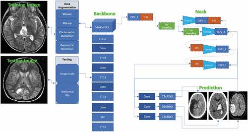
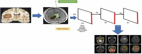
Figure 1 shows the i-YOLOV5 architectural model (Bernal et al. 2019). Three parts together make up the architecture: (i) Backbone, (ii) Neck, and (iii) Prediction.

1. Backbone: VGG, ResNet, DenseNet, MobileNet, EfficientNet, CSPDarknet53, Swin Transformer, and other backbones are frequently utilized instead of our networks. Since these networks have demonstrated that they can extract useful features for classification and other tasks, researchers will fine-tune the Backbone to better suit various jobs.

2. Neck: The neck is intended to increase the benefits of the Backbone’s qualities. It reprocesses and utilizes the feature maps extracted by Backbone at various stages intelligently. A neck is typically processed by many top-down and bottom-up approaches. The target detection architecture relies heavily on the neck. The usage of an up-and-down sampling block is the first neck. The advantage of this strategy is that no feature layer aggregation process, such as SSD, follows the multi-level feature map straight after the head. FPN, PANet, NAS-FPN, BiFPN, ASFF, and SFAM are the most used path-aggregation blocks in the neck. The employment of diverse up-and-down sampling, splicing, dot sum, and the dot product to construct aggregation algorithms is similar to these methods. SPP, ASPP, RFB, and CBAM are some other blocks utilized in the neck.

3. Prediction: Because the backbone cannot fulfil the positioning task as a classification network, the head is designed to detect the object’s location and category using feature maps acquired from the backbone. There are two object detector heads: one-stage and two-stage object detectors. The RCNN series is representative of two-stage detectors, which have long been the dominating method in object detection. The one-stage detector, as compared to the two-stage detector, forecasts the BB and object class at the same time. The one-stage detector has a clear speed advantage, but its accuracy is reduced. The most prominent models for one-stage detectors are the YOLO series, SSD, and RetinaNet. i-YOLOV5 is also significantly faster than prior YOLO versions. Furthermore, when compared to YOLO4, i-YOLO-5 is roughly lesser than 90.24%. This makes it much easier to deploy i-YOLOV5 to embedded devices.

Figure 1. A Proposed i-YOLOV5 Model for BT Detection to Feature Extraction.

Mosaic Data Enhancement

The same Mosaic Data Enhancement approach is used at the input end of i-YOLOV5 (Figure 2).

Figure 2. Enhancement approach of Mosaic Image Processing.

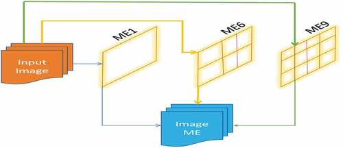
Arithmetic progression with tiny targets is part of the formal project training. Goals are often smaller than medium-to-big goals (Fu et al. 2020). The data collected by us has a wide range of small objectives. However, the allocation of small targets is uneven, which is more problematic. Numerous features such as random distribution for splicing, random scaling, random utilization images, and rich data sets considerably enhance the data set in performing detection. In particular, random scaling is used to turn the network into a highly durable one. This adds a few small targets. There is a possibility that a few people argue that random scaling or simple data enhancements could be performed while lowering GPU. However, because many individuals may own a GPU, the data associated with four photographs could be quickly computed using Mosaic enhancement training by reducing the Mini-batch size to a manageable level. As a result, a GPU can produce better outcomes.

Adaptive Anchor Frame Calculation

The YOLO consists of an Anchor frame with a starting length and width in the YOLO method for different data sets. During the network training stage, the primary anchor frame prediction frame is nothing but the network outputs. Then, the Ground Truth (GT) comparison is determined (Jocher 2020) performance improvements. Later, the modification of iterative network parameters is carried out in reverse. While training various data sets in YOLO3 and YOLO4, calculating the initial anchor box value is performed using a different application. In i-YOLOV5, however, this method is built into the code. As a result, during each step in training, the best anchor box value is calculated and changed adaptively.

Adaptive Image Scaling

The size and shape of a target object can be proven in varying methods, but the most common technique is to scale the actual images to regular size before feeding them to the detection network (Kaur, Saini, and Gupta 2019). After zooming and filling, many defective images may significantly impact the effectiveness and black image boundaries. Information redundancy will occur if more fills are required, slowing down reasoning speed. As a result, in the i-YOLOV5 code, the letterbox function in the YOLOV5 code is adaptively adapted to the input images, and the most miniature black border differs from our prior research work. The black edges at both ends of the image height have been lowered, resulting in fewer calculations during inference and faster target detection. The inference speed was already enhanced by 40% due to this simple change, which is quite successful.

The Detection Approach

Using CV to detect minor flaws in noisy images of BT is quite challenging. In a noisy image’s feature space, the presence of high gradient magnitude and short duration are the main traits of BT. The following qualities might be considered to improve and get noise-free images for identifying brain tumors.

Anisotropic Diffusion Filter

In enhancing image applications, an anisotropic diffusion filter is commonly utilized. Once again, the edges from the brain image are eliminated, and a mask is built using the filtration method to detect the precise tissue location (Van Leemput et al. 2001). It uses spatial information to filter, lowering the noise level. Equation (1)(1) ${\mathrm{S}}_{\mathrm{P}\mathrm{x}\mathrm{l}}^{\mathrm{i}+1}{=1}_{\mathrm{P}\mathrm{x}\mathrm{l}}^{\mathrm{i}}+\frac{\alpha }{⌈{\alpha }_{\mathrm{P}\mathrm{x}\mathrm{l}}⌉}\sum _{{\mathrm{k}}^{\mathrm{o}}{\alpha }_{\mathrm{P}\mathrm{x}\mathrm{l}}}\mathrm{f}\mathrm{u}\mathrm{n}(\left|{\mathrm{\Delta }\mathrm{S}}_{\mathrm{P}\mathrm{x}\mathrm{l},\mathrm{k}}^{\mathrm{i}}\right|,\lambda ){\mathrm{\Delta }\mathrm{S}}_{\mathrm{P}\mathrm{x}\mathrm{l},\mathrm{k}}^{\mathrm{i}}$(1) gives the discrete function of an anisotropic filter where “S” denotes the pixel “Pxl” test case “i” based strength level.

(1) ${\mathrm{S}}_{\mathrm{P}\mathrm{x}\mathrm{l}}^{\mathrm{i}+1}{=1}_{\mathrm{P}\mathrm{x}\mathrm{l}}^{\mathrm{i}}+\frac{\alpha }{⌈{\alpha }_{\mathrm{P}\mathrm{x}\mathrm{l}}⌉}\sum _{{\mathrm{k}}^{\mathrm{o}}{\alpha }_{\mathrm{P}\mathrm{x}\mathrm{l}}}\mathrm{f}\mathrm{u}\mathrm{n}(\left|{\mathrm{\Delta }\mathrm{S}}_{\mathrm{P}\mathrm{x}\mathrm{l},\mathrm{k}}^{\mathrm{i}}\right|,\lambda ){\mathrm{\Delta }\mathrm{S}}_{\mathrm{P}\mathrm{x}\mathrm{l},\mathrm{k}}^{\mathrm{i}}$(1)

In this case, $fun(\left|\mathrm{\Delta }{S}_{Pxl,k}^i\right|,\lambda )$it is the scalar diffusion function. ’Pxl ‘is $\mathrm{\Delta }{S}_{Pxl,k}^i$ the smoothing level of various pixels. The forward and backward differences are performed to estimate the value using the diffusion coefficient. Equation (2)(2) ${\mathrm{D}\mathrm{C}(\mathrm{S}}_{\mathrm{x},\mathrm{k}}^{\mathrm{i}}{-\mathrm{S}}_{\mathrm{y},\mathrm{l}}^{\mathrm{i}})=\frac{(\mathrm{I}\mathrm{m}{\mathrm{g}}_{\mathrm{b}}\mathrm{x},\mathrm{k}+\mathrm{I}\mathrm{m}{\mathrm{g}}_{\mathrm{b}}\mathrm{y},\mathrm{l})}{2}$(2) is provided by,

(2) ${\mathrm{D}\mathrm{C}(\mathrm{S}}_{\mathrm{x},\mathrm{k}}^{\mathrm{i}}{-\mathrm{S}}_{\mathrm{y},\mathrm{l}}^{\mathrm{i}})=\frac{(\mathrm{I}\mathrm{m}{\mathrm{g}}_{\mathrm{b}}\mathrm{x},\mathrm{k}+\mathrm{I}\mathrm{m}{\mathrm{g}}_{\mathrm{b}}\mathrm{y},\mathrm{l})}{2}$(2)

The variables represent the noisy brain image that consists of four different neighborhood pixels x, y, k, and l. The weak pixels are used to accomplish the diffusion action. The diffusion coefficient has been applied to the marked segmented region. The diffused image is transformed into a binary image, and the brain region is separated. Before accepting the threshold value that maps out where the tissue is, the enhanced filtering method reduces the number of pixels that come after it. Equation (3) and Equation (4) are the eigenvalues of “De” and their corresponding eigenvectors.

$(\mathrm{c}\mathrm{o}\mathrm{s}\psi ,\mathrm{s}\mathrm{i}\mathrm{n}\psi )\mathrm{a}\mathrm{n}\mathrm{d}(\mathrm{c}\mathrm{o}{\mathrm{s}}^{-1}\psi ,\mathrm{s}\mathrm{i}{\mathrm{n}}^{-1}\psi )$, where $y[-\frac{\mathrm{p}/2}{\mathrm{p}/2}]$ (3)

(4) $Div({\mathrm{D}}_e,{ }^{\prime \prime }{ }_u)={\mathrm{a}}_{\mathrm{b}}({\mathrm{a}}_0{\mathrm{d}}_{\mathrm{b}}\mathrm{u})$(4)

Here the partition $-\frac{\pi /2}{\pi /2}$ will be followed as Equation (5)(5) $\left[-\frac{\pi }{2},\frac{\pi }{2}\right]=(-\frac{\pi }{2},0)\text{amp}(\frac{\pi }{2},0)$(5) and Equation (6)(6) $\left[-\frac{\pi }{2},\frac{\pi }{2}\right]=-S\text{amp}S$(6)

(5) $\left[-\frac{\pi }{2},\frac{\pi }{2}\right]=(-\frac{\pi }{2},0)\text{amp}(\frac{\pi }{2},0)$(5)

(6) $\left[-\frac{\pi }{2},\frac{\pi }{2}\right]=-S\text{amp}S$(6)

The weight function of the tumor region is mapped using the grid angle of a probability distribution function. Equation (7)(7) $P(\mathrm{x},\mathrm{y}){\mathrm{a}}_{\mathrm{x}}\mathrm{u}+2\mathrm{Q}(\mathrm{x},\mathrm{y}){\mathrm{a}}_{\mathrm{y}}\mathrm{u}+\mathrm{R}(\mathrm{x},\mathrm{y}){\mathrm{a}}_{\mathrm{z}}\mathrm{u}$(7) is a nonnegative approximation value.

(7) $P(\mathrm{x},\mathrm{y}){\mathrm{a}}_{\mathrm{x}}\mathrm{u}+2\mathrm{Q}(\mathrm{x},\mathrm{y}){\mathrm{a}}_{\mathrm{y}}\mathrm{u}+\mathrm{R}(\mathrm{x},\mathrm{y}){\mathrm{a}}_{\mathrm{z}}\mathrm{u}$(7)

In the filtering procedure, the discrete diffusion function is used. The symmetrical property is added to the discrete image after grayscale scaling. To smooth the image, the average gray value, which is given by Equation (8)(8) $GrayValu{e}_{avg}=\frac{1}{T}\sum { }_{i=j}f(i)$(8) , is chosen.

(8) $GrayValu{e}_{avg}=\frac{1}{T}\sum { }_{i=j}f(i)$(8)

The mathematical model is represented as Equation (9)(9) $\frac{1}{T}\sum { }_{i=j}{u}^j(i)=\mathrm{G}\mathrm{r}\mathrm{a}\mathrm{y}\mathrm{V}\mathrm{a}\mathrm{l}\mathrm{u}{\mathrm{e}}_{\mathrm{a}\mathrm{v}\mathrm{g}}$(9) after the anisotropic filter is filtered by diffusion,

(9) $\frac{1}{T}\sum { }_{i=j}{u}^j(i)=\mathrm{G}\mathrm{r}\mathrm{a}\mathrm{y}\mathrm{V}\mathrm{a}\mathrm{l}\mathrm{u}{\mathrm{e}}_{\mathrm{a}\mathrm{v}\mathrm{g}}$(9)

The tumor size is tiny here on the MRI brain image; the specific tumor location is determined based on firmness and area. The area of the tumor can be found by comparing the image with the black-and-white image.

The detection method of the i-YOLOV5-based model is briefly described in this section. The model begins by analyzing an image and calculating a probability on a cell area using logical SxS grids and weighted feature sets. If the center of a possible item falls into one of the cells, a preliminary BB is generated using the prediction probability provided by the trained model in Equation (10)(12) ${\mathrm{I}\mathrm{n}\mathrm{t}\mathrm{e}\mathrm{r}\mathrm{s}\mathrm{e}\mathrm{c}\mathrm{t}\mathrm{i}\mathrm{o}\mathrm{n}\mathrm{O}\mathrm{v}\mathrm{e}\mathrm{r}\mathrm{U}\mathrm{n}\mathrm{i}\mathrm{o}\mathrm{n}}_{\mathrm{P}\mathrm{r}\mathrm{e}\mathrm{d}\mathrm{i}\mathrm{c}\mathrm{t}\mathrm{e}\mathrm{d}}^{\mathrm{T}\mathrm{r}\mathrm{u}\mathrm{e}}=\frac{\mathrm{A}\mathrm{r}\mathrm{e}\mathrm{a}\mathrm{o}\mathrm{f}\mathrm{I}\mathrm{m}\mathrm{a}\mathrm{g}\mathrm{e}(B^{\mathrm{T}\mathrm{r}\mathrm{u}\mathrm{e}}\cap B^{\mathrm{P}\mathrm{r}\mathrm{e}\mathrm{d}\mathrm{i}\mathrm{c}\mathrm{t}\mathrm{e}\mathrm{d}})}{\mathrm{A}\mathrm{r}\mathrm{e}\mathrm{a}\mathrm{o}\mathrm{f}\mathrm{I}\mathrm{m}\mathrm{a}\mathrm{g}\mathrm{e}(B^{\mathrm{T}\mathrm{r}\mathrm{u}\mathrm{e}}\cap B^{\mathrm{P}\mathrm{r}\mathrm{e}\mathrm{d}\mathrm{i}\mathrm{c}\mathrm{t}\mathrm{e}\mathrm{d}})}$(12) .$\mathrm{P}\mathrm{r}\mathrm{o}\mathrm{b}(\mathrm{O}\mathrm{b}\mathrm{j})=\left\{\begin{array}{c}{0}_{\mathrm{W}\mathrm{i}\mathrm{t}\mathrm{h}\mathrm{P}\mathrm{o}\mathrm{t}\mathrm{e}\mathrm{n}\mathrm{t}\mathrm{i}\mathrm{a}\mathrm{l}}\\ 1_{\mathrm{W}\mathrm{i}\mathrm{t}\mathrm{h}\mathrm{o}\mathrm{u}\mathrm{t}\mathrm{P}\mathrm{o}\mathrm{t}\mathrm{e}\mathrm{n}\mathrm{t}\mathrm{i}\mathrm{a}\mathrm{l}}\end{array}\right\}$ (10)

The model following forecasts multiple scaled boxes using “K” and extracts a 3D tensor using Equation (11)(11) $S\times S\times (k\times (2+1+c)$(11) , where C is the defined number of classes, four denotes the T_x,T_y,T_w,T_ℎ BB prediction coordinates, and one denotes the confidence of prediction for each BB.

(11) $S\times S\times (k\times (2+1+c)$(11)

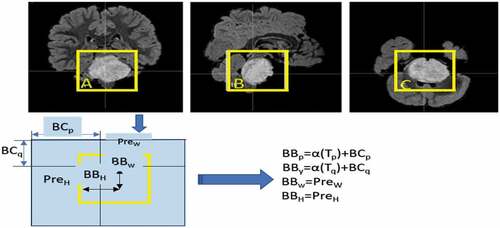
The BB prediction is based on the width Pxl_w and height Pxl_ℎ in Figure 3 with C_x and C_y offsets from the cluster centroid. The prediction corresponds to the BB model when the cell is offset from the upper left by (c_x, c_y) and the BB has values of Pxl_w and Pxl_h.

Figure 3. Bounding Box Prediction with tumor specifications.

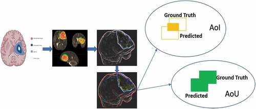
During the generation of BB, the Intersection Over Union (IoU) in Equation (12)(12) ${\mathrm{I}\mathrm{n}\mathrm{t}\mathrm{e}\mathrm{r}\mathrm{s}\mathrm{e}\mathrm{c}\mathrm{t}\mathrm{i}\mathrm{o}\mathrm{n}\mathrm{O}\mathrm{v}\mathrm{e}\mathrm{r}\mathrm{U}\mathrm{n}\mathrm{i}\mathrm{o}\mathrm{n}}_{\mathrm{P}\mathrm{r}\mathrm{e}\mathrm{d}\mathrm{i}\mathrm{c}\mathrm{t}\mathrm{e}\mathrm{d}}^{\mathrm{T}\mathrm{r}\mathrm{u}\mathrm{e}}=\frac{\mathrm{A}\mathrm{r}\mathrm{e}\mathrm{a}\mathrm{o}\mathrm{f}\mathrm{I}\mathrm{m}\mathrm{a}\mathrm{g}\mathrm{e}(B^{\mathrm{T}\mathrm{r}\mathrm{u}\mathrm{e}}\cap B^{\mathrm{P}\mathrm{r}\mathrm{e}\mathrm{d}\mathrm{i}\mathrm{c}\mathrm{t}\mathrm{e}\mathrm{d}})}{\mathrm{A}\mathrm{r}\mathrm{e}\mathrm{a}\mathrm{o}\mathrm{f}\mathrm{I}\mathrm{m}\mathrm{a}\mathrm{g}\mathrm{e}(B^{\mathrm{T}\mathrm{r}\mathrm{u}\mathrm{e}}\cap B^{\mathrm{P}\mathrm{r}\mathrm{e}\mathrm{d}\mathrm{i}\mathrm{c}\mathrm{t}\mathrm{e}\mathrm{d}})}$(12) represents whether the prediction nearly maps a GT image from a dataset. When the first predicted object doesn’t closely match the GT, the confidence score drops, resulting in a dissatisfied prediction. According to Equation (13)(13) $\mathrm{C}\mathrm{o}\mathrm{n}\mathrm{f}\mathrm{i}\mathrm{d}\mathrm{e}\mathrm{n}\mathrm{c}\mathrm{e}(Obj)=\mathrm{P}\mathrm{r}\mathrm{e}\mathrm{d}\mathrm{i}\mathrm{c}\mathrm{a}\mathrm{t}\mathrm{e}\mathrm{V}\mathrm{a}\mathrm{l}\mathrm{u}\mathrm{e}(Obj)\times {\mathrm{I}\mathrm{n}\mathrm{t}\mathrm{e}\mathrm{r}\mathrm{s}\mathrm{e}\mathrm{c}\mathrm{t}\mathrm{i}\mathrm{o}\mathrm{n}\mathrm{O}\mathrm{v}\mathrm{e}\mathrm{r}\mathrm{U}\mathrm{n}\mathrm{i}\mathrm{o}\mathrm{n}}_{\mathrm{P}\mathrm{r}\mathrm{e}\mathrm{d}\mathrm{i}\mathrm{c}\mathrm{t}\mathrm{e}\mathrm{d}}^{\mathrm{T}\mathrm{r}\mathrm{u}\mathrm{e}}$(13) , Figure 4 gives a graphic example of how the IoU evaluates an object, with the Ground Truth (GT) and a probable detection outcome from the algorithm surrounded by a BB.

Figure 4. Ground Truth Test for Brain Tumor Detection.

(12) ${\mathrm{I}\mathrm{n}\mathrm{t}\mathrm{e}\mathrm{r}\mathrm{s}\mathrm{e}\mathrm{c}\mathrm{t}\mathrm{i}\mathrm{o}\mathrm{n}\mathrm{O}\mathrm{v}\mathrm{e}\mathrm{r}\mathrm{U}\mathrm{n}\mathrm{i}\mathrm{o}\mathrm{n}}_{\mathrm{P}\mathrm{r}\mathrm{e}\mathrm{d}\mathrm{i}\mathrm{c}\mathrm{t}\mathrm{e}\mathrm{d}}^{\mathrm{T}\mathrm{r}\mathrm{u}\mathrm{e}}=\frac{\mathrm{A}\mathrm{r}\mathrm{e}\mathrm{a}\mathrm{o}\mathrm{f}\mathrm{I}\mathrm{m}\mathrm{a}\mathrm{g}\mathrm{e}(B^{\mathrm{T}\mathrm{r}\mathrm{u}\mathrm{e}}\cap B^{\mathrm{P}\mathrm{r}\mathrm{e}\mathrm{d}\mathrm{i}\mathrm{c}\mathrm{t}\mathrm{e}\mathrm{d}})}{\mathrm{A}\mathrm{r}\mathrm{e}\mathrm{a}\mathrm{o}\mathrm{f}\mathrm{I}\mathrm{m}\mathrm{a}\mathrm{g}\mathrm{e}(B^{\mathrm{T}\mathrm{r}\mathrm{u}\mathrm{e}}\cap B^{\mathrm{P}\mathrm{r}\mathrm{e}\mathrm{d}\mathrm{i}\mathrm{c}\mathrm{t}\mathrm{e}\mathrm{d}})}$(12)

(13) $\mathrm{C}\mathrm{o}\mathrm{n}\mathrm{f}\mathrm{i}\mathrm{d}\mathrm{e}\mathrm{n}\mathrm{c}\mathrm{e}(Obj)=\mathrm{P}\mathrm{r}\mathrm{e}\mathrm{d}\mathrm{i}\mathrm{c}\mathrm{a}\mathrm{t}\mathrm{e}\mathrm{V}\mathrm{a}\mathrm{l}\mathrm{u}\mathrm{e}(Obj)\times {\mathrm{I}\mathrm{n}\mathrm{t}\mathrm{e}\mathrm{r}\mathrm{s}\mathrm{e}\mathrm{c}\mathrm{t}\mathrm{i}\mathrm{o}\mathrm{n}\mathrm{O}\mathrm{v}\mathrm{e}\mathrm{r}\mathrm{U}\mathrm{n}\mathrm{i}\mathrm{o}\mathrm{n}}_{\mathrm{P}\mathrm{r}\mathrm{e}\mathrm{d}\mathrm{i}\mathrm{c}\mathrm{t}\mathrm{e}\mathrm{d}}^{\mathrm{T}\mathrm{r}\mathrm{u}\mathrm{e}}$(13)

Predicted_Value (Class_i |Obj) is used to determine “C” for each grid cell. Only objects that fulfil the provided threshold will receive an initial BB, even if several predictions are made for the same object. The following is presented precisely by Equation (14)(14) $\begin{array}{rl}& \mathrm{P}\mathrm{r}\mathrm{e}\mathrm{d}\mathrm{i}\mathrm{c}\mathrm{a}\mathrm{t}\mathrm{e}\mathrm{V}\mathrm{a}\mathrm{l}\mathrm{u}\mathrm{e}(Clas{s}_i|Obj)\times {\mathrm{I}\mathrm{n}\mathrm{t}\mathrm{e}\mathrm{r}\mathrm{s}\mathrm{e}\mathrm{c}\mathrm{t}\mathrm{i}\mathrm{o}\mathrm{n}\mathrm{O}\mathrm{v}\mathrm{e}\mathrm{r}\mathrm{U}\mathrm{n}\mathrm{i}\mathrm{o}\mathrm{n}}_{\mathrm{P}\mathrm{r}\mathrm{e}\mathrm{d}\mathrm{i}\mathrm{c}\mathrm{t}\mathrm{e}\mathrm{d}}^{\mathrm{T}\mathrm{r}\mathrm{u}\mathrm{e}}\\ & =\mathrm{P}\mathrm{r}\mathrm{e}\mathrm{d}\mathrm{i}\mathrm{c}\mathrm{a}\mathrm{t}\mathrm{e}\mathrm{V}\mathrm{a}\mathrm{l}\mathrm{u}\mathrm{e}(Clas{s}_i)\times {\mathrm{I}\mathrm{n}\mathrm{t}\mathrm{e}\mathrm{r}\mathrm{s}\mathrm{e}\mathrm{c}\mathrm{t}\mathrm{i}\mathrm{o}\mathrm{n}\mathrm{O}\mathrm{v}\mathrm{e}\mathrm{r}\mathrm{U}\mathrm{n}\mathrm{i}\mathrm{o}\mathrm{n}}_{\mathrm{P}\mathrm{r}\mathrm{e}\mathrm{d}\mathrm{i}\mathrm{c}\mathrm{t}\mathrm{e}\mathrm{d}}^{\mathrm{T}\mathrm{r}\mathrm{u}\mathrm{e}}\end{array}$(14) .

(14) $\begin{array}{rl}& \mathrm{P}\mathrm{r}\mathrm{e}\mathrm{d}\mathrm{i}\mathrm{c}\mathrm{a}\mathrm{t}\mathrm{e}\mathrm{V}\mathrm{a}\mathrm{l}\mathrm{u}\mathrm{e}(Clas{s}_i|Obj)\times {\mathrm{I}\mathrm{n}\mathrm{t}\mathrm{e}\mathrm{r}\mathrm{s}\mathrm{e}\mathrm{c}\mathrm{t}\mathrm{i}\mathrm{o}\mathrm{n}\mathrm{O}\mathrm{v}\mathrm{e}\mathrm{r}\mathrm{U}\mathrm{n}\mathrm{i}\mathrm{o}\mathrm{n}}_{\mathrm{P}\mathrm{r}\mathrm{e}\mathrm{d}\mathrm{i}\mathrm{c}\mathrm{t}\mathrm{e}\mathrm{d}}^{\mathrm{T}\mathrm{r}\mathrm{u}\mathrm{e}}\\ & =\mathrm{P}\mathrm{r}\mathrm{e}\mathrm{d}\mathrm{i}\mathrm{c}\mathrm{a}\mathrm{t}\mathrm{e}\mathrm{V}\mathrm{a}\mathrm{l}\mathrm{u}\mathrm{e}(Clas{s}_i)\times {\mathrm{I}\mathrm{n}\mathrm{t}\mathrm{e}\mathrm{r}\mathrm{s}\mathrm{e}\mathrm{c}\mathrm{t}\mathrm{i}\mathrm{o}\mathrm{n}\mathrm{O}\mathrm{v}\mathrm{e}\mathrm{r}\mathrm{U}\mathrm{n}\mathrm{i}\mathrm{o}\mathrm{n}}_{\mathrm{P}\mathrm{r}\mathrm{e}\mathrm{d}\mathrm{i}\mathrm{c}\mathrm{t}\mathrm{e}\mathrm{d}}^{\mathrm{T}\mathrm{r}\mathrm{u}\mathrm{e}}\end{array}$(14)

Numerous possible object predictions can arise in most circumstances during the initial detection. Using the Non-Maximum Suppression technique, the detection model could keep just the prediction with the most significant confidence score and efficiently eliminate any redundant boxes. The proposed YOLOV5-based model’s detection method is depicted in Figure 5.

Figure 5. The proposed i-YOLOV5 model for Brain Tumor Detection.

Localization

The i- YOLOV5 model with 174 layers have 1 input, 50 conv, 50 bn, 50 linear activations ReLU, 7 mixed (depth concatenation), 4 max-pooling, 6 average pooling, and 10 layers of the i-YOLOV5 model are proposed to localize tumor region. Table 2 shows the optimal hyper-parameters.

Table 2. Optimal Hyper Parameters of proposed YOLOV5.

Parameter	Threshold
Epochs	30
Batch-size	15
Rate of Learning	0.0013
Momentum	0.981
Optimizer	SGD

The tumor location is localized by the proposed model in a more precise manner, as seen in Figure 4, with the help of the i-YOLOV5 model, optimizing the MSE loss between due bounds and GT boxes.

Localization, confidence, and classification are the three main kinds of losses utilized for training. The prediction of box size, error utilizing location, and GT between the anticipated and GT boxes are computed using localization loss. Moreover, the confidence loss is used to compute the objectiveness error for detected objects in the j^th BB of grid “i” cell. The classification loss is employed to determine chance over every class of grid cell “i.” Equation (15)(15) $\begin{array}{rl}& Weigh{t_1}_{i=0}^{g{c}^2}\sum _{i,j}^{Box}{1}_{i,j}^{Obj}[x_i+\overline{x_i}{]}^2-[y_i+\overline{y_i}{]}^2+\\ & Weigh{t}_1\sum _{i=0}^{g{c}^2}\sum _{i,j}^{Box}{1}_{i,j}^{Obj}[W_i-\overline{W_j}{]}^2+[H_i-\overline{H_j}{]}^2+\\ & Weigh{t}_3\sum _{i=0}^{g{c}^2}\sum _{i,j}^{Box}{1}_{i,j}^{Obj}[C{S}_i-\overline{C{S}_j}{]}^2+\\ & Weigh{t}_4\sum _{i=0}^{g{c}^2}\sum _{i,j}^{Box}{1}_{i,j}^{Obj}[\mathrm{P}\mathrm{r}\mathrm{o}\mathrm{b}(C{)}_i-\overline{Prob{(C)}_j}{]}^2+\end{array}$(15) expresses the mathematical equation of these parameters:

(15) $\begin{array}{rl}& Weigh{t_1}_{i=0}^{g{c}^2}\sum _{i,j}^{Box}{1}_{i,j}^{Obj}[x_i+\overline{x_i}{]}^2-[y_i+\overline{y_i}{]}^2+\\ & Weigh{t}_1\sum _{i=0}^{g{c}^2}\sum _{i,j}^{Box}{1}_{i,j}^{Obj}[W_i-\overline{W_j}{]}^2+[H_i-\overline{H_j}{]}^2+\\ & Weigh{t}_3\sum _{i=0}^{g{c}^2}\sum _{i,j}^{Box}{1}_{i,j}^{Obj}[C{S}_i-\overline{C{S}_j}{]}^2+\\ & Weigh{t}_4\sum _{i=0}^{g{c}^2}\sum _{i,j}^{Box}{1}_{i,j}^{Obj}[\mathrm{P}\mathrm{r}\mathrm{o}\mathrm{b}(C{)}_i-\overline{Prob{(C)}_j}{]}^2+\end{array}$(15)

The letters for the grid cell are s, the probability is p, weights are represented by W1, W2, W3, and W4 and the grid cell is presented by GC. ($\hat{x}$_i , Ŷ is the center of the BB, and (xi, yi) is the center of the GT. (W_i, H_i) signifies the width and height of the BB, while (W_i, H_i) denotes the width and height of the GT. The eroded image turns each neighborhood area into a black-point zone. The detected image edges are demonstrated when an eroded image is derived from the actual image source. The diffusion rate is managed here using the BB process to preserve the edge rate. Equation (16)(16) $CD(\left|\mathrm{\Delta }\right|)=Exp(-\frac{(\left|\mathrm{\Delta }\right|)}{k}{)}^2$(16) is used to calculate the diffusion coefficient.

(16) $CD(\left|\mathrm{\Delta }\right|)=Exp(-\frac{(\left|\mathrm{\Delta }\right|)}{k}{)}^2$(16)

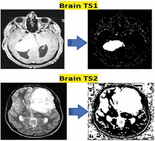
Lesion Segmentation

In medical imaging, the most challenging aspect is the variation in medical data. Human anatomy witnesses the variances shown by distinct modalities like PET, MRI, CT, and X-Ray. The segmentation area is the primary source for analyzing the levels of seriousness of the disease. The proposed method segments the tumors using McCulloch’s Kapur Entropy Method (MKEM) (Li et al. 2021; Liang, Liang et al. 2017; Louis, David N Louis et al. 2016; Narmatha et al. 2020; Pan et al. 2015). The chance of intensity value distributions of the foreground and background regions is calculated in this method, and the value of entropy is independent for both, as shown in Figure 6. The use of an optimum threshold value enhances total entropy. Equation (17)(17) $\begin{array}{rl}& Randomnes{s}_0=-\sum _{i=0}^{T_1-1}(\frac{\mathrm{P}\mathrm{r}\mathrm{o}{\mathrm{b}}_i}{{\omega }_o})+Lo{g}_2(\frac{\mathrm{P}\mathrm{r}\mathrm{o}{\mathrm{b}}_i}{{\omega }_o})+\\ & Randomnes{s}_1-\sum _{i=0}^{T_2-1}(\frac{\mathrm{P}\mathrm{r}\mathrm{o}{\mathrm{b}}_i}{{\omega }_o})+Lo{g}_2(\frac{\mathrm{P}\mathrm{r}\mathrm{o}{\mathrm{b}}_i}{{\omega }_o})+\\ & Randomnes{s}_i-\sum _{i=T_i}^{Ti+1^{-1}}(\frac{\mathrm{P}\mathrm{r}\mathrm{o}{\mathrm{b}}_i}{{\omega }_o})+Lo{g}_2(\frac{\mathrm{P}\mathrm{r}\mathrm{o}{\mathrm{b}}_i}{{\omega }_o})+\\ & Randomnes{s}_j-\sum _{i=T_j}^{N-1}(\frac{\mathrm{P}\mathrm{r}\mathrm{o}{\mathrm{b}}_i}{{\omega }_o})+Lo{g}_2(\frac{\mathrm{P}\mathrm{r}\mathrm{o}{\mathrm{b}}_i}{{\omega }_o})\end{array}$(17) is the mathematical expression of the MKEM:

(17) $\begin{array}{rl}& Randomnes{s}_0=-\sum _{i=0}^{T_1-1}(\frac{\mathrm{P}\mathrm{r}\mathrm{o}{\mathrm{b}}_i}{{\omega }_o})+Lo{g}_2(\frac{\mathrm{P}\mathrm{r}\mathrm{o}{\mathrm{b}}_i}{{\omega }_o})+\\ & Randomnes{s}_1-\sum _{i=0}^{T_2-1}(\frac{\mathrm{P}\mathrm{r}\mathrm{o}{\mathrm{b}}_i}{{\omega }_o})+Lo{g}_2(\frac{\mathrm{P}\mathrm{r}\mathrm{o}{\mathrm{b}}_i}{{\omega }_o})+\\ & Randomnes{s}_i-\sum _{i=T_i}^{Ti+1^{-1}}(\frac{\mathrm{P}\mathrm{r}\mathrm{o}{\mathrm{b}}_i}{{\omega }_o})+Lo{g}_2(\frac{\mathrm{P}\mathrm{r}\mathrm{o}{\mathrm{b}}_i}{{\omega }_o})+\\ & Randomnes{s}_j-\sum _{i=T_j}^{N-1}(\frac{\mathrm{P}\mathrm{r}\mathrm{o}{\mathrm{b}}_i}{{\omega }_o})+Lo{g}_2(\frac{\mathrm{P}\mathrm{r}\mathrm{o}{\mathrm{b}}_i}{{\omega }_o})\end{array}$(17)

Figure 6. Segmented Lesion Zone of Input Image.

Hyper-Parameter Optimization (HPO)

The growing demand for medical image processing using CNNs has stimulated various challenges in applying CNNs. Since achieving more significant results using specially designed architectures is so profound, the cost of computing becomes high, and the quality of input images becomes higher. The advanced hardware and HPO of the extensive network are critical for reducing these computation expenses and achieving more successful results. Consequently, all the complicated HP of the proposed CNN models are tuned automatically using the HGSOA. When the value range is modest, the HGSOA is an excellent alternative to CNN’s HPO. The HPO algorithm seeks to find the range of combinations that is the best combination in which training can be provided to the Yolo v5 network (Begum and Lakshmi 2020; Pei et al. 2020, 2020; Philip Bachman and Buchwalter 2019).

CNN models are complex architectures with hyper-parameters in large numbers. Mostly, architectural and fine adjustment are the two often classified as HPO. Activation function, convolutional pooling layers, ultimately linked layers, filters, and sizes comprise architectural HPO. On the other hand, momentum, learning rate, and 12 regularizations are included in the Fine adjustment HPO. This work uses HGSOA to tune fine adjustment HPO once the architectural HPO is tuned.

Algorithm for HGSOA to Optimize Tuned and Fine Adjustment of HPO

Step 1. Set 3D grid for HPO to be optimized

• (a) No. of Conv and Max Pooling Layers for Regulation

• (b) No. of FC Layers

• (c) No. of Filters

• (d) Filter Sizes

• (e) Momentum, Batch Size and Learning Rate

Step 2. Set potential value intervals corresponding to each dimension

• (a) No. of Conv and Max Pooling Layers [1 to 4]

• (b) No. of FC Layers [1 to 4]

• (c) No. of Filters [8, 16, 24, 32, 40, 48, 56, 64, 72, 80, 88, 96]

• (d) Filter Size [2, 4, 6, 8, 10]

• (e) Ensure Activation Function

• (f) Regulation and Learning Rate {0.0001, 0.0006, 0.0002, 0.0008}

Step 3. Search for all the candidate combinations

• (a) Choose to optimize accuracy

• (b) I1, I2, I3 → Accuracy (97, 98, 99,)

McCulloch’s Algorithm for Segmentation

Regarding random walk-in McCulloch’s cuckoo searches, levy flight has devised a new strategy. A much more efficient and cheaper method for obtaining stable random variables that can use the model levy flight is proposed in the proposed method. This method improves the cuckoo search method’s convergence rate and efficiency in time-constrained situations. Many effective random number generation methods have been proposed, with most relying on the inverse distribution of a collection of uniformly distributed (in the range of 0–1) pseudo-random numbers. In the levy flight approach deployed in this proposed work, there is a function of an exponential value with a “c” scaling parameter, “β” skewness measurement, and “δ” position specification parameter. A matrix PxQ of random value is denoted by an exponential value (Azizi et al. 2021; Liu et al. 2018; Shukla et al. 2017; Solawetz 2020). The proposed approach’s cost of generating a constant random number is lower. A PxQ matrix of random numbers that are distinguished using “α” exponential values, “c” scaling parameter, and skewness measurement are applied by our proposed method. “β” and “a” location parameter “δ.” Various degrees of the algorithm have been explained using the parameter “α” where “S” stands for the step size Equation (18)(18) $Siz{e}_x=Compute[\frac{sin(\alpha \varphi +{tan}^{-1}(\beta tan(\frac{\alpha \pi }{2})+cos(1-\alpha )\varphi +{tan}^{-1}(\beta tan(\frac{\alpha \pi }{2})}{cos({tan}^{-1}(\beta tan(\frac{\alpha \pi }{2})+cos{(\varphi )}^{\frac{1}{\alpha }\omega -1}+\delta \sim S_{\alpha }(c,\beta ,\lambda )}]$(18) .

(18) $Siz{e}_x=Compute[\frac{sin(\alpha \varphi +{tan}^{-1}(\beta tan(\frac{\alpha \pi }{2})+cos(1-\alpha )\varphi +{tan}^{-1}(\beta tan(\frac{\alpha \pi }{2})}{cos({tan}^{-1}(\beta tan(\frac{\alpha \pi }{2})+cos{(\varphi )}^{\frac{1}{\alpha }\omega -1}+\delta \sim S_{\alpha }(c,\beta ,\lambda )}]$(18)

Step 1. α = 1 of “δ”

Step 2. s = c * Tan(φ) + δ

Step 3. α = 2 matches the Gaussian with mean as “δ” and variance are given by 2*c2

Step 4. s = 2 * c√ѡ * Sin (φ) + δ

Step 5. α > 1 produces the mean of the distribution to be “δ” for all values of “β”, where

Step 6. ѡ = −Log₁₀ * (Random (P, Q)) and φ = Random (P, Q) – (1, 2) * π

The algorithm computes step sizes using the above formula for β = 0 and α = 1.

α = 0.5 and β = 0 were chosen for our investigation. To avoid overflow should be kept between 0 and 2.

Equation (19)(23) $\mathrm{M}\mathrm{e}\mathrm{a}\mathrm{n}\mathrm{S}\mathrm{q}\mathrm{u}\mathrm{a}\mathrm{r}\mathrm{e}\mathrm{E}\mathrm{r}\mathrm{r}\mathrm{o}\mathrm{r}=\frac{1}{MN}\sum _{i=0}^M\sum _{j=0}^N[g(n,m)-g(m,n){]}^2$(23) and Equation (20)(24) $\mathrm{P}\mathrm{e}\mathrm{a}\mathrm{k}\mathrm{S}\mathrm{i}\mathrm{g}\mathrm{n}\mathrm{a}\mathrm{l}\mathrm{t}\mathrm{o}\mathrm{N}\mathrm{o}\mathrm{i}\mathrm{s}\mathrm{e}\mathrm{R}\mathrm{a}\mathrm{t}\mathrm{i}\mathrm{o}=10\mathrm{L}\mathrm{o}{\mathrm{g}}_{10}\frac{({\mathrm{P}\mathrm{e}\mathrm{a}\mathrm{k}\mathrm{V}\mathrm{a}\mathrm{l}\mathrm{u}\mathrm{e}}_i^2)}{\mathrm{M}\mathrm{S}\mathrm{E}}$(24) can be used to calculate skewness α = 0for the symmetric case with β ≠ 1, step size (x, z):

$x_z=y[\frac{cos(1-\beta )\varphi )}{\omega }{]}^{{\frac{1}{\beta }}^{-1}}[\frac{sin({\beta }_{\theta })}{cos(\varphi )}{]}^{\frac{1}{\beta }}+\lambda$ (19)$x_i(T+1)=x_i(T)+\alpha \otimes L(\lambda )$ (20)

Leavy distribution presented as Equation (21)(21) $L(\lambda )=T^{-1},where,1<\lambda \le 3$(21) ,

(21) $L(\lambda )=T^{-1},where,1<\lambda \le 3$(21)

Linear relationship model as Equation (21)(21) $L(\lambda )=T^{-1},where,1<\lambda \le 3$(21) ,

(22) ${\sigma }^{\frac{1}{2}}(T)\widetilde{T^{2-\beta }},1\le \varphi \le 2$(22)

Step 1. Assume Images: IMG_i,j, where j€{1, 2, … N}, i€{1, 2, N}

Step 2. Evaluation of defined Object Function $Fun(f);f={\left[f_1,f_2,\dots f_n\right]}^T$

Step 3. If Iteration<=Maximum Iteration, Then

Step 4. Produce New Finding Space

Step 5. If G<=Pr, Then

Step 6. By applying McCulloch’s Search Method for Size (α)

Step 7. Update Count

Step 8. Get optimum value

Step 9. Else

Step 10. Nests

Step 11. End If

Step 12. End

Step 13. Choose Optimum Solutions

Experiment Results and Discussion

The results of i-YOLOV5-based segmenting BT-MRI are presented in this section. This section contains the qualitative analysis results. The proposed algorithm’s experimental values have been assessed. Two primary goal functions have been examined using these methods. On an Intel®Core TM i7 PC with a 1.80 GHz CPU and 8 GB RAM, the MATLAB 2020-RA toolbox and a 2070 Nvidia Graphic Card are applied to obtain the results.

Data Set

The data were obtained from http://www.medicaldecathlon.com (a) for image processing, referred to as TM-I, and (b) for a post-contrast enabled T1-weighted image. (c) T2-weighted images are images. (d) Reduced Inversion T2 Fluid Recovery (T2-FLAIR). From several healthcare centers, these images were obtained and have demonstrated data influence (Figure 7).

Figure 7. Quantitative measurements of the optimization method.

Table 3 shows the network’s recognition when images are detected at various resolutions, with low recognition at 1080p as the experimental outcome. The i-YOLOV5 model’s recognition at 360p image resolution is 179.50% of its recognition at 1080p image resolution and 462.60% at 360p image resolution.

Table 3. Recognition Speed at Different Resolutions.

Model	Recognition Image Resolution				Network Weights/pcs	Network Weight Size/MB
	1080p	720p	480p	360p
Proposed i-YOLOV5	2.05	2.29	2.51	2.65	76,918,177	344.18

Segmentation and Classification

Segmentation using the McCulloch method yielded better results for malignant separation. The classification conclusions for the following methods are organized: SVM, ANN, and K-NN (Stan Benjamens, Dhunnoo, and Mesk´o 2020; Chien-Yao Wang et al., 2019; Wiesmüller and Chandy 2010), (Yu, Shen, and Shen 2021). Every classifier’s confusion matrix is displayed. Normal (benign) is represented by CLASS 0, and abnormal (malignant) by CLASS 1. With the accurate classification of 75 images as benign and the misclassification of 25 images as malignant, a high level of precision is obtained by the KNN method. In contrast, class 0 (benign) is classified (Figure 8 (a) and (b)). With the accurate labeling of 170 images as malignant and the misclassification of 18 images as benign, the ANN had the best performance in class 1 categorization. With a precision of 91.19%, the CNN attained high accuracy in MRI-BT as benign/malicious scans (Table 4). The CNN building’s sigmoid fully connected layer classifier was used to evaluate the effectiveness of the proposed strategy. Multiple measuring factors, such as accuracy and F1-score, validate the classifier’s performance. The F1-score integrates the accuracy and recall of the model if a balance between Precision and Recall is studied. The binary classification systems are also evaluated using this technique. 91.19% and 91.26% are the accuracy of CNN and the F1-score. On the other hand, the i-YOLOV5 CNN method has a high calculation cost and requires a large amount of data for its training phase. The accuracy and F1-score of every method are shown in the results, respectively (Figure 9 (a) and (b)).

Figure 8. Confusion matrix of comparison ML techniques.

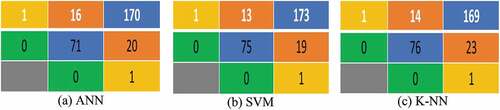
Figure 9. Performance Measures on Multiple Frequency Bands.

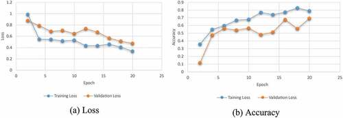
Table 4. ML Algorithm comparison using F1-score and Accuracy.

Classifier	ANN	SVM	KNN	i-YOLO v5
Accuracy	88.19	89.92	89.96	91.19
F1-score	91.11	91.06	91.18	91.26

Segmented Image Quality Measures Using McCulloch Algorithm

MSE (Mean Square Error), PSNR (Peak Signal to Noise Ratio), SSIM (Structured Similarity Index Method), FSIM (Feature Similarity Index Method), and other image quality techniques are widely used to evaluate and assess image quality. This study looked at how well the SSIM, FSIM, MSE, and PSNR methods work for accurate segmentation.

Mean Square Error (MSE)

MSE is a commonly used image quality metric. Thus, the values rounded off to zero are better as it’s a comprehensive reference metric. The MSE measures the errors’ average square. Absolute error between approximate and outcome, Equation (23)(23) $\mathrm{M}\mathrm{e}\mathrm{a}\mathrm{n}\mathrm{S}\mathrm{q}\mathrm{u}\mathrm{a}\mathrm{r}\mathrm{e}\mathrm{E}\mathrm{r}\mathrm{r}\mathrm{o}\mathrm{r}=\frac{1}{MN}\sum _{i=0}^M\sum _{j=0}^N[g(n,m)-g(m,n){]}^2$(23) . Considering the predictable squared error/quadratic loss ratio, it’s a risk function.

$g_{x,y}(.);g_{x,y}(.)$are the two images among MSE that is well-defined as

(23) $\mathrm{M}\mathrm{e}\mathrm{a}\mathrm{n}\mathrm{S}\mathrm{q}\mathrm{u}\mathrm{a}\mathrm{r}\mathrm{e}\mathrm{E}\mathrm{r}\mathrm{r}\mathrm{o}\mathrm{r}=\frac{1}{MN}\sum _{i=0}^M\sum _{j=0}^N[g(n,m)-g(m,n){]}^2$(23)

Peak Signal to Noise Ratio (PSNR)

The ratio between the maximum allowable signal power and the PSNR is calculated. And the distorting noise’s power has an impact on the quality of its portrayal. The decibel ratio between the two images is calculated. Because of the wide dynamic range of signals, the PSNR is commonly calculated as a decibel scale logarithmic term. This dynamic range ranges from the highest to the lowest possible values, which are affected by their quality. Lossy image compression codecs’ reconstruction is typically evaluated using PSNR. The error caused by compression or distortion is referred to as noise. When compared to compression codecs, PSNR approximates reconstruction quality. For 32-bit data, the PSNR is in the 45–65 dB range, while for 64-bit data, it is in the 75–95 dB range. The loss in wireless quality is 15–20 dB. The peak value refers to the highest point in the image data. 255 is the Peak Value of a 16-bit unsigned integer data type. A description of the total error in dB can be seen from Equation (24)(24) $\mathrm{P}\mathrm{e}\mathrm{a}\mathrm{k}\mathrm{S}\mathrm{i}\mathrm{g}\mathrm{n}\mathrm{a}\mathrm{l}\mathrm{t}\mathrm{o}\mathrm{N}\mathrm{o}\mathrm{i}\mathrm{s}\mathrm{e}\mathrm{R}\mathrm{a}\mathrm{t}\mathrm{i}\mathrm{o}=10\mathrm{L}\mathrm{o}{\mathrm{g}}_{10}\frac{({\mathrm{P}\mathrm{e}\mathrm{a}\mathrm{k}\mathrm{V}\mathrm{a}\mathrm{l}\mathrm{u}\mathrm{e}}_i^2)}{\mathrm{M}\mathrm{S}\mathrm{E}}$(24) .

(24) $\mathrm{P}\mathrm{e}\mathrm{a}\mathrm{k}\mathrm{S}\mathrm{i}\mathrm{g}\mathrm{n}\mathrm{a}\mathrm{l}\mathrm{t}\mathrm{o}\mathrm{N}\mathrm{o}\mathrm{i}\mathrm{s}\mathrm{e}\mathrm{R}\mathrm{a}\mathrm{t}\mathrm{i}\mathrm{o}=10\mathrm{L}\mathrm{o}{\mathrm{g}}_{10}\frac{({\mathrm{P}\mathrm{e}\mathrm{a}\mathrm{k}\mathrm{V}\mathrm{a}\mathrm{l}\mathrm{u}\mathrm{e}}_i^2)}{\mathrm{M}\mathrm{S}\mathrm{E}}$(24)

Structure Similarity Index Method (SSIM)

Image degradation is defined as a change in structural information perception in SSIM. Across these three categories, the weighted average of resemblance is the emergence of a statistic. 0.5 for edges, 0.25 for texture, and 0.25 for grayscale are proposed weights. Moreover, it should also be noted that the findings that are similar in subjective judgments are influenced by using a 1/0/0 weight measurement. It implies that the edge of image regions dominates image quality perception rather than textures (or) smooth regions. The luminance_c is 1, and the contrast is “c,” the structure is s, and the positive constants are α, β and γ (Equation (25)(25) $\mathrm{S}\mathrm{t}\mathrm{r}\mathrm{u}\mathrm{c}\mathrm{t}\mathrm{u}\mathrm{r}\mathrm{e}\mathrm{S}\mathrm{i}\mathrm{m}\mathrm{i}\mathrm{l}\mathrm{a}\mathrm{r}\mathrm{i}\mathrm{t}\mathrm{y}\mathrm{I}\mathrm{n}\mathrm{d}\mathrm{e}\mathrm{x}\mathrm{M}\mathrm{e}\mathrm{t}\mathrm{h}\mathrm{o}\mathrm{d}(x,y)=[L(x,y){]}^{\alpha }\otimes [C(x,y){]}^{\beta }\otimes [S(x,y){]}^{\lambda }$(25) ).

(25) $\mathrm{S}\mathrm{t}\mathrm{r}\mathrm{u}\mathrm{c}\mathrm{t}\mathrm{u}\mathrm{r}\mathrm{e}\mathrm{S}\mathrm{i}\mathrm{m}\mathrm{i}\mathrm{l}\mathrm{a}\mathrm{r}\mathrm{i}\mathrm{t}\mathrm{y}\mathrm{I}\mathrm{n}\mathrm{d}\mathrm{e}\mathrm{x}\mathrm{M}\mathrm{e}\mathrm{t}\mathrm{h}\mathrm{o}\mathrm{d}(x,y)=[L(x,y){]}^{\alpha }\otimes [C(x,y){]}^{\beta }\otimes [S(x,y){]}^{\lambda }$(25)

Features Similarity Index Matrix (FSIM)

FSIM compares input photos by mapping features and measures similarities. To further understand FSIM, we need to define two test case. Gradient Magnitude (GM) and Phase Congruency (PC). In this work, the similarity among input images is used to measure image quality. Let’s say the input images are TIM-1 (Actual Input Image) and TIM-II (Backlog Input Image), with PC-I and PC-II denoting phase congruency, respectively. The PC and GM maps were created using the input images TIM-1 and TIM-2. The GM-I and GM-II algorithms were also extracted from the input images. PC-I, PC-II, GM-I and GM-II, and Equation (26)(26) $S_G=\frac{2G_1{G}_2+T_2}{G_1^2+G_2^2+T_2}$(26) can all be used to define and calculate FSIM.

(26) $S_G=\frac{2G_1{G}_2+T_2}{G_1^2+G_2^2+T_2}$(26)

Wherein T2 seems to be a positive constant that relies upon this dynamic range of gradient magnitude. TIM-I and TIM-2 are kept constant in this study so that the FSIM can be employed easily (Figure 10).

Figure 10. Grid Output for Convolutional Layer Activations for Classification.

The parameters control the relative relevance of PC and GM features. For clarity, we set an equal to 1 in this paper. It is clear from Equation (27)(27) $S_l(x)=[S_{pc}(x{)}^{\alpha }\oplus S_g(x{)}^{\beta }]$(27) that FSIM is normalized (0–1). Table 5 shows quantitative results in PSNR, SSIM, FSIM, and MSE, with bands such as Low and High.

(27) $S_l(x)=[S_{pc}(x{)}^{\alpha }\oplus S_g(x{)}^{\beta }]$(27)

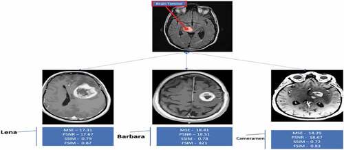
Table 5. Performance Metrics of Image Quality (MSE, PSNR, SSIM, FSIM).

Image	Noise Level	PSNR	MSE	SSIM	FSIM
Lena	0.31	22.67	22.34	0.79	0.891
	0.46	17.98	17.95	0.75	0.873
	0.67	15.21	15.24	0.71	0.812
Barbara	0.34	22.98	22.99	0.81	0.891
	0.47	18.89	18.91	0.76	0.858
	0.68	16.59	16.67	0.72	0.815
Cameramen	0.33	22.89	22.91	0.74	0.852
	0.48	19.29	19.31	0.77	0.861
	0.69	17.28	18.21	0.78	0.881

The proposed algorithms’ matrices are demonstrated in this study by tabular results, as given in Table 6.

Table 6. Performance measure of MSE, PSNR, SSIM, FSIM, CPU Time.

Images	PSNR	MSE	SSIM	FSIM	CPU Time
Img015	25.01	257.18	0.852	0.841	1.791
Img022	26.19	182.19	0.869	0.853	1.836
Img034	27.28	159.29	0.878	0.862	1.879

Optimized i-YOLOV5 CNN Models

Fivefold cross-validation is used to analyze the best model’s classifier performance. Generally, out of the fivefold dataset, four sets are predominantly used for training and the 5^th set for testing. For each fold, the task’s classification performance is assessed, and the model’s average classification is determined. The training and validation phases’ greater accuracies are futile when the trained and HPO-tuned CNNs are tested on forecasting unseen samples. To test the trained CNN’s potential to predict sample data, a test dataset is chosen randomly and divided from the training and validation datasets; otherwise, a biased dataset assessment could provide high accuracy. With a 60:20:20 ratio, already sufficient images could be classified as training, validation, and test sets randomly since the research has 500 samples, as shown in Table 7. 299 images are randomly selected from each class’s dataset and utilized for testing purposes. CNNs’ first convolutional layer could learn features such as color and edges, whilst the second convolutional layer learns the susceptible features such as BT borders. The previous convolutional layers learn the features that are combined by the following convolutional layers. In the classification task based on the first convolutional layer of CNN, there are 128 channels, 96 of which are illustrated in Figure 11. Each layer is down with 3-D array channels.

Figure 11. The performance measures of mAps of i-YOLOV5 iterations.

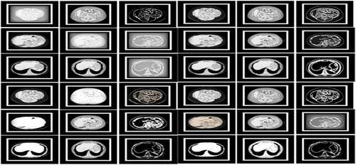
Table 7. Learning models of the CNN Models.

Classification	Type	Each Type	Training	Validation	Test
Iter_1	No Tumor	360	377	89	89
Iter_1	Tumor	240
Iter_2	Glioma	110	340	78	78
Iter_2	Meningioma	100
Iter_2	Metastatic	105
Iter_2	Normal	80
Iter_2	Pituitary	105
Iter_3	Score I	160	335	89	89
Iter_3	Score II	180
Iter_3	Score III	160

Moreover, as shown in Table 8, the performance measures like mAP and IoU are used to validate the i-YOLOV5 model, with an accomplishment of mAP of 0.98, 0.99, and 1.00 tested data sets, respectively, by the proposed method (Figure 12). Figure 13 shows the proposed plan for finding the region on the body where the tumor is most likely to be.

Figure 12. Localization Results of Input Images with Localization Values.

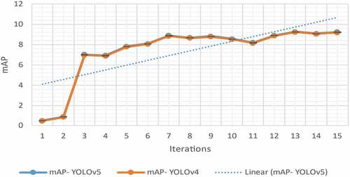
Figure 13. Loss and Accuracy graph of BT detection.

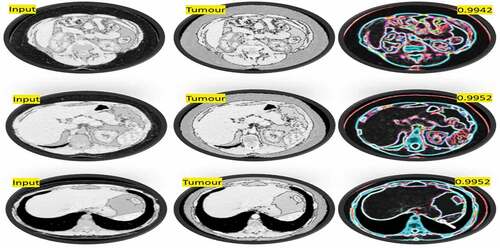
Table 8. Localization of Proposed Method.

Datasets	mAP	IoU
500	1.01	1.00

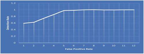
Following the classification process, the efficiency of CNN models should be evaluated using a variety of reliable approaches (Figures 14 (a) and (b)). To evaluate the models used in this work, the AUC of the ROC curve, precision metrics, specificity, accuracy, sensitivity, and precision metrics are used. The ROC curve’s AUC value is 0.9994. The BT is classified using these findings that support the proposed capacity of the i-YOLOV5 model (Figure 15).

Figure 14. ROC Curve for proposed i- YOLOV5.

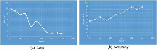
Figure 15. Confusion Matrix of BT classification using proposed model.

Table 9 for accuracy metrics using factors such as TP, TN, FP, FN, Specificity, Sensitivity, Accuracy, and Precision.

Table 9. Analysis of Accuracy metrics of TP, TN, FP, FN, Accuracy, Specificity, Sensitivity, and Precision.

Performance Measures	Classes	True Positive	True Negative	False Positive	False Negative	Accuracy (%)	Specificity	Sensitivity	Precision
Iter_1	No Tumor	271	329	5	1	99.12	0.989	0.9912	0.9891
Iter_1	Tumor	325	275	1	5	99.23	0.999	0.9891	0.9918
Iter_2	Glioma	184	600	9	10	98.28	0.9878	0.9577	0.9481
Iter_2	Meningioma	132	650	10	11	98.67	0.9867	0.9561	0.9341
Iter_2	Metastatic	139	645	7	15	98.48	0.9989	0.9182	0.9671
Iter_2	Normal	160	599	26	12	96.97	0.9718	0.9381	0.8919
Iter_2	Pituitary	129	645	11	15	97.89	0.9819	0.8919	0.9012
Iter_3	Score I	330	575	13	8	99.29	0.9839	0.9791	0.9718
Iter_3	Score II	249	675	2	1	99.991	0.9998	0.9919	0.9929
Iter_3	Score III	329	578	8	11	99.17	0.9987	0.9829	0.989

The i-YOLOV5 model’s tumor object classification with detection performance is assessed using the following evaluation matrices: Precision (P), Recall (R), F1-score (F1), and mean Average Precision (mAP) are the four components of precision. Precision refers to a model’s ability to detect only relative objects. Recall, on the other hand, refers to a model’s capacity to locate all relevant cases. Equation (28)(28) $P=\frac{N_{TP}}{N_{TP}+N_{FP}}$(28) , Equation (29)(29) $R=\frac{N_{TP}}{N_{TP}+N_{FN}}$(29) , Equation (30)(30) $F1=\frac{2\times N_{TP}}{2\times N_{TP}+N_{FN}+N_{FP})}$(30) , and Equation (31)(31) $mAP=\sum _{i=1}^{N}P(i)\times \mathrm{\Delta }R(i)$(31) are used to calculate the evaluation matrices:

(28) $P=\frac{N_{TP}}{N_{TP}+N_{FP}}$(28)

(29) $R=\frac{N_{TP}}{N_{TP}+N_{FN}}$(29)

(30) $F1=\frac{2\times N_{TP}}{2\times N_{TP}+N_{FN}+N_{FP})}$(30)

(31) $mAP=\sum _{i=1}^{N}P(i)\times \mathrm{\Delta }R(i)$(31)

where N_TP denotes the number of tumor images that were accurately identified as tumors (benign/malignant), N_FP denotes the number of images that were identified as tumor errors benign/malignant), N_FN denotes the number of images that were wrongly identified as tumors (), P(i) denotes the precision, and ΔR(i) denotes the alteration in recall from the i^th detection.

The results of the proposed CNN model are worthy of analysis in association with the established state-of-the-art CNN models (Figure 16). By utilizing the CNN models of popular and pre-trained ones such as Inceptionv3, AlexNet, GoogleNet, ResNet-50, VGG-16, and YOLO4, the same assessment was carried out (Figure 17).

Figure 16. Confusion Matrix of BT classification using proposed model.

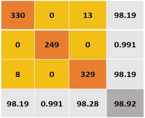
Figure 17. Performance measure of Proposed model vs other models.

Table 10 displays the utilization of these networks in obtaining the outcomes. A comparison between the proposed i-YOLOV5 models and standard YOLOV5 was made about the accuracy and AUC obtained throughout the experiments.

Table 10. Comparison of classification performance between proposed and existing state-of-the-art techniques.

Models	Classification
	Accuracy	AUC
AlexNet	88.13	0.8918
ResNet50	92.19	0.9318
Inception3	85.27	0.8819
GoogleNet	73.41	0.8129
VGG16	87.19	0.9103
Proposed i-YOLOV5	99.32	0.9918

The i-loss YOLOV5‘s functions were tested first in the experiment. Default YOLOV5‘s loss function is the Binary Cross-Entropy Loss (BC-EL). In order to achieve a higher level of performance, we investigated the following performance losses. 1. BC-EL loss plus IoU loss, 2. Focal loss plus IoU loss, 3. Focal loss plus D-IoU loss (Table 11)

Table 11. Proposed (i-YOLOV5) BT detection with different losses on test datasets.

Method	Loss_Class	Loss_Configuration	Loss_IoU	Loss_Total	mAp
BC-EL + IoU Loss	0.31023	0.68272	0.95657	2.4759	0.82812
Focal Loss + IoU Loss	0.29281	0.28278	0.76373	1.59396	0.88292
Focal Loss + D-IoU Loss	0.32918	0.70182	0.48373	2.18387	0.9024

In general, the performance is improved when a focal loss is used instead of BC-EL, as illustrated in Table 12. The mAP value in the i-YOLOV5 models was 82.812% with BC-EL+IoU loss and 88.292% with Focal+IoU loss. On test datasets, the mAP value gap had the highest value of 90.24% when Focal+D-IoU loss was used. Focal loss’s positive effects on performance in this BT detection application on test datasets are clearly shown. The proposed method has a faster rate of convergence than the conventional method. It was stated that after 10 epochs, our proposed model has a mAP of 90.24%, which is higher than the mAP of 38% for the standard i-YOLOV5 models.

Table 12. The i-YOLOV5 is compared to other models by (Bernal et al. 2019).

Model	mAP
YOLOV5 (Bernal et al. 2019)	88.28%
i-YOLOV5 (Proposed)	90.24%

The proposed model, which is proposed in this study, yielded the highest mAP value, as shown in Table 12. The original YOLOV5 was created to locate objects in landscape RGB images. It has many applications within the realm of a CV within the scope of this research work, and we applied a BT detection application to MRI scans. MRI-BT detection improved with Focal+D-IoU Loss in YOLOV5, an anchorless detector. i-YOLOV5, a supported model, and CenterNet, an effective method, have lower mAP values than this proposed model.

Conclusion and Future Work

In the field of medical image analysis, Brain Tumor identification is a crucial challenge to radiologists. As the application of DL techniques require massive amount of annotated ground truth data, it fails to implement for MR images based Brain Tumor classification. Therefore, the current research work is proposed utilizing improvised cuckoo search method for faster convergence and accurate results. For enhancement of results, the Hybrid Grid Search Optimizer Algorithm is applied to find the optimal range of each hyper parameters in which the proposed network provides accurate classification. This work investigated the appropriateness of the MSE, SSIM, FSIM, PSNR, and CPU Time approaches for segmentation accuracy. The proposed method has faster rate of convergence than the conventional counterpart search methods. It is worth to that after 10 epochs, our proposed model gained mAP of 90.24%, which is higher than the mAP of 38% for the standard i-YOLOV5 models. A comparison of proposed i-YOLOV5 models with standard YOLOV5 networks was made about the accuracy and AUC obtained throughout the experiments. Furthermore, the efficiency of testing phase is revealed by its highest accuracy value using proposed YOLOV5 model. It determines the ability of proposed model to automatically classify Brain Tumor MR images by bounding box of accurate position. Thus, the identification of Brain Tumor malignant images have been successfully implemented with accurate result. It can be concluded that the proposed algorithm holds the capability of processing large set of BT images to provide quicker outcome in medical image analysis. In future work, the improvised version of proposed YOLOV5 can support noisy BT MR images for malignant identification.

Disclosure statement

No potential conflict of interest was reported by the author(s).

References

- Anaraki, A.K., M. Ayati, and F. Kazemi. 2019. Magnetic resonance imaging-based brain tumor grades classification and grading via convolutional neural networks and genetic algorithms. Biocybernetics and Biomedical Engineering 39 (1):63–4014. doi:10.1016/j.bbe.2018.10.004.
- Apostolopoulos, I. D., and T. A. Mpesiana. 2020. COVID-19: Automatic detection from x-ray images utilizing transfer learning with convolutional neural networks. Physical and Engineering Sciences in Medicine 43 (2):1. doi:10.1007/s13246-020-00865-4.
- Azizi, S., B. Mustafa, F. Ryan, Z. Beaver, J. Freyberg, J. Deaton, A. Loh, A. Karthikesalingam, S. Kornblith, T. Chen, et al. 2021. Big self-supervised models advance medical image classification. arXiv preprint arXiv:2101 05224 eess.IV:3478–3488.
- Bahadure, N. B., A. K. Ray, and H. P. Tethi. 2017.Image analysis for MRI-based brain tumor detection and feature extraction using biologically inspired BWT and SVM. International Journal of Biomedical Imaging 2017:1–12. doi: 10.1155/2017/9749108.
- Banerjee, I., M. C. Chen, M. P. Lungren, and D. L. Rubin. 2018.Radiology report annotation using intelligent word embeddings: Applied to multi-institutional chest CT cohort. Journal of Biomedical Informatics 77:11–20. doi: 10.1016/j.jbi.2017.11.012.
- Begum, S. S., and D. R. Lakshmi. 2020. Combining optimal wavelet statistical texture and recurrent neural network for tumour detection and classification over MRI. Multimedia Tools and Applications 79:1–22.
- Benjamens, S., P. Dhunnoo, and B. Mesk´o. 2020. The state of artificial intelligence-based FDA-approved medical devices and algorithms: An online database. NPJ Digital Medicine 3 (1):1–8. doi:10.1038/s41746-020-00324-0.
- Benjdira, B., T. Khursheed, A. Koubaa, A. Ammar, and K. Ouni Car detection using unmanned aerial vehicles: Comparison between faster R-CNN and yolov3. In Proceedings of the 2019 1st International Conference on Unmanned Vehicle Systems-Oman (UVS), Muscat, Oman, 5–7 February 2019; IEEE: Muscat, Oman, 2019; vol. 79, pp. 1–6.
- Bernal, J., K. Kushibar, D. S. Asfaw, S. Valverde, A. Oliver, R. Martí, and X. Lladó. 2019.Deep convolutional neural networks for brain image analysis on magnetic resonance imaging: A review. Artificial intelligence in medicine 95:64–81. doi: 10.1016/j.artmed.2018.08.008.
- Bochkovskiy, A. 2020. Yolo v4, v3 and v2 for Windows and Linux. GitHub 2020 April https://github.com/AlexeyAB/darkne.
- Bochkovskiy, A., C.-Y. Wang, and H.-Y.M Liao. 2020. YOLOv4: Optimal speed and accuracy of object detection. arXiv 2020, arXiv:2004 10934 cs.CV. doi:10.48550/arXiv.2004.10934.
- Chenjie, G., I.-H. Gu, A.S. Jakola, and J. Yang (2018) Deep learning and multi-sensor fusion for glioma classification using multistream 2D convolutional networks. In: 2018 40th Annual International Conference of the IEEE Engineering in Medicine and Biology Society (EMBC), Honolulu, HI, USA, IEEE, pp. 5894–97.
- Chen, D., S. Liu, P. Kingsbury, S. Sohn, C. B. Storlie, E. B. Habermann, J. M. Naessens, D. W. Larson, and H. Liu. December 2019. Deep learning and alternative learning strategies for retrospective real-world clinical data. NPJ Digital Medicine 2(1):43. doi: 10.1038/s41746-019-0122-0.
- Destrempes, F., M. Mignotte, and J. F. Angers. 2005. A stochastic method for Bayesian estimation of Hidden Markov Random field models with application to a color model. IEEE Transactions on Image Processing 14 (8):1096–108. doi:10.1109/TIP.2005.851710.
- Dorrer, M., and A. Tolmacheva. 2020. Comparison of the YOLOv3 and Mask R-CNN architectures’ efficiency in the smart refrigerator’s computer vision. Journal of Physics Conference Series 1679 (4):042022. doi:10.1088/1742-6596/1679/4/042022.
- Dosovitskiy, A., L. Beyer, A. Kolesnikov, D. Weissenborn, X. Zhai, T. Unterthiner, M. Dehghani, M. Minderer, G. Heigold, S. Gelly, et al. 2020. An image is worth 16x16 words: Transformers for image recognition at scale. arXiv preprint arXiv:2010 11929. doi:10.48550/arXiv.2010.11929.
- Dosovitskiy, A., L. Beyer, A. Kolesnikov, D. Weissenborn, X. Zhai, T. Unterthiner, M. Dehghani, M. Minderer, G. Heigold, S. Gelly, et al. An image is worth 16x16 words: Transformers for image recognition at scale. In 9th International Conference on Learning Representations, ICLR 2021, Virtual Event, Austria, May 3-7 2021, 2021.
- Feng, X., N. J. Tustison, S. H. Patel, and C. H. Meyer. 2020. Brain Tumor Segmentation Using an Ensemble of 3D U-Nets and Overall Survival Prediction Using Radiomic Features. Frontiers in computational neuroscience 14:1–12. doi: 10.3389/fncom.2020.00025.
- Fu, J., X. Sun, Z. Wang, and K. Fu. 2020. An anchor-free method based on feature balancing and refinement network for multiscale ship detection in SAR images. IEEE Transactions on Geoscience and Remote Sensing 59:1331–1344.
- Ge, Z., S. Liu, F. Wang, Z. Li, and J. Sun. 2021. Yolox: Exceeding Yolo series in 2021. arXiv 2021, arXiv:2107 08430. doi:10.48550/arXiv.2107.08430.
- Ghiasi, G., T.-Y. Lin, and Q. V. Le. NAS-FPN: Learning scalable feature pyramid architecture for object detection. In Proceedings of the IEEE/CVF Conference on Computer Vision and Pattern Recognition, pages 7036–45, 2019. doi:10.48550/arXiv.1904.07392.
- He, K., X. Zhang, S. Ren, and J. Sun. 2015. Deep Residual Learning for Image Recognition. IEEE. doi:10.1109/CVPR.2016.90.
- Iqbal, S., M. U. Ghani, T. Saba, A. Rehman, and P. Saggau. 2018. Brain tumor segmentation in multi-spectral MRI using convolutional neural networks (CNN). Microscopy Research and Technique 81 (4):419–27. doi:10.1002/jemt.22994.
- Jocher, G. 2020. YOLOv5(GitHub). https://zenodo.org/record/4418161#.X_iH_ugzaUk
- Kaur, T., B. S. Saini, and S. Gupta. 2019. An adaptive fuzzy K-nearest neighbor approach for MR brain tumor image classification using parameter-free bat optimization algorithm. Multimedia Tools Appl 78 (15):1–38. doi:10.1007/s11042-019-7498-3.
- Kim, J. A., J. Y. Sung, and S. H. Park Comparison of Faster-RCNN, YOLO, and SSD for real-time vehicle type recognition. In Proceedings of the 2020 IEEE International Conference on Consumer Electronics-Asia (ICCE-Asia), Seoul, Korea, 1–3 November 2020; IEEE: Piscataway, NJ, USA, 2020; pp. 1–4.
- Liang, H., X. Sun, Y. Sun, and Y. Gao. 2017. Text feature extraction based on deep learning: A review. EURASIP Journal on Wireless Communications and Networking 2017 (1):1–12. doi:10.1186/s13638-017-0993-1.
- Liu, S., L. Qi, H. Qin, J. Shi, and J. Jia. Path aggregation network, for instance segmentation. In Proceedings of the IEEE conference on computer vision and pattern recognition, Salt Lake City, UT, USA, 2018; pp. 8759–68.
- Li, M., Z. Zhang, L. Lei, X. Wang, and X. Guo. 2020. Agricultural greenhouses detection in high-resolution satellite images based on convolutional neural networks: Comparison of Faster R-CNN, YOLOv3 and SSD. Sensors 20 (17):4938. doi:10.3390/s20174938.
- Li, L., Z. Zhou, B. Wang, L. Miao, and H. Zong. 2021. A novel CNN-based method for accurate ship detection in HR optical remote sensing images via rotated bounding box. IEEE Transactions on Geoscience and Remote Sensing 59 (1):686–99. doi:10.1109/TGRS.2020.2995477.
- Long, X., K. Deng, G. Wang, Y. Zhang, Q. Dang, Y. Gao, H. Shen, J. Ren, S. Han, and D. E. PP-YOLO. 2020. An effective and efficient implementation of object detector. arXiv 2020, arXiv:2007 12099.
- Louis, D. N., A. Perry, G. Reifenberger, A. von Deimling, D. Figarella-Branger, W. K. Cavenee, H. Ohgaki, O. D. Wiestler, P. Kleihues, and D. W. Ellison. 2016. The 2016 World Health Organization classification of tumors of the central nervous system: A summary. Acta neuropathologica 131 (6):803–20. doi:10.1007/s00401-016-1545-1.
- Malarvel, M., G. Sethumadhavan, P. C. Rao Bhagi, S. Kar, T. Saravanan, and A. Krishnan. 2017. Anisotropic diffusion based denoising on X-radiography images to detect weld defects. Digital signal processing 68:112–26. doi: 10.1016/j.dsp.2017.05.014.
- Mårtensson, G., D. Ferreira, T. Granberg, L. Cavallin, K. Oppedal, A. Padovani, I. Rektorova, L. Bonanni, M. Pardini, and M. G. Kramberger. 2020. The reliability of a deep learning model in clinical out-of-distribution MRI data: A multicohort study. Medical Image Analysis 66:101714. Publisher: Elsevier. doi:10.1016/j.media.2020.101714.
- Menze, B. H., J. Andras, B. Stefan, et al. 2015. The Multimodal Brain Tumor Image Segmentation Benchmark (BRATS). IEEE Transactions on Medical Imaging. 34(10):1993–2024. doi:10.1109/TMI.2014.2377694.
- Mitani, A., A. Huang, S. Venugopalan, G. S. Corrado, L. Peng, D. R. Webster, N. Hammel, Y. Liu, and A. V. Varadarajan. Jan 2020. Detection of anaemia from retinal fundus images via deep learning. Nature Biomedical Engineering 4(1):18–27. doi: 10.1038/s41551-019-0487-z.
- Narmatha, C., S.M. Eljack, T. AARM, S. Manimurugan, and M. Mustafa. 2020. A hybrid fuzzy brain- storm optimization algorithm for the classification of brain tumor MRI images. Journal of Ambient Intelligence and Humanized Computing. doi:10.1007/s12652-020-02470-5.
- Pan, Y., W. Huang, Z. Lin, W. Zhu, J. Zhou, J. Wong, and Z. Ding. “Brain tumor grading based on neural networks and convolutional neural networks.” 2015 37th Annual International Conference of the IEEE Engineering in Medicine and Biology Society (EMBC). Milan, Italy: IEEE, 2015.
- Pei, L., S. Bakas, A. Vossoughe, M. S. R. Syed, C. Davatzikos, and K. M. Iftekharuddin. 2020. Longitudinal brain tumor segmentation prediction in MRI using feature and label fusion. Biomedical signal processing and control 55:101648. doi:10.1016/j.bspc.2019.101648.
- Pei, L., L. Vidyaratne, M. Monibor Rahman, and K. M. Iftekharuddin. 2020. Deep learning with context encoding for semantic brain tumor segmentation and patient survival prediction. In Medical Imaging 2020: Computer-Aided Diagnosis. vol. 11314, pp. 113140H. International Society for Optics and Photonics. doi:10.1117/12.2550693.
- Philip Bachman, R. D. H., and W. Buchwalter. 2019. Learning representations by maximizing mutual information across views. Advances in Neural Information Processing Systems 15535–45. https://doi.org/10.48550/arXiv.1906.00910
- Rahman, E. U., Y. Zhang, S. Ahmad, H. I. Ahmad, and S. Jobaer. 2021. Autonomous vision-based primary distribution systems porcelain insulators inspection using UAVs. Sensors 21 (3):974. doi:10.3390/s21030974.
- Shukla, G., G. S. Alexander, S. Bakas, R. Nikam, K. Talekar, J. D. Palmer, and W. Shi. 2017. Advanced magnetic resonance imaging in glioblastoma: A review. Chinese Clinical Oncology 6 (4):1–12. doi:10.21037/cco.2017.06.28.
- Solawetz, J. 2020. YOLOv5 New Version - Improvements and Evaluation. Roboflow. https://blog.roboflow.com/yolov5-improvements-and-evaluation/.
- Van Leemput, K., F. Maes, D. Vandermeulen, A. Colchester, and P. Suetens. 2001. Alan Colchester and Paul Suetens. Automated segmentation of multiple sclerosis lesions by model outlier detection. IEEE Transactions on Medical Imaging 20 (8):677–88. doi:10.1109/42.938237.
- Wang, C.-Y., I.H.Y Hong-Yuan Mark Liao, W. Yueh-Hua, P.-Y. Chen, and J.-W. Hsieh. 2019. CSP-NET: A new backbone that can enhance learning capability of CNN. arXiv. https://arxiv.org/pdf/1911.11929.pdf.
- Wiesmüller, S., and D. A. Chandy. (2010). Content-based mammogram retrieval using Gray level matrix. In Proceedings of the International Joint Journal Conference on Engineering and Technology (IJJCET 2010), Chennai, India, pp. 217–21.
- Yu, Z., Y. Shen, and C. Shen. 2021. A real-time detection approach for bridge cracks based on YOLOv4-FPM. Automation in Construction 122: 103514. doi:10.1016/j.autcon.2020.103514.
- Zhao, K., and X. Ren Small aircraft detection in remote sensing images based on YOLOv3. In Proceedings of the IOP Conference Series: Materials Science and Engineering, Guangzhou, China, 12–14 January 2019.