Deep Learning Based Object Attitude Estimation for a Laser Beam Control Research Testbed

ABSTRACT

This paper presents an object attitude estimation method using a 2D object image for a Laser Beam Control Research Testbed (LBCRT). Motivated by emerging Deep Learning (DL) techniques, a DL model that can estimate the attitude of a rotating object represented by Euler angles is developed. Instead of synthetic data for training and validation of the model, customized data is experimentally created using the laboratory testbed developed at the Naval Postgraduate School. The data consists of Short Wave Infra-Red (SWIR) images of a 3D-printed Unmanned Aerial Vehicle (UAV) model with varying attitudes and associated Euler angle labels. In the testbed, the estimated attitude is used to aim a laser beam to a specific point of the rotating model UAV object. The attitude estimation model is trained with 1684 UAV images and validated with 421 UAV images not used in the model training. The validation results show the Root-Mean-Square (RMS) angle estimation errors of 6.51 degrees in pitch, 2.74 degrees in roll, and 2.51 degrees in yaw. The Extended Kalman Filter (EKF) is also integrated to show the reduced RMS estimation errors of 1.36 degrees in pitch, 1.20 degrees in roll, and 1.52 degrees in yaw.

Introduction

Attitude estimation of a rotating object from a 2D object image eliminates the need for a dedicated attitude estimation sensor and allows remote determination of object attitude. Image-based attitude estimation has been studied in many different applications. Pose (position and attitude) estimation based on DL has been considered for airplanes in airports to prevent collisions (Fu et al. 2019). DL Image-based attitude estimation can be used in spacecraft to achieve on-orbit proximity operations such as rendezvous, docking, orbital debris removal, and close-proximity formation flying missions (Phisannupawong et al. 2020; Proenc¸a 2020; Sharma, Beierle, and D’Amico 2018). For high-energy laser systems, precision laser beam pointing is a crucial technology where a laser beam control system is employed to steer the laser beam at a certain point of a maneuvering object and maintain the aim-point until the object is incapacitated.

Conventional methods of aim-point selection and maintenance require an operator to identify the object aim-point using joysticks or other instruments, steer the laser beam to this aim-point, and maintain it. This method is not practical for fast-moving objects, as every second counts when one or many objects are inbound. DL algorithms can improve reaction time to simultaneously engage fast-moving objects and multiple objects. To this end, the object’s attitude is critical information as it allows us to remotely and instantaneously determine an aim-point.

Pose estimation using DL approaches is usually divided into direct pose estimation (Mahendran et al. 2018) and geometry-based pose estimation (Chen et al. 2022; Pavlakos et al. 2017). In the former, a Convolutional Neural Network (CNN) is typically trained under a supervised learning environment to minimize the object’s pose error and predict additional unknown object poses. In the latter, two steps are employed 1) key-points predictions in the 2D image plane by architectures such as Key-points R-CNN (He et al. 2017), Hourglass (Newell, Yang, and Deng 2016), and HRNET (Sun et al. 2019), 2) optimal pose solution from the 3D and 2D objects key-points complying with the projection rules among the two sets of points. In this step, the Perspective-n-Points (PnP) algorithm is a standard solution for the optimal pose. However, new techniques such as End-to-End probabilistic pose estimation (Chen et al. 2022) have also been applied.

Motivated by the promising results of DL methods, the present investigation uses direct pose estimation approach to develop an accurate image-based attitude estimation model of a laser beam control system. The presented work focuses on several areas. As DL does not come without limitations, one of the main challenges is the limited amount of data for the training and validation process of the model development. In this paper, we first present an experimental generation of data for the training and validation of a DL model. Next, the development and performance of the DL attitude estimation model using Euler angles are presented. We also show that including extended Kalman Filter techniques in the DL model can improve the attitude estimation performance for the laser beam control application.

Experimental Data Generation

The Naval Postgraduate School has LBCRT, as shown in Figure 1. The LBCRT employs a video tracking system that uses a gimballed telescope to image a far-field target using a SWIR sensor. The SWIR track sensor and a fast steering mirror in the optical beam path are used to maintain the line-of-sight to the center of the target in a high-speed closed-loop control setting. The LBCRT requires additional operator input to steer the laser beam to a specific aim-point of a target within the tracker screen as the target undergoes pose changes.

Figure 1. Data generation experimental setup.

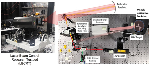
The laboratory target range is developed as shown in Figure 1 to provide image data generation capabilities. The rotational motion of the target is recreated to be as realistic as possible with a 3D-printed titanium UAV model attached to a rotational stage. The scaled UAV model has a painted surface with a wingspan of 3 inches (see Figure 2). The gimbal stepper motor’s positions are controlled to create different UAV rotational configurations, and the SWIR sensor is used to grab all the different attitude configurations of the UAV. Every data generated corresponds to an image of a UAV object with a particular attitude and corresponding labels represented by Euler angles. The procedure for generating the data is as follows:

Figure 2. 3D-printed and painted titanium UAV model.

• From MATLAB, the angular positions of the three stepper motors in the gimbal are controlled. Arduino UNO and two Adafruit Motor Shield V2 interfaces between MATLAB and motors, Arduino UNO is the controller, and Adafruit Motor Shield V2 is the driver. Figure 3 shows a detailed view of the gimbal. The stepper motors are set to micro-stepping to have a smoother motion and higher resolution, M${ }_1$ to 88.88 steps per degree, M${ }_2$ to 35 steps per degree, and M${ }_3$ to 44.44 steps per degree.

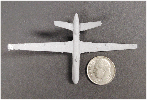
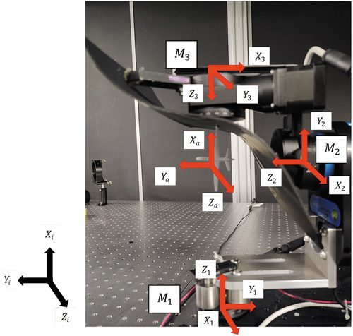
Figure 3. UAV attached to the gimbal.

• The motors respond to specific position commands, and consequently, the UAV acquires a new attitude. The UAV should generate rotational motion by placing its geometrical center at the intersection of the three motors’ rotation axes. However, as the UAV is placed by hand in the gimbal, a slight UAV offset is unavoidable. The offset creates small displacements in the UAV for each acquired attitude. The offset can be estimated by analyzing a reasonable amount of data collected and therefore compensated.

• The UAV, with the newly acquired attitude, is the input of an optical system. This system outputs a realistic UAV-size image some kilometers from the LBCRT system.

• The output of the optical system, the UAV image, is captured by the LBCRT telescope and measured by an IR camera. As the data collection process is carried out without light but light illuminating the UAV, the IR camera can measure the UAV reflectively. The black velvet background in the gimbal is to absorb any remaining light around the UAV.

• Finally, the UAV image measured by the IR camera is saved in the computer in PNG format.

Repeating the previous steps is how the data set is generated. So far, the angular reference positions are the labels, and the images are the inputs for the DL model. However, our interest is in object attitude labels instead of the motor’s angular positions.

To determine the UAV attitude from the angular reference positions, an inertial frame ($X_i,Y_i,Z_i$) is defined, and also additional frames attached to the three motors and the UAV, see Figure 3. Note that $Z_1,Z_2,Z_3$ are respectively the rotation axes of the motors $M_1,M_2,M_3$. Ideally, the axes intersect the geometrical center of the UAV. First, the rotation matrix describing the attitude of the frame ($X_1,Y_1,Z_1$) with respect to the inertial frame is calculated as (1). The rotation matrix describing the attitude of the frame ($X_2,Y_2,Z_2$) with respect the frame ($X_1,Y_1,Z_1$) is calculated as (2). The rotation matrix describing the attitude of the frame ($X_3,Y_3,Z_3$) with respect the frame ($X_2,Y_2,Z_2$) is calculated as (3). Finally, the rotation matrix describing the attitude of the frame ($X_a,Y_a,Z_a$) attached to the UAV with respect to the inertial frame ($X_3,Y_3,Z_3$) is calculated as (4). These matrices are defined below, where ${\alpha }_1,{\alpha }_2,{\alpha }_3$ are the motors’ angular positions about $Z_1,Z_2,Z_3$ respectively. These positions are positive when the motors are rotated according to the right-hand rule.

(1) $F_1=\left[\begin{array}{ccc}0& \mathrm{c}\mathrm{o}\mathrm{s}(90+{\alpha }_1)& \mathrm{c}\mathrm{o}\mathrm{s}({\alpha }_1)\\ 0& \mathrm{c}\mathrm{o}\mathrm{s}(180+{\alpha }_1)& \mathrm{c}\mathrm{o}\mathrm{s}(90+{\alpha }_1)\\ 1& 0& 0\end{array}\right]$(1)

(2) $F_2=\left[\begin{array}{ccc}\mathrm{c}\mathrm{o}\mathrm{s}({\alpha }_2)& 0& \mathrm{c}\mathrm{o}\mathrm{s}(90-{\alpha }_2)\\ \mathrm{c}\mathrm{o}\mathrm{s}(90+{\alpha }_2)& 0& \mathrm{c}\mathrm{o}\mathrm{s}({\alpha }_2)\\ 0& -1& 0\end{array}\right]$(2)

(3) $F_3=\left[\begin{array}{ccc}\mathrm{c}\mathrm{o}\mathrm{s}(90-{\alpha }_3)& 0& \mathrm{c}\mathrm{o}\mathrm{s}(180-{\alpha }_3)\\ \mathrm{c}\mathrm{o}\mathrm{s}({\alpha }_3)& 0& \mathrm{c}\mathrm{o}\mathrm{s}(90-{\alpha }_3)\\ 0& -1& 0\end{array}\right]$(3)

(4) $F_a=\left[\begin{array}{ccc}0& 0& -1\\ -1& 0& 0\\ 0& 1& 0\end{array}\right]$(4)

The rotation matrix describing the UAV attitude with respect to the inertial frame is easily computed as the matrix product

(5) $F=F_a{F}_3{F}_2{F}_1$(5)

To obtain Euler angles describing the UAV attitude with respect to the inertial frame, the previous matrix is matched to the rotation matrix dependent on Euler angles (sequence pitch ($p$), roll ($r$), and yaw($y$)), i.e.

(6) $F=\left[\begin{array}{ccc}{\mathrm{c}}_y{\mathrm{c}}_r& {\mathrm{c}}_y{\mathrm{s}}_r{\mathrm{s}}_p+{\mathrm{s}}_y{\mathrm{c}}_p& -{\mathrm{c}}_y{\mathrm{s}}_r{\mathrm{c}}_p+{\mathrm{s}}_y{\mathrm{s}}_p\\ -{\mathrm{s}}_y{\mathrm{c}}_r& -{\mathrm{s}}_y{\mathrm{s}}_r{\mathrm{s}}_p+{\mathrm{c}}_y{\mathrm{c}}_p& -{\mathrm{s}}_y{\mathrm{s}}_r{\mathrm{c}}_p+{\mathrm{c}}_y{\mathrm{s}}_p\\ {\mathrm{s}}_r& -{\mathrm{c}}_r{\mathrm{s}}_p& {\mathrm{c}}_r{\mathrm{c}}_p\end{array}\right]$(6)

where ${\mathrm{c}}_p=\mathrm{c}\mathrm{o}\mathrm{s}(p)$, ${\mathrm{c}}_y=\mathrm{c}\mathrm{o}\mathrm{s}(y)$, ${\mathrm{c}}_r=\mathrm{c}\mathrm{o}\mathrm{s}(r)$, ${\mathrm{s}}_p=\mathrm{s}\mathrm{i}\mathrm{n}(p)$, ${\mathrm{s}}_y=\mathrm{s}\mathrm{i}\mathrm{n}(y)$, ${\mathrm{s}}_r=\mathrm{s}\mathrm{i}\mathrm{n}(r)$. The Euler angles can be straightforward calculated from the previous matrices through the next relations

(7) $\frac{F_{32}}{F_{33}}=\frac{-{\mathrm{c}}_r{\mathrm{s}}_p}{{\mathrm{c}}_r{\mathrm{c}}_p}=-\mathrm{t}\mathrm{a}\mathrm{n}(p),\frac{F_{21}}{F_{11}}=\frac{-{\mathrm{s}}_y{\mathrm{c}}_r}{{\mathrm{c}}_y{\mathrm{c}}_r}=-\mathrm{t}\mathrm{a}\mathrm{n}(y),F_{31}={\mathrm{s}}_r$(7)

Where finally, these angles result as pitch, roll, and yaw respectively

(8) $p=-\mathrm{t}\mathrm{a}{\mathrm{n}}^{-1}(\frac{F_{32}}{F_{33}}),r=\mathrm{s}\mathrm{i}{\mathrm{n}}^{-1}(F_{31}),y=-\mathrm{t}\mathrm{a}{\mathrm{n}}^{-1}(\frac{F_{21}}{F_{11}})$(8)

They describe the object’s attitude with respect to the inertial frame, following the sequence pitch, roll, and yaw. We refer the reader to Kim (2013) for rigid body attitude parametrizations and transformations among them.

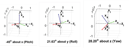
A sample of the data generated is shown on the right side of Figure 4. It consists of Euler angles labeled according to the defined sequence and of a UAV image attitude. The Euler angles label is obtained from the motors reference positions ${\alpha }_1={10}^o,{\alpha }_2={35}^o,{\alpha }_3={50}^o$ through relations (6)-(8). On the left side, this Figure also shows the reference configuration for all the generated data. The Euler angles sequence to go from the reference configuration to the sample configuration is shown in Figure 5. Starting from the reference configuration, the UAV is first rotated $-{45}^o$ about $X_a$ axis (is pitching), then it is rotated ${21.63}^o$ about $Y_a$ axis (is rolling), and finally, it is rotated ${28.20}^o$ about $Z_a$ axis (yawing).

Figure 4. Reference configuration with nose pointing to the reader (left). Example of one image collected with label $p=-{45}^o,r={21.63}^o,y={28.2}^o$ (right).

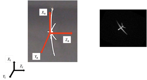
Figure 5. Euler angle sequence.

The final objective of DL attitude estimation is automatic aim-point selection. Let us assume that the point of interest is the UAV nose. From object attitude information, the aim-point can be calculated through the following relation

(9) $\left[\begin{array}{c}X{n}_i\\ Y{n}_i\\ Z{n}_i\end{array}\right]={\left[\begin{array}{ccc}{\mathrm{c}}_y{\mathrm{c}}_r& {\mathrm{c}}_y{\mathrm{s}}_r{\mathrm{s}}_p+{\mathrm{s}}_y{\mathrm{c}}_p& -{\mathrm{c}}_y{\mathrm{s}}_r{\mathrm{c}}_p+{\mathrm{s}}_y{\mathrm{s}}_p\\ -{\mathrm{s}}_y{\mathrm{c}}_r& -{\mathrm{s}}_y{\mathrm{s}}_r{\mathrm{s}}_p+{\mathrm{c}}_y{\mathrm{c}}_p& -{\mathrm{s}}_y{\mathrm{s}}_r{\mathrm{c}}_p+{\mathrm{c}}_y{\mathrm{s}}_p\\ {\mathrm{s}}_r& -{\mathrm{c}}_r{\mathrm{s}}_p& {\mathrm{c}}_r{\mathrm{c}}_p\end{array}\right]}^{\mathrm{T}}\left[\begin{array}{c}0\\ n\\ 0\end{array}\right]$(9)

where $[0n0{]}^{\mathrm{T}}$ are the UAV nose coordinates in the UAV frame ($X_a,Y_a,Z_a$), and $[X{n}_{i}Y{n}_{i}Z{n}_i{]}^{\mathrm{T}}$ are the UAV nose coordinates in the inertial frame ($X_i,Y_i,Z_i$). Here, attitude information is of paramount interest as it makes the relation (9) feasible. The matrix in 9 is the transpose of $F$ in 6 and depends on Euler angle information. The nose coordinates are in pixels. Two samples showing an aim-point selection from UAV attitude are in Figure 6.

Figure 6. Automatic aim-point selection from attitude information.

Object Attitude Estimation via Deep Learning

An attitude estimation model for the present application can be developed with the data generated from the experiment shown in the previous section. As attitude is represented in terms of Euler angles, three coefficients describing attitude, the DL problem becomes a regression problem where the output of the DL model is a set of coefficients for the corresponding attitude. Deep neural networks using CNN architecture are commonly used for imagery data analysis applications such as object detection, classification, and the regression problem considered in this paper. CNN includes the feature learning network employing three main types of operation on the input data: convolution, rectified linear unit (ReLU) as an activation function, and pooling. The extracted feature maps are used in the regression network to predict the output, which is the estimated attitude. Figure 7 shows a typical CNN architecture, where the components of the feature learning and classification (regression in our case) are detailed.

Figure 7. CNN generic architecture, (MathWorks n.d.).

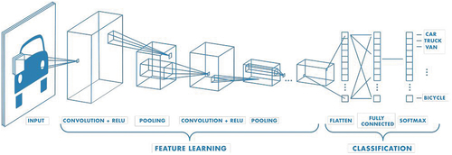
To handle the degradation of the training and validation accuracy associated with deep neural networks with a large number of layers, Resnet architecture (He et al. 2016) is employed as a DL model, which includes a shortcut through every two or more layers to allow the optimal solution to pass down through. This prevents the degrading of training and validation, where an increase of layers causes degrading in training and, consequently, in validation. Instead of training Resnet from scratch for the attitude sensing problem, pre-trained Resnet 18 architecture from the Deep Network Designer app of MATLAB software, which allows for the powerful transfer learning technique’s advantages, is used as a backbone of the DL attitude sensing model.

Resnet 18, pre-trained on the ImageNet data set, was selected to subsequently apply for the transfer learning technique on our data set. As the pre-trained architecture was trained on 1000 classes for a classification task, we replaced the last fully connected layer with 1000 neurons with a fully connected layer with just three neurons associated with the three Euler angles. In addition, the softmax and classification layers were also replaced by a regression layer to adapt the classification task to regression. Once the adaptations were made, transfer learning was applied, where the weights in the backbone were frozen. In contrast, the ones connected to the three nodes of the fully connected layer were trained on our data set to build the attitude estimation DL model.

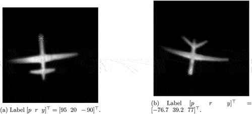
The data set consists of 1684 training images of $224\times 224\times 3$ pixels with their associated attitude labels, and 421 validation images of the same size $224\times 224\times 3$ pixels with their associated attitude labels as well. 80% of the data are for training and 20% for validation. Two samples of the data set are shown in Figure 8; every data consists of a UAV image and attitude label.

Figure 8. Two samples from the data set.

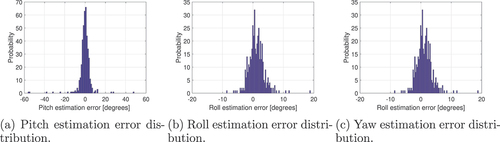
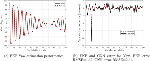
After training, the model’s performance is verified through the validation data set. Estimated attitudes produced by the CNN are compared with the real validation data. Figures 9a, 10a and 11a show both the estimated Euler angles produced by the CNN and the real Euler validation angles. Figures 9b, 10b and 11b show the CNN estimation errors defined as real minus estimated. For a good graphical illustration, just 100 data out of the 421 are considered in the Figures. The estimation error RMSEs over all the 421 validation data are 6.51 in pitch, 2.74 in roll, and 2.51 in yaw. We argue that the estimation performance can be improved by training the CNN with more than the 1684 data employed in this experiment; however, it is left for future investigation. An additional tool that is strongly effective in improving the estimation is the EKF; it is motivated because the estimation errors in Figures 9b, 10b and 11b are close to Gaussian distributions, Figure 12. The following section presents the EKF to improve the attitude estimation.

Figure 9. Pitch angle estimation.

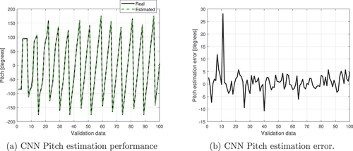
Figure 10. Roll angle estimation.

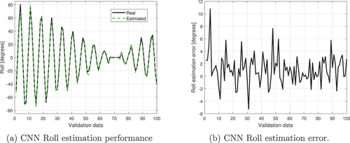
Figure 11. Yaw angle estimation.

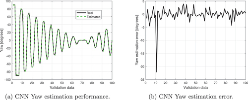
Figure 12. Attitude estimation errors distributions.

EKF as a Tool for Improving CNN Attitude Estimation

To define the EKF, a system model and a measurement are first defined; the model is defined as the Euler angles kinematics discretized by the Euler method (respecting the sequence pitch, roll, and yaw). This model defines the Euler angles evolution and is given as follows (see (Kim 2013) for details)

(10) $\underset{x_k}{\underbrace{\left[\begin{array}{c}{p}_k\\ r_k\\ y_k\end{array}\right]}}=\underset{f(x_{x-1},{\omega }_{k-1})}{\underbrace{\left[\begin{array}{c}{p}_{k-1}\\ r_{k-1}\\ y_{k-1}\end{array}\right]+\frac{1}{{\mathrm{c}}_{r_{k-1}}}\left[\begin{array}{ccc}{\mathrm{c}}_{y_{k-1}}& -{\mathrm{s}}_{y_{k-1}}& 0\\ {\mathrm{s}}_{y_{k-1}}{\mathrm{c}}_{r_{k-1}}& {\mathrm{c}}_{y_{k-1}}{\mathrm{c}}_{r_{k-1}}& 0\\ -{\mathrm{s}}_{r_{k-1}}{\mathrm{c}}_{y_{k-1}}& {\mathrm{s}}_{y_{k-1}}{\mathrm{s}}_{r_{k-1}}& {\mathrm{c}}_{r_{k-1}}\end{array}\right]\left[\begin{array}{c}{\omega }_{x_{k-1}}\\ {\omega }_{y_{k-1}}\\ {\omega }_{z_{k-1}}\end{array}\right]\mathrm{\Delta }t}}+\underset{W_{k-1}}{\underbrace{\left[\begin{array}{c}{W}_{1_{k-1}}\\ W_{2_{k-1}}\\ W_{3_{k-1}}\end{array}\right]}},$(10)

where ${\mathrm{c}}_{y_{k-1}}=\mathrm{c}\mathrm{o}\mathrm{s}(y_{k-1})$, ${\mathrm{c}}_{r_{k-1}}=\mathrm{c}\mathrm{o}\mathrm{s}(r_{k-1})$, ${\mathrm{s}}_{y_{k-1}}=\mathrm{s}\mathrm{i}\mathrm{n}(y_{k-1})$, ${\mathrm{s}}_{r_{k-1}}=\mathrm{s}\mathrm{i}\mathrm{n}(r_{k-1})$, $x_k=[p_k{r}_k{y}_k{]}^{\mathrm{T}}$ is the state vector, ${\omega }_{k-1}=[{\omega }_{x_{k-1}}{\omega }_{y_{k-1}}{\omega }_{z_{k-1}}{]}^{\mathrm{T}}$ the vector of angular velocity produced by the UAV, $W_{k-1}=[W_{1_{k-1}}{W}_{2_{k-1}}{W}_{3_{k-1}}{]}^{\mathrm{T}}$ the vector of white Gaussian noise uncertainties, finally, the parameter $\mathrm{\Delta }t=0.01$ seconds is the time consumed from $k$ to $k+1$. The measurement for the EKF is that coming from the CNN estimation described by

(11) $y_k=\underset{h(x_k)}{\underbrace{\left[\begin{array}{c}{p}_k\\ r_k\\ y_k\end{array}\right]}}+\underset{v_k}{\underbrace{\left[\begin{array}{c}{v}_{1_k}\\ v_{2_k}\\ v_{3_k}\end{array}\right]}},$(11)

where $v_k=[v_{1_k}{v}_{2_k}{v}_{3_k}{]}^{\mathrm{T}}$ is a vector of white Gaussian noise uncertainties affecting this measurement and representing the deviations shown in Figures 9b, 10b and 11b. In the above relations $W_{k-1}$ and $v_k$ are assumed to be normally distributed as $\mathcal{N}(0,Q_{k-1})$ and $\mathcal{N}(0,R_k)$ respectively, where $Q_{k-1}=1\times {10}^{-4}{I}_{3\times 3}$ is the system model noise covariance matrix, and $R_k=\mathrm{d}\mathrm{i}\mathrm{a}\mathrm{g}(0.0129,0.0019,0.0019)$ the covariance matrix of the noise affecting the measurement.

The EKF is a recursive algorithm that estimates the state vector of a nonlinear system; it is a generalization of the well-known Kalman Filter (KF) (Kalman 1960) but is dedicated to nonlinear systems. It is due to Stanley F. Schmidt and his staff (McGee et al. 1985). It keeps, although locally, the optimality property of the KF, which is the minimization of the trace of the estimation error covariance ($\mathrm{t}\mathrm{r}\mathrm{a}\mathrm{c}\mathrm{e}(E[(x_k-{\hat{x}}_k^u)(x_k-{\hat{x}}_k^u{)}^{\mathrm{T}}])$) during the estimation process. To estimate the state vector, the EKF employs the knowledge of the nonlinear system model (10) and the measurement (11). This algorithm can be found in many works of literature, see (Grewal & Andrews, 2014; Kim 2011; Simon 2006) to name a few, and is given by the following relations

(12) $\hat{x}{}_k^p=f(\hat{x}{}_{k-1}^u,{\omega }_{k-1}),$(12)

(13) $P{}_k^p=A_{k-1}{P}_{k-1}^u{A}_{k-1}^{\mathrm{T}}+Q_{k-1},$(13)

(14) $K_k=P{}_k^p{C}_k^{\mathrm{T}}(C_k{P}_k^p{C}_k^{\mathrm{T}}+R_k{)}^{-1},$(14)

(15) ${\hat{x}}_k^u=\hat{x}{}_k^p+K_k(y_k-h(\hat{x}{}_k^p)),$(15)

(16) $P_k^u=(I-K_k{C}_k)P{}_k^p,$(16)

where, $\hat{x}{}_k^p$ is the estimation of the true state before $y_k$ comes into play, $P{}_k^p$ is the predicted covariance matrix of the estimation error, $K_k$ is the Kalman gain, ${\hat{x}}_k^u$ is the optimal estimation of the true state once $y_k$ is available, and $P_k^u$ is the updated covariance matrix of the estimation error. The matrices

(17) $A_{k-1}=\frac{\mathrm{\partial }f(x_{k-1},{\omega }_{k-1})}{\mathrm{\partial }{x}_{k-1}}{|}_{\hat{x}{}_{k-1}^u},C_k=\frac{\mathrm{\partial }h(x_k)}{\mathrm{\partial }{x}_k}{|}_{\hat{x}{}_k^p}$(17)

come from the Taylor’s linear approximations of (10) and (11) around the nominal values $x_{k-1}={\hat{x}}_{k-1}^u$, $x_k={\hat{x}}_k^p$, and $W_{k-1}=v_k=0$ (see (Simon 2006)). The initial conditions employed for the EKF are $P_0^u=0.01I_{3\times 3}$, and ${\hat{x}}_0^u=[-85-5090{]}^{\mathrm{T}}$.

Figures 13a, 14a and 15a show the real Euler validation angles vs. the filtered, whereas Figures 13b, 14b and 15b show the EKF estimation errors vs. the CNN estimation errors. For illustrative purposes, only 100 of 421 data are plotted; however, the RMSEs are calculated over the 421 validation data. From Figures 13b, 14b and 15b is concluded that the EKF improves the attitude estimation performance.

Figure 13. Pitch angle estimation.

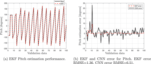
Figure 14. Roll angle estimation.

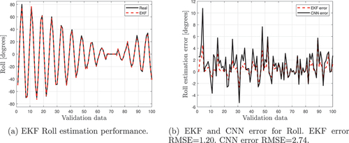
Figure 15. Yaw angle estimation.

Discussion

Image-based attitude estimation is critical in LBCRT-like systems for automatic aim-point selection. Such information solves for the aim-point selection in fast-moving objects and multiple simultaneous objects, a problem complex to solve by a human operator. In this paper, the attitude was estimated by a DL model trained on the experimental data set created in the laboratory.

Unlike many works where synthetic data are employed for the training and validation of DL models, experimental data representative for our project were created with the presented testbed. The SWIR UAV images were labeled with Euler angles for a supervised learning environment. This procedure is not straightforward as such labels are not directly available in the current testbed and were deduced from the gimbal’s motor positions via a transformation matrix. A procedure similar to forward-kinematics from robotics was applied to deduce such information. In this context, the motors played the role of joints and the UAV of the end effector.

Our DL model was trained and validated with the created data under the supervised learning environment. In the validation stage, 421 unseen data were used to deduce the quantitative and qualitative results reported in Figures 9b, 10b. Such results are reasonable for our application as they are close to the ground truth. In addition, the EKF was integrated for an improvement in the estimations. Different from traditional techniques, where training and/or CNN parameters are adjusted until a good model is yielded (e.g. (Cardoza et al. 2022; Liao et al. 2022)), the EKF was integrated as an extrinsic algorithm to improve for the estimations. The EKF combines the information predicted by the CNN with the prediction from the rotational kinematics defined in this algorithm. Such a filter generates an optimal attitude estimation outperforming CNN estimation. Figures 13b, 14b and 15b confirm the improvement.

The results are based on our current laboratory setup and require generalization and cross-validation with a more representative dataset. The paper intends to provide the general framework for collecting laboratory datasets and use a DL attitude estimation model for target tracking of a laser beam control system. An augmented data set where UAV images are corrupted with optical turbulence is considered for future work to generalize the DL models against this uncertain condition.

Conclusions

Object attitude estimation through a DL model was presented for the accurate laser object aim-pointing problem. Training and validation data were experimentally generated in the laboratory. Experimental results showed that estimated attitude in terms of Euler angles produces better performance for yaw, then for roll, and finally for pitch. Due to the Gaussian distribution of the CNN attitude estimation error, the EKF was motivated and integrated to improve the estimation performance. Training with synthetic data and validation with real LBCRT data, as well as the extension to multi-object attitude estimation, are considered for future work.

Disclosure statement

No potential conflict of interest was reported by the author(s).

Appendix

The training of our DL model was carried out in an Nvidia DGX machine with training parameters shown in Table A1. Figures A1, A2, and A3 show the architecture of the model Resnet 18 trained on our UAVs data set. Name, Type, Activation, and Learnable columns indicate the name given to each component, the type of each component, the activation means the output size of each component, and learnables the number of parameters to train at each component, respectively. It is shown that the first layer (row 1) consists of the input with size $224\times 224\times 3$ pixel, which is the size of our imagery data set. The last fully connected layer (row 69) corresponds to the 3 Euler angles with size $1\times 1\times 3$.

short-legendFigure A1.

short-legendFigure A2.

short-legendFigure A3.

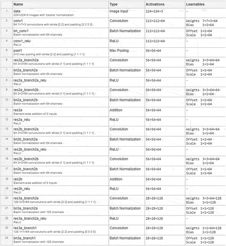
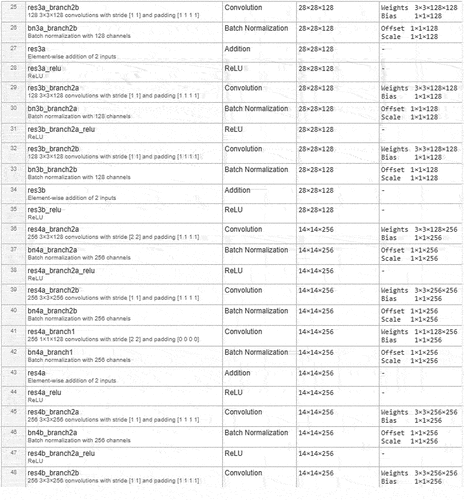
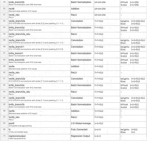
Table A1. Training parameters.

Description	Value
Learning Rate	$0.0001$
Mini Batch Size	128
Optimizer	SGDM
Epochs	$600$
$L_2$ Regularization	$0.01$
Momentum	$0.9$

References

- Cardoza, I., J. P. García-Vázquez, A. Díaz-Ramírez, and V. Quintero-Rosas. 2022. Convolutional neural networks hyperparameter tunning for classifying firearms on images. Applied Artificial Intelligence 36:1–39. doi:10.1080/08839514.2022.2058165.
- Chen, H., P. Wang, F. Wang, W. Tian, L. Xiong, and H. Li. 2022. Epro-PnP: Generalized end-to-end probabilistic perspective-n-points for monocular object pose estimation. In Proceedings of the IEEE/CVF Conference on Computer Vision and Pattern Recognition, New Orleans, USA (pp. 2781–90).
- Fu, D., W. Li, S. Han, X. Zhang, Z. Zhan, and M. Yang. 2019. The aircraft pose estimation based on a convolutional neural network. Mathematical Problems in Engineering.
- Grewal, M. S., and A. P. Andrews. 2014. John Wiley & Sons, Kalman filtering: Theory and Practie with MATLAB.
- He, K., G. Gkioxari, P. Dollár, and R. Girshick. 2017. Mask R-CNN. In Proceedings of the IEEE international conference on computer vision, Venice, Italy (pp. 2961–69).
- He, K., X. Zhang, S. Ren, and J. Sun. 2016. Deep residual learning for image recognition. In Proceedings of the IEEE conference on computer vision and pattern recognition, Las Vegas, USA (pp. 770–78).
- Kalman, R. E. 1960. A new approach to linear filtering and prediction problems. 82:35–45. doi:10.1115/1.3662552.
- Kim, P. 2011. Kalman filter for beginners: With MATLAB examples. CreateSpace.
- Kim, P. 2013. Rigid body dynamics for beginners: Euler angles & quaternions.
- Liao, L., H. Li, W. Shang, and L. Ma. 2022. An empirical study of the impact of hyper-parameter tuning and model optimization on the performance properties of deep neural networks. ACM Transactions on Software Engineering and Methodology (TOSEM) 31 (3):1–40. doi:10.1145/3506695.
- Mahendran, S., M. Y. Lu, H. Ali, and R. Vidal. 2018. Monocular object orientation estimation using riemannian regression and classification networks. arXiv preprint arXiv:180707226.
- MathWorks. n.d. What is a Convolutional Neural Network? Available at https://www.mathworks.com/discovery/convolutional-neural-network-matlab.html.
- McGee, L. A., S. F. Schmidt, L. A. Mcgee, and S. F. Sc. 1985. Discovery of the kalman filter as a practical tool for aerospace and. Industry,” National Aeronautics and Space Administration, Ames Research.
- Newell, A., K. Yang, and J. Deng. 2016. Stacked hourglass networks for human pose estima- tion. In European conference on computer vision, Amsterdam, Netherlands (pp. 483–99).
- Pavlakos, G., X. Zhou, A. Chan, K. G. Derpanis, and K. Daniilidis. 2017. 6-dof object pose from semantic keypoints. In 2017 IEEE international conference on robotics and automation (ICRA), Marina Bay Sands, Singapore (pp. 2011–18).
- Phisannupawong, T., P. Kamsing, P. Tortceka, and S. Yooyen. 2020. Vision-based attitude estimation for spacecraft docking operation through deep learning algorithm. In 2020 22nd International Conference on Advanced Communication Technology (ICACT), Pyeongchang, South Korea (pp. 280–84).
- Proenc¸a, P. F., and Y. Gao. 2020. Deep learning for spacecraft pose estimation from pho- torealistic rendering 2020 IEEE International Conference on Robotics and Automation (ICRA), Virtual (pp. 6007–13).
- Sharma, S., C. Beierle, and S. D’Amico. 2018. Pose estimation for non-cooperative spacecraft rendezvous using convolutional neural networks. In 2018 IEEE Aerospace Conference, Yellowstone, USA (pp. 1–12).
- Simon, D. 2006. Optimal state estimation: Kalman, H∞, and nonlinear approaches. John Wiley & Sons.
- Sun, K., B. Xiao, D. Liu, and J. Wang. 2019. Deep high-resolution representation learning for human pose estimation. In Proceedings of the IEEE/CVF conference on computer vision and pattern recognition, Long Beach, USA (pp. 5693–703).