Sound Event Detection System Based on VGGSKCCT Model Architecture with Knowledge Distillation

ABSTRACT

Sound event detection involves detecting acoustic events of multiple classes in audio recordings, along with the times of occurrence. Detection and Classification of Acoustic Scenes and Events (DCASE) Task 4 for sound event detection in domestic environments is a contest on this task. In this paper, we engineer sound event detection systems using the data provided and the performance metrics defined in this contest. Note the performance metrics of polyphonic sound detection scores (PSDS) in 2 scenarios are adopted recently to be practical and effective. Our system development started with a basic system through reference to various systems in the contests of previous years. We developed a system similar to that used by the winning team in DCASE Challenge 2021. A clip-level consistency branch is then added to the model architecture to increase the performance of the PSDS in scenario 2, which focuses on identifying different event classes. In addition, we use knowledge distillation with the mean teacher model to improve system performance. In this way, the model can learn from the pre-trained model without being fully restricted by its performance. Finally, we further enhance the system robustness through consistency criteria in the second stage of training. On the official validation set of Domestic Environment Sound Event Detection (DESED) dataset, our final system achieves 0.418 and 0.661 on the PSDS in the two scenarios. It outperforms the 2021 baseline system with 0.341 and 0.546 on both scores quite significantly.

Introduction

Sound event detection (SED) is focused on how to precisely identify an event and the time of occurrence from an audio recording. SED can be applied to a real-time system that responds to detected events. For instance, the system can remind the owner to turn off the faucet when it detects the water keeps running for a long time. It can also notify the owner that a thief may have broken into the house while detecting dog barking constantly.

Detection and Classification of Acoustic Scenes and Events (DCASE) Task 4 for sound event detection in domestic environments is a contest on SED task. The goal is not only to predict the occurrence of events but also to localize their start and end times. There are 10 classes of sound events defined in DCASE Task 4, namely alarm/bell/ringing, blender, cat, dishes, dogs, electric shaver/toothbrush, frying, running water, speech, and vacuum cleaner. The events of some of the classes are short while the others are long, so a comprehensive sound system is required to accommodate both short and long events. The baseline system (Turpault et al. 2019) used convolution blocks to extract feature maps from melspectrogram, and recurrent blocks to extract temporal features. As the majority of data are without labels, the baseline system employs the mean teacher (Tarvainen and Valpola 2017) model to enable effective training with unlabeled data. Many participants make the convolution blocks deeper or wider to improve performance in the contest. In DCASE Challenge 2020, the first-place team (Miyazaki et al. 2020) showed that the encoder-decoder structure such as transformer (Vaswani et al. 2017) and conformer (Gulati et al. 2020) could work well on the task. On the other hand, the top 3 teams in DCASE Challenge 2021 used CRNN architectures. The first-place system (Zheng, Chen, and Song 2021) in 2021 DCASE Challenge Task 4 is composed of a convolution part of one VGG (Simonyan and Zisserman 2015) block and four selective kernel (Xiang et al. 2019) blocks with residual connections (Kaiming et al. 2015), and a recurrent part similar to the baseline system. It incorporates data augmentation methods such as frequency masking (Park et al. 2019) and time shifting (Chih-Yuan et al. 2021). Furthermore, a temperature parameter is added to the prediction block which is made up of fully connected layers with sigmoid activation. This parameter is only active at the inference time and can be seen as a post-processing. Another system entry (Kim and Kook Kim 2021) also increases the depth of the convolution part. They construct an RCRNN system which consists of convolution blocks, residual connections, and recurrent units. Still another participating team (Nam et al. 2021) simply widens the network by doubling the CNN channels of the baseline system. They use another data augmentation method called FilterAugment.

Drawing conclusion from the above works, we can see that there are three main ways to improve the performance, namely adopting a model with more capacity compared to the baseline model, using data augmentation to increase data diversity and model robustness, and post-processing to tune the prediction. Thus, we use all of them in our system development for SED in this paper. Our system is similar to the first-place system. Furthermore, we add a branch for clip-level consistency training (Yang et al. 2020) to enhance the ability of convolution block. Moreover, we apply knowledge distillation (Hinton, Vinyals, and Dean 2015) in a novel way to further improve system performance. That is, we do not use a very complex model like an ensemble model to distill knowledge. The mean teacher model is combined with knowledge distillation to overcome the limitation that the pre-trained teacher model (in knowledge distillation) is difficult to surpass. The teacher model (of the mean teacher model) can therefore be more effective than the pre-trained teacher model (of knowledge distillation). A similar work (Endo and Nishizaki 2022) was published in ICASSP Endo and Nishizaki (2022) at the time we prepared this paper. They also combined the mean teacher model with knowledge distillation. The main difference is that they used knowledge distillation between an ensemble model and its component models, while we used a pre-trained model for distillation. They used distillation to improve component models and then further improve the ensemble model. We used a pre-trained model to enhance the prediction of a mean teacher model. Another difference is that the model used for distillation would be tuned while training in their approach, but would not be tuned in ours. Thus, their work is in line with a common knowledge distillation for model compression, while ours is in line with traditional training. Finally, we implement second-stage consistency training in our system.

The rest of this paper is organized as follows: We first introduce the data set and method used in our experiment in Section “Dataset” and “Materials and methods,” respectively. Then we describe the experiment setup and show the outcome in Section “Results and discussion.” Finally, concluding remarks are drawn in Section “Conclusion.”

Dataset

Training Data

Domestic Environment Sound Event Detection Dataset (DESED dataset) (Serizel et al. 2020) is an open dataset that we use in this work. The dataset contains data with strong labels, weak labels, and unlabeled data. A strong label for an acoustic clip provides the class of each sound event within the clip, along with the corresponding time stamps (start and end times). A weak label provides only the classes of the sound events, i.e. without any time stamps. The unlabeled data segment consists of acoustic clips without any labels. There are ten classes of domestic environment sound events: Alarm/bell/ringing, blender, cat, dishes, dogs, electric shaver/toothbrush, frying, running water, speech, and vacuum cleaner. As shown in Table 1, the data set used for system training consists of 10,000 samples (sound clips) with strong labels, 1,578 sound clips with weak labels, and 14,412 unlabeled samples. Each model used in our experiment will first generate a strong prediction with a size of $10\times f$, where $10$ is the ten classes of different sound events and $f$ represents the frames. Afterward, a weak prediction is produced by weighting the strong prediction. Its size is $10\times 1$, indicating whether or not the ten classes occurred in the audio clips. Strongly labeled data is used to calculate the loss between strong labels and strong predictions. Weakly labeled data is used to calculate the loss between weak labels and weak predictions. The consistency loss of the mean teacher model and knowledge distillation will take into account all of the data, including unlabeled data.

Table 1. DESED dataset: “Strong label” indicates the occurence and timestamp of sound events, while “weak label” merely indicates occurrence.

	Amount	Annotation	Usage
Synthesized data	10000clips	Strong label	Training
Weakly labeled data	1578clips	Weak label	Training
Unlabeled data	14412clips	Unlabeled	Training
Public evaluation set	692clips	Strong label	Evaluation
Validation set	1168clips	Strong label	Evaluation

Test Data

Performance evaluation of our developed system is consistently based on a public evaluation set and a validation set in DESED dataset. They contain 692 and 1,168 sound clips with the occurrences of sound events and their timestamps (start and end times), respectively.

Materials and Methods

Baseline System

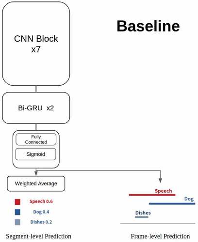
A baseline system is provided by Detection and Classification of Acoustic Scenes and Events (DCASE) Task 4 for sound event detection in domestic environments. The neural-network model in the baseline system consists of 7 convolution blocks and 2 bi-directional gated recurrent units (GRUs) and a prediction block. Each convolution block is composed of a 2D convolution layer, a batch normalization layer and a pooling layer. The kernel size of convolution layer in each convolution block is $3\times 3$ everywhere. All of the seven convolution blocks use gated linear units (GLU) as activation functions. The bi-directional GRUs have 128 cells. The prediction block is divided into two parts. One part is for frame-level prediction and the other part generates clip-level prediction from frame-level prediction. The frame-level prediction part is a simple fully connected layer with sigmoid activation function. The clip-level prediction part uses a linear layer and softmax layer to obtain an attention score and then it calculates attention-weighted sum of the frame-level prediction to generate clip-level prediction. Figure 1 shows the architecture of baseline system.

Figure 1. Baseline system: a CRNN model provided by DCASE task4 challenge. Each CNN block consists of a 3 × 3 convolution layer, a batch normalization layer, a GLU activation function, a dropout layer with 50% dropout rate and an average pooling layer. In the RNN part, there are two bidirectional GRU layers with 128 gated recurrent units. The CRNN model uses a fully connected layer and a sigmoid function to generate frame-level (strong) predictions, and then computes the clip-level (weak) predictions based on the frame-level predictions.

VGGSKCCT System

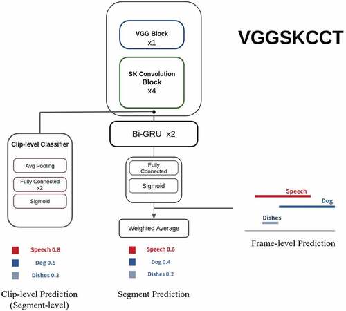
The implemented VGGSKCCT system is a blend of different models. It is based on the description of the system that won first place in 2021 DCASE Challenge Task 4 (Zheng, Chen, and Song 2021). It contains one VGG block, four residual blocks with selective kernel (SK), two bidirectional gated recurrent units and a prediction block. In VGGSKCCT system, we construct the blocks with our own settings. In addition and in contrast, we also add a new branch for clip-level consistency training (CCT). The name “VGGSKCCT” is derived from the VGG block, selective kernel and the clip level consistency training branch in this model. The system architecture is illustrated in Figure 2 and further implementation details are described below.

Figure 2. VGGSKCCT system: The CNN part combines one VGG block and four selective kernel units. Afterward, the system is composed of two branches. One branch is two bidirectional GRU layers and the prediction block, as in the baseline system, and the other branch is a CCT classifier.

VGG Block

The VGG block in this system is composed of two $3\times 3$ convolution layers, one batch normalization layer, one ReLU activation layer, one dropout layer with 0.5 dropout rate, and a $2\times 4$ average pooling layer.

Residual Blocks with Selective Kernel

The residual blocks in our system consist of two branches. The main branch consists of a $3\times 3$ convolution layer, a batch normalization layer, a selective kernel layer with $3\times 3$ and $5\times 5$ kernels, a dropout layer, another $3\times 3$ convolution layer, another batch normalization layer and an average pooling layer. The other branch is a residual/skip connection that connects the input feature map extracted by previous block to the output of the main branch. The output features of two branches are added and passed to a ReLU activation layer.

Bidirectional Gated Recurrent Units

In our system, the bi-directional gated recurrent units (GRUs) work in the same way as in the baseline system. This GRU-based recurrent neural network (RNN) is capable of extracting temporal features. There are 128 cells in an RNN layer with bi-directional GRUs.

Branch for Clip-Level Consistency Training

The branch for clip-level consistency training calculates the difference between clip-level outputs (which only predicts the occurrence of each event class). The idea is that the prediction of different networks should work well with a high-performance feature extractor. Furthermore, the clip-level prediction must remain the same regardless of whether more temporal features are extracted (by RNN) or not. This branch first downsamples the feature maps produced by the previous layer from {B, C, T, F} to {B, C $\times$ F, T}. Then, it uses an adaptive average pooling layer to combine the frame-level outputs. The shape of the feature maps is now {B, C $\times$ F}. Finally, the clip-level prediction is generated by two linear layers and a sigmoid layer. There is a loss associated with this branch to calculate the error between the main branch and CCT branch.

Prediction Block

In our system, the prediction block is exactly the same as that used in the baseline system. More details can be found in the previous section, which describes the baseline system.

Semi-Supervised Learning

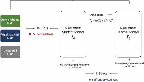
The mean teacher framework used in the baseline system is a semi-supervised method of learning. A typical mean teacher model is composed of two identical structures called the student model and the teacher model. As usual, the training data adjust the network parameters of the student model. In contrast, the parameters of the teacher model are calculated via the parameters of the student model using an exponential moving average. The following formula shows how a teacher model tunes its parameters

(1) ${\theta }_t^{\prime }=\alpha {\theta }_{t-1}^{\prime }+(1-\alpha ){\theta }_t$(1)

where $\theta$ and ${\theta }^{\prime }$ represent the parameters of the student model and teacher model, respectively, $t$ represents the current batch, and $\alpha$ is a hyper-parameter with a value between 0 and 1.

Loss Function

Loss Function of the Baseline System

The loss function contains two terms, namely the supervised loss (target loss) and the consistency loss

(2) $L_{\mathrm{t}\mathrm{o}\mathrm{t}\mathrm{a}\mathrm{l}}=L_{\mathrm{s}\mathrm{u}\mathrm{p}\mathrm{e}\mathrm{r}\mathrm{v}\mathrm{i}\mathrm{s}\mathrm{e}\mathrm{d}}+L_{\mathrm{c}\mathrm{o}\mathrm{n}\mathrm{s}\mathrm{i}\mathrm{s}\mathrm{t}\mathrm{e}\mathrm{n}\mathrm{c}\mathrm{y}}$(2)

The supervised loss is the binary cross entropy (BCE) between the predicted result generated by the student model ($\theta$) and the true answer on labeled data

(3) $L_{\mathrm{s}\mathrm{u}\mathrm{p}\mathrm{e}\mathrm{r}\mathrm{v}\mathrm{i}\mathrm{s}\mathrm{e}\mathrm{d}}=\mathrm{B}\mathrm{C}\mathrm{E}({\theta }_s(X_s),Y_s)+\mathrm{B}\mathrm{C}\mathrm{E}({\theta }_w(X_w),Y_w)$(3)

The consistency loss is the mean square error between the predictions of student and teacher models ($\theta { }^{\mathrm{\prime }}$) to quantify the discrepancy

(4) $L_{\mathrm{c}\mathrm{o}\mathrm{n}\mathrm{s}\mathrm{i}\mathrm{s}\mathrm{t}\mathrm{e}\mathrm{n}\mathrm{c}\mathrm{y}}=W\cdot \left\{\mathrm{M}\mathrm{S}\mathrm{E}[{\theta }_s(X),{\theta }_s^{\prime }(X)]+\mathrm{M}\mathrm{S}\mathrm{E}[{\theta }_w(X),{\theta }_w^{\prime }(X)]\right\}$(4)

Again, $\theta$ and ${\theta }^{\prime }$ represent the prediction of the teacher and student model, respectively. $X$ and $Y$ are the data and their corresponding labels. Subscripts $w$ and $s$ stand for clip-level and frame-level prediction, respectively.

Note the consistency loss is multiplied by an weight $W$ in Equation (4)(4) $L_{\mathrm{c}\mathrm{o}\mathrm{n}\mathrm{s}\mathrm{i}\mathrm{s}\mathrm{t}\mathrm{e}\mathrm{n}\mathrm{c}\mathrm{y}}=W\cdot \left\{\mathrm{M}\mathrm{S}\mathrm{E}[{\theta }_s(X),{\theta }_s^{\prime }(X)]+\mathrm{M}\mathrm{S}\mathrm{E}[{\theta }_w(X),{\theta }_w^{\prime }(X)]\right\}$(4) . Initially $W$ is set to a small number, so the model learns from the labeled data first and ignore the consistency between the student and teacher model. Specifically, the scheme of $W$ is

(5) $W=2\times e^{-5\ast \mathrm{p}\mathrm{h}\mathrm{a}\mathrm{s}{\mathrm{e}}^2}$(5)

where

(6) $\mathrm{p}\mathrm{h}\mathrm{a}\mathrm{s}\mathrm{e}=1-(\mathrm{c}\mathrm{u}\mathrm{r}\mathrm{r}\mathrm{e}\mathrm{n}\mathrm{t}\mathrm{s}\mathrm{t}\mathrm{e}\mathrm{p}/\mathrm{t}\mathrm{o}\mathrm{t}\mathrm{a}\mathrm{l}\mathrm{n}\mathrm{u}\mathrm{m}\mathrm{b}\mathrm{e}\mathrm{r}\mathrm{o}\mathrm{f}\mathrm{s}\mathrm{t}\mathrm{e}\mathrm{p}\mathrm{s}\mathrm{i}\mathrm{n}50\mathrm{e}\mathrm{p}\mathrm{o}\mathrm{c}\mathrm{h}\mathrm{s})$(6)

As the number of training steps increases, the weight also increases and the model begins to learn from the unlabeled data. The overall process is shown in Figure 3.

Figure 3. Mean teacher: a structure with two identical models. One is called “Student model” and the other is called “Teacher model.” In the training step, the prediction of the student model needs to be consistent with the ground truth labels and the prediction of the teacher model. After updating the parameters of the student model, the parameters of the teacher model are adjusted via the parameters of the student model using an exponential moving average.

Loss Function of the VGGSKCCT System

An additional term in the loss function is proposed to maintain the consistency of clip-level prediction on the two different branches in the VGGSKCCT system

(7) $L_{\mathrm{C}\mathrm{C}\mathrm{T}}=\mathrm{M}\mathrm{S}\mathrm{E}[{\theta }_w(X),{\theta }_{\mathrm{C}\mathrm{C}\mathrm{T}}(X)]+\mathrm{M}\mathrm{S}\mathrm{E}[{\theta }_w^{\prime }(X),{\theta }_{\mathrm{C}\mathrm{C}\mathrm{T}}^{\prime }(X)]$(7)

This term is a mean square error which computes the error of weak prediction generated by the two different branches. The first and second part in Equation 7(7) $L_{\mathrm{C}\mathrm{C}\mathrm{T}}=\mathrm{M}\mathrm{S}\mathrm{E}[{\theta }_w(X),{\theta }_{\mathrm{C}\mathrm{C}\mathrm{T}}(X)]+\mathrm{M}\mathrm{S}\mathrm{E}[{\theta }_w^{\prime }(X),{\theta }_{\mathrm{C}\mathrm{C}\mathrm{T}}^{\prime }(X)]$(7) means the clip-level consistency of the student and the teacher model, respectively, where ${\theta }_{CCT}$ and ${\theta }_{CCT}^{\prime }$ denote the predictions generated by the CCT branch of the student and teacher models. The other symbols are the same as in Equation 4.(4) $L_{\mathrm{c}\mathrm{o}\mathrm{n}\mathrm{s}\mathrm{i}\mathrm{s}\mathrm{t}\mathrm{e}\mathrm{n}\mathrm{c}\mathrm{y}}=W\cdot \left\{\mathrm{M}\mathrm{S}\mathrm{E}[{\theta }_s(X),{\theta }_s^{\prime }(X)]+\mathrm{M}\mathrm{S}\mathrm{E}[{\theta }_w(X),{\theta }_w^{\prime }(X)]\right\}$(4) This CCT loss is added to the consistency loss with the same weight used in the previous consistency loss. Thus, the consistency loss becomes

(8) $L_{\mathrm{c}\mathrm{o}\mathrm{n}\mathrm{s}\mathrm{i}\mathrm{s}\mathrm{t}\mathrm{e}\mathrm{n}\mathrm{c}\mathrm{y}}=W\cdot \left\{\mathrm{M}\mathrm{S}\mathrm{E}[{\theta }_s(X),{\theta }_s^{\prime }(X)]+\mathrm{M}\mathrm{S}\mathrm{E}[{\theta }_w(X),{\theta }_w^{\prime }(X)]+L_{\mathrm{C}\mathrm{C}\mathrm{T}}\right\}$(8)

Note the total loss still consists of supervised loss and consistency loss.

Loss Function of VGGSKCCT System with Knowledge Distillation

With knowledge distillation, the prediction of a pre-trained (often sophisticated) teacher model is used to guide a student (often simple) model. Normally, there is only one student and one teacher when using knowledge distillation. However, as we apply both knowledge distillation and mean teacher method in our system, our system has one student model and two teacher models. To distinguish the teacher models, we call the teacher model in knowledge distillation the “pre-trained teacher model.” The teacher model in mean teacher method is stilled called “mean teacher model.”

To distill knowledge from the pre-trained teacher model, we add another term to the consistency loss

(9) $L_{\mathrm{K}\mathrm{D}}=\mathrm{M}\mathrm{S}\mathrm{E}[{\theta }_w(X),{\theta }_w^{\mathrm{K}\mathrm{D}}(X)]+\mathrm{M}\mathrm{S}\mathrm{E}[{\theta }_s(X),{\theta }_s^{\mathrm{K}\mathrm{D}}(X)]$(9)

where the superscript $\mathrm{K}\mathrm{D}$ denotes the prediction of the pre-trained teacher model. $L_{\mathrm{K}\mathrm{D}}$ is similar to the loss between the mean teacher and the student model. It is based on mean square error, but it compares the student model with the pre-trained teacher model, instead of the mean teacher model. With the addition of knowledge distillation loss, the updated consistency loss is

(10) $L_{\mathrm{c}\mathrm{o}\mathrm{n}\mathrm{s}\mathrm{i}\mathrm{s}\mathrm{t}\mathrm{e}\mathrm{n}\mathrm{c}\mathrm{y}}=W\cdot \left\{\mathrm{M}\mathrm{S}\mathrm{E}[{\theta }_s(X),{\theta }_s^{\prime }(X)]+\mathrm{M}\mathrm{S}\mathrm{E}[{\theta }_w(X),{\theta }_w^{\prime }(X)]+L_{\mathrm{C}\mathrm{C}\mathrm{T}}+L_{\mathrm{K}\mathrm{D}}\right\}$(10)

Metric for System Performance

The polyphonic sound detection score (PSDS) (Bilen et al. 2019; Mesaros, Heittola, and Virtanen 2016) is an effective metric for sound event detection. PSDS counts the effective true positive rate under the effective false-positive rate. In the first step, it calculates the intersection between the prediction and the ground truth label from the aspect of each predicted event. It sets a hyper-parameter called detection tolerance criterion (DTC) to distinguish false positive samples by dividing the intersection by the length of prediction events and comparing if it is higher than DTC or not. In the second step, it does something similar. There is another hyper-parameter called ground truth intersection criterion (GTC). Unlike DTC, GTC is compared to the intersection divided by the length of each ground truth event. After passing through the threshold of DTC, it will then filter by GTC from another aspect of each ground truth event. Only the samples that pass through both DTC and GTC thresholds will be considered true positives (TPs). The third hyper-parameter in this metric is the cross-trigger tolerance criterion (CTTC). It counts how many samples are classified to the wrong class. Finally, the effective true positive rate is calculated by interpolating the mean and standard error of true positive ratios in each class with ${\alpha }_{ST}$. And the effective false-positive rate is calculated by interpolating false positive rate and cross trigger rate with ${\alpha }_{CT}$.

In 2021 DCASE Task 4, PSDS designed for different scenarios are adopted. PSDS1 sets hyper-parameters DTC to 0.7, GTC to 0.7, ${\alpha }_{ST}$ to 1, ${\alpha }_{CT}$ to 0 to emphasize accurate detection times of the sound event. PSDS2 sets hyper-parameters DTC to 0.1, GTC to 0.1, ${\alpha }_{ST}$ to 1, ${\alpha }_{CT}$ to 0.5, and CTTC to 0.3 to emphasize non-confusion between classes. We used the same metrics of PSDS1 and PSDS2 in this paper.

Data Augmentation

In order to further improve system performance, we use mixup (Hongyi et al. 2017) as a data augmentation technique. In the mixup method, two data samples are linearly combined to obtain a new data sample. That is

(11) $\hat{x}=\lambda x_i+(1-\lambda )x_j,\hat{y}=\lambda y_i+(1-\lambda )y_j$(11)

Here $x_i,x_j$ are the feature vectors of two randomly selected samples and $y_i,y_j$ represent the labels of these two samples. $\lambda$ is a parameter with a value between 0 and 1. $\hat{x}$ and $\hat{y}$ denote a newly generated sample and its corresponding label.

Post-Processing

The frame-level prediction is further post-processed to obtain the final output. We first convert each probability value into binary values with a threshold. The binary output is then passed through a median filter to further smooth the result and avoid spurious predictions. Our system uses the same post-processing setting as the baseline system. Specifically, all thresholds of event classes are 0.5 and the median filter size is 7 frames (i.e. about 0.45 s).

A Different Way to Use Knowledge Distillation

Knowledge distillation is frequently used to compress a model (Canwen et al. 2020; Sam and Rush 2020; Turc et al. 2019). It often exploits a pre-trained complex model with a better score to teach a simple model with a lower score. The two models are often referred to as the “teacher” and “student,” which is in line with the mean teacher framework. Similarly, there is a consistency loss to make the student model simulate the teacher model as well. In this way, we could transfer knowledge from teacher to student. The main difference between knowledge distillation and the mean teacher method is whether the teacher model will tune its parameters or not. Unlike the mean teacher method, the teacher model in knowledge distillation is pre-trained and will not tune its parameters in the training.

In this paper, we use knowledge distillation in a slightly different way. Specifically, the size of the pre-trained model to be learned from is not necessarily bigger than the model learning from the pre-trained model. Furthermore, we combine the mean teacher and knowledge distillation methods in training, so there are 2 teacher models and one student model in total. Our experiments show interesting results, that a simple teacher model in knowledge distillation can also benefit system performance. We deduce that the pre-trained model provided another type of prediction on weakly labeled and unlabeled data that increased model robustness. Also, we argue that the unusual results are due to the regularization effect stemming from limited data and model combination.

Apply Data Consistency Training to Knowledge Distillation with Two-Phase Training

Data consistency training is a common strategy in semi-supervised learning. The main idea is that the prediction of linear combination should be consistent with linear combination of the prediction. Applying this concept to the mean teacher architecture, the relationship between the student model and the teacher model can be strengthened. With input data $x_i$, we first generate the prediction $y_i$ with the teacher model in a mean teacher architecture. Then, we apply the same data augmentation (mixup) to both input data $x_i$ and the prediction $y_i$ to obtain $x_i^{\prime }$ and $y_i^{\prime }$, respectively. Following that, we produce the prediction $y^{\star }$ on $x_i^{\prime }$ based on the student model in the mean teacher architecture. Finally, we calculate binary cross-entropy between the labels $y_i^{\prime }$ and $y^{\star }$ to determine the loss of data consistency.

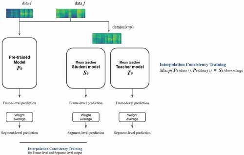
In our experiments, we use a special training scheme to incorporate consistency training in knowledge distillation and mean teacher method. We call it “two-phase training,” because the training process is split into two phases. In the first phase, we use the knowledge distillation as described above to develop a mean teacher model. In the next phase, we performed consistency training between the pre-trained model and the student model developed in the first phase. The prediction of the pre-trained model on the augmented sample should be in line with the prediction of the student model in the mean teacher architecture. Note this consistency training with the mixup method is also known as interpolating consistency training (ICT, Verma et al. 2019). In our consistency training scheme, the data of each batch have a 50% chance of being augmented using the mixup augmentation method. In addition, parameters of the pre-trained model will be updated during back-propagation, so the prediction of the pre-trained model could change slightly at each training epoch. With data consistency training, the student model could learn data diversity from the pre-trained model better, and improve its generalization ability. The training process is illustrated in Figure 4.

Figure 4. Second phase consistency training: the pre-trained model and (the student model in) the mean teacher model use consistency training with the mixup method. The input data in each batch has a 50% chance of being linearly combined. In addition, the parameters of the pre-trained model will be updated at the training step.

Results and Discussion

Experiment Setup

An input sound clip is converted to melspectrogram. We adjust the sampling rate of waveform to be identical (16 KHz) and pad all sound clips to the same length (12 s). In the conversion, we set the window size and hop length of short-time Fourier transform with 2,048 and 256 samples, respectively. The size of the fast Fourier transform is equal to 2,048 (same as the window size of STFT). The optimizer used in our experiment is Adam, and learning rate is updated by exponential warmup to reach maximum 0.001 after 50 epochs. Note that the scores shown in the tables are the higher value of the student or teacher model in the mean teacher framework.

The graphics processing unit (GPU) used in our experiment is GeForce GTX 1080 Ti 11 G. A training batch is composed of six clips with strong labels, six clips with weak labels and 12 clips without labels. The training process will last for 200 epochs without early stopping.

Comparison of Different Models

The first comparison is between the baseline system and the VGGSK system. From Tables 2 and 3, we can see the VGGSK system with a deeper and broader architecture outperforms the baseline system. A deep and broad architecture often performs well if it can overcome the vanishing gradient problem. Similar results are observed in the technical reports of DCASE2021 Task 4. Next, we compare VGGSKCCT system and VGGSK system to see the effect of clip-level consistency training. The second and third rows show the difference between using CCT or not. We can see that adding the CCT branch to the VGGSK system only improves PSDS2 on the validation set. This is because CCT loss only exploits weak predictions, and PSDS2 put more emphasis on the correct class labels than on the accurate times of occurrence (in contrast to PSDS1). Furthermore, the domain of validation set is similar to weak label data in training data set. Note the validation set is larger than the public evaluation set, so evaluation on the validation set is statistically more robust than on the public evaluation set. In subsequent system development, we keep the CCT branch in the system.

Table 2. Comparison of different models on the validation set: Comparison of different models on the validation set: The terms “Baseline,” “VGGSK” and “VGGSKCCT” denote the three systems in our experiment. Details can be found in Section Materials and methods.

	PSDS1	PSDS2
Baseline	0.341	0.546
VGGSK	0.409	0.618
VGGSKCCT	0.396	0.636

Table 3. Comparison of different models on the public evaluation set: Comparison of different models on the validation set: The terms “Baseline,” “VGGSK” and “VGGSKCCT” denote the three systems in our experiment. Details can be found in Section Materials and methods.

	PSDS1	PSDS2
Baseline	0.353	0.577
VGGSK	0.413	0.664
VGGSKCCT	0.405	0.656

Comparison of Different Training Methods

We next disclose the effect of using knowledge distillation and incorporating both the mean teacher method and knowledge distillation. The pre-trained model in knowledge distillation is similar to the aforementioned VGGSK system. The difference is it replaces the SK blocks with RepVGG (Reparameterized VGG) blocks (Ding et al. 2021) in order to decrease the number of model parameters from 2.5 m to 943k. This pre-trained model is also trained on the same DESED data. The first two rows in Tables 4 and 5 list the PSDS scores of VGGSKCCT system and pre-trained system with mean teacher framework. The third row is the knowledge distillation model with VGGSKCCT as a student model. This is referred to as 2-pass approach, since mean-teacher method and knowledge distillation method are applied in separate passes. The last row is a result of the model that includes a mean teacher model of VGGSKCCT and a pre-trained teacher model. This is referred to as 1-pass approach, since mean-teacher method and knowledge distillation method are applied simultaneously. The results in these tables indicate that when employing a pre-trained model to distill a VGGSKCCT model, there is no significant improvement. As we can see, the score of the student model and the pre-trained teacher model is roughly the same. The student model can only predict like a pre-trained teacher model if only knowledge distillation is used. However, the 1-pass approach, which incorporates both the mean teacher method and knowledge distillation, does improve performance. Here we also show the supervised losses of using 1-pass approach or not (mean teacher model with/without knowledge distillation) in Figure 5. The lighter line in the background is the true value of the supervised loss between strong labels and strong predictions. The darker line is the trend of the loss value. We can see that the pre-trained teacher model can assist the student model with the mean teacher structure in learning better, as the model that incorporates knowledge distillation and the mean teacher method decreases the loss more rapidly. Our argument for the improvement is that the 1-pass approach of incorporating knowledge distillation and the mean teacher method can be seen as model combination, which often improves system robustness especially with test set with high-performance variance.

Figure 5. Supervised loss: A figure with loss value and training step (number of total training batches). The blue one is a mean teacher model of VGGSKCCT trained in knowledge distillation (with a pre-trained model), and the red one is the same mean teacher model trained in a normal way. The lighter line in the background is the true value of the supervised loss between strong labels and strong predictions. The darker one in the foreground represents the trend in loss.

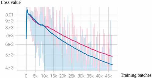
Table 4. Comparison of different training methods on the validation set: “Pre-trained” indicates a simple RepVGG model trained with the same data set. “VGGSKCCT_KD” indicates knowledge distillation with “Pre-trained” as a teacher model and the VGGSKCCT as a student model. “Vggskcct_kdmt” indicates incorporating knowledge distillation and the mean teacher method on the VGGSKCCT model.

	PSDS1	PSDS2
VGGSKCCT	0.396	0.636
Pre-trained	0.391	0.615
VGGSKCCT_KD	0.391	0.614
VGGSKCCT_KDmt	0.413	0.642

Table 5. Comparison of different training methods on the public evaluation set: “Pre-trained” indicates a simple RepVGG model trained with the same data set. “VGGSKCCT_KD” indicates knowledge distillation with “Pre-trained” as a teacher model and the VGGSKCCT as a student model. “Vggskcct_kdmt” indicates incorporating knowledge distillation and the mean teacher method on the VGGSKCCT model.

	PSDS1	PSDS2
VGGSKCCT	0.405	0.656
Pre-trained	0.420	0.655
VGGSKCCT_KD	0.420	0.655
VGGSKCCT_KDmt	0.437	0.667

Results of Combining One-Pass and Two-Stage Training Methods

This section presents the effect of two-phase training and data consistency methods on incorporating knowledge distillation and mean teacher models. In Tables 6 and 7, the first row lists results of VGGSKCCT in mean teacher trained with knowledge distillation, as is described in Subsection “Comparison of different training methods.” The second row lists the results of applying two-phase training to the model in the first row. The results show that updating the parameters of the pre-trained model with the second-phase training improves system performance. In particular, the PSDS2 gets a small increase on the validation set, and a significant improvement on the public evaluation set. The pre-trained model uses the loss between the student model and itself to adjust the parameters and improve the accuracy. This two-stage method can further increase the effect of knowledge distillation by providing labels with more accuracy. The third row in the tables lists the results of further using data consistency in the second phase of training. Compare to the second row, PSDS2 improves on both the validation set and the public evaluation set. From these results, we observe that the model can further benefit from data diversity with the mixup method.

Table 6. Comparison of two-phase training and data augmentation on the validation set: “Vggskcct_kdmt” is the same as that in Table 4 and 5. “Two-phase training” and “Two-phase training with ICT” indicate updating the parameters of the “Pre-trained” model and not only updating parameters but also using ICT, in the second phase, respectively.

	PSDS1	PSDS2
VGGSKCCT_KDmt	0.413	0.642
Two-phase training	0.410	0.647
Two-phase training with ICT	0.418	0.661

Table 7. Comparison of two-phase training and data augmentation on the public evaluation set: “Vggskcct_kdmt” is the same as that in Table 4 and 5. “Two-phase training” and “Two-phase training with ICT” indicate updating the parameters of the “Pre-trained” model and not only updating parameters but also using ICT, in the second phase, respectively.

	PSDS1	PSDS2
VGGSKCCT_KDmt	0.437	0.667
Two-phase training	0.436	0.683
Two-phase training with ICT	0.434	0.717

Conclusion

In this paper, we develop computation systems for sound event detection in domestic environments with deep-learning neural network models. Deepening or widening the convolution model and overcoming the gradient vanishing problem at the same time can strengthen the capability of a model. As shown by the results of our experiments, the proposed VGGSKCCT system, with deeper and broader capabilities than the baseline system, achieves better performance. Combining knowledge distillation and the mean teacher method to transfer knowledge from pre-trained model to student model, which can be seen as model combination, we observe further improvement in system performance. Finally, we apply a two-phase training procedure with interpolating consistency training in the second phase. Overall, these incremental changes to system design make the final system achieve better polyphonic sound detection scores for multiple sound event classes than state-of-the-art systems.

We will test the efficacy of the method by combining mean teacher and knowledge distillation on different datasets in future studies. It would also be worthwhile to test the method using the same model architecture (of mean teacher and pre-trained model) or using more pre-trained models to distill knowledge at the same time.

Acknowledgment

We would like to thank National Science and Technology Committee for funding this work. We would also like to thank the participating teams in the DCASE competition for sharing their methods to improve the performance by the technical reports.

Disclosure statement

No potential conflict of interest was reported by the author(s).

References

- Bilen, C., G. Ferroni, F. Tuveri, J. Azcarreta, and S. Krstulovic. 2019. A framework for the robust evaluation of sound event detection. arXiv preprint arXiv:1910 08440. https://arxiv.org/abs/1910.08440.
- Canwen, X., W. Zhou, G. Tao, F. Wei, and M. Zhou. 2020. BERT-of-Theseus: compressing bert by progressive module replacing. CoRr abs/2002.02925 https://arxiv.org/abs/2002.02925.
- Chih-Yuan, K., Y.S. Chen, Y.W. Liu, and M. R. Bai. 2021. Sound event detection by consistency training and pseudo-labeling with feature-pyramid convolutional recurrent neural networks. In ICASSP 2021 - 2021 IEEE International Conference on Acoustics, Speech and Signal Processing (ICASSP) Toronto, 376–19.
- Ding, X., X. Zhang, M. Ningning, J. Han, G. Ding, and J. Sun. 2021. RepVGG: making VGG-style ConvNets great again. CoRr abs/2101.03697 https://arxiv.org/abs/2101.03697.
- Endo, H., and H. Nishizaki. 2022. Peer collaborative learning for polyphonic sound event detection. In ICASSP 2022-2022 IEEE International Conference on Acoustics, Speech and Signal Processing (ICASSP) Singapore, 826–30. IEEE.
- Gulati, A., J. Qin, C.C. Chiu, N. Parmar, Y. Zhang, Y. Jiahui, W. Han, S. Wang, Z. Zhang, Y. Wu, et al. 2020. Conformer: Convolution-augmented transformer for speech recognition. arXiv preprint arXiv:2005 08100
- Hinton, G., O. Vinyals, and J. Dean. 2015. Distilling the knowledge in a neural network. In NIPS Deep Learning and Representation Learning Workshop, http://arxiv.org/abs/1503.02531.
- Hongyi, Z., M. Cissé, Y. N. Dauphin, and D. Lopez-Paz. 2017. Mixup: beyond empirical risk minimization. CoRr abs/1710.09412 http://arxiv.org/abs/1710.09412.
- Kaiming, H., X. Zhang, S. Ren, and J. Sun. 2015. Deep residual learning for image recognition. CoRr abs/1512.03385 http://arxiv.org/abs/1512.03385.
- Kim, N. K., and H. Kook Kim. 2021. Self-Training With Noisy Student Model And Semi-Supervised Loss Function For DCASE 2021 Challenge Task 4. Technical Report. DCASE2021 Challenge.
- Mesaros, A., T. Heittola, and T. Virtanen. 2016. Metrics for polyphonic sound event detection. Applied Sciences 6 (6):162. doi: 10.3390/app6060162.
- Miyazaki, K., T. Komatsu, T. Hayashi, S. Watanabe, T. Toda, and K. Takeda. 2020. Convolution-Augmented Transformer For Semi-Supervised Sound Event Detection. Technical Report. DCASE2020 Challenge.
- Nam, H., K. Byeong-Yun, G.T. Lee, S.H. Kim, W.H. Jung, S.M. Choi, and Y.H. Park. 2021. Heavily Augmented Sound Event Detection utilizing Weak Predictions. Technical Report. DCASE2021 Challenge.
- Park, D. S., W. Chan, Y. Zhang, C.C. Chiu, B. Zoph, E. D. Cubuk, and Q. V. Le2019SpecAugment: a simple data augmentation method for automatic speech recognitionInterspeech 2019sepISCA. http://doi.org/10.21437/2Finterspeech.2019-2680
- Sam, S., and A. M. Rush. 2020. Pre-trained summarization distillation. CoRr abs/2010.13002 https://arxiv.org/abs/2010.13002.
- Serizel, R., N. Turpault, A. Shah, and J. Salamon. 2020. Sound event detection in synthetic domestic environments. In ICASSP 2020 - 45th International Conference on Acoustics, Speech, and Signal Processing, Barcelona, Spain, May. https://hal.inria.fr/hal-02355573.
- Simonyan, K., and A. Zisserman. 2015. Very deep convolutional networks for large-scale image recognition. In International Conference on Learning Representations San Diego.
- Tarvainen, A., and H. Valpola. 2017. Weight-averaged consistency targets improve semi-supervised deep learning results. CoRr abs/1703.01780 http://arxiv.org/abs/1703.01780.
- Turc, I., M.W. Chang, K. Lee, and K. Toutanova. 2019. Well-read students learn better: on the importance of pre-training compact models. arXiv preprint arXiv:1908 08962.
- Turpault, N., R. Serizel, A. Parag Shah, and J. Salamon. 2019. Sound event detection in domestic environments with weakly labeled data and soundscape synthesis. In Workshop on Detection and Classification of Acoustic Scenes and Events, New York City, United States, October. https://hal.inria.fr/hal-02160855.
- Vaswani, A., N. Shazeer, N. Parmar, J. Uszkoreit, L. Jones, A. N. Gomez, Ł. Kaiser, and I. Polosukhin. 2017. Attention is all you need Advances in Neural Information Processing Systems Vancouver. 30.
- Verma, V., A. Lamb, J. Kannala, Y. Bengio, and D. Lopez-Paz. 2019. Interpolation consistency training for semi-supervised learning. In Proceedings of the 28th International Joint Conference on Artificial Intelligence, IJCAI Macao’19, 3635–41. AAAI Press.
- Xiang, L., W. Wang, H. Xiaolin, and J. Yang. 2019. Selective kernel networks. CoRr abs/1903.06586 http://arxiv.org/abs/1903.06586.
- Yang, L., J. Hao, Z. Hou, and W. Peng. 2020. Two-Stage domain adaptation for sound event detection. In Proceedings of the Detection and Classification of Acoustic Scenes and Events 2020 Workshop (DCASE2020), Tokyo, Japan, November, 230–34.
- Zheng, X., H. Chen, and Y. Song. 2021. Zheng USTC Team’s Submission For DCASE2021 Task4 – Semi-Supervised Sound Event Detection. Technical Report. DCASE2021 Challenge.