Advanced CNN Architectures for Pollen Classification: Design and Comprehensive Evaluation

ABSTRACT

Allergenic pollen affects the quality of life for over 30% of the European population. Since the treatment efficacy is highly related to the actual exposure to pollen, information about the type and number of airborne pollen grains in real-time is essential for reducing their impact. Therefore, the automation of pollen monitoring has become an important research topic. Our study is focused on the Rapid-E real-time bioaerosol detector. So far, vanilla convolutional neural networks (CNNs) are the only deep architectures evaluated for pollen classification on multi-modal Rapid-E data obtained by exposing collected pollen samples of known classes to the device in a controlled environment. This study contributes to the further development of pollen classification models on Rapid-E data by experimenting with more advanced concepts of CNNs, residual, and inception networks. Our experiments included a comprehensive comparison of different CNN architectures, and obtained results provided valuable insights into which convolutional blocks improve pollen classification. We propose a new model which, coupled with a specific training strategy, improves the current state-of-the-art by reducing its relative error rate by 9%.

Introduction

Pollen grains are structures in seed plants that protect male genetic material during transfer to female reproductive organs in sexual reproduction. About 25% of vascular plants utilize wind for pollination (Culley et al. 2002). To increase success in fertilization, they rely on producing large quantities of pollen, exposed male flowers and anthers to simplify emission and improve the efficiency of aerodynamic properties of pollen grains to facilitate atmospheric dispersion. Anemophilous pollen grains are small, often circular with smooth surfaces and sometimes bearing additional structures that decrease their specific weight (i.e., air compartments or sacks).

During the flowering period, exposure to airborne pollen grains from wind-pollinated plants triggers allergic reactions and significantly decreases the quality of life for 30% of the world population sensitive to pollen (Burbach et al. 2009). The sensations related to pollen are getting increasingly intense over time and can induce severe effects on health (Beggs 2017). The timing of flowering and pollen emission is species-specific and driven by environmental factors such as temperature and photoperiod (Dahl et al. 2013). Furthermore, the production and emission of pollen depend also on factors related to human activity, i.e., land use change and introduction of new species leading to the occurrence of new pollen types and global warming and increase of atmospheric CO2 leading to changes in timing and intensity of pollen season (Dahl et al. 2013).

Since the treatment efficacy for allergic diseases is highly related to exposure to pollen (de Weger et al. 2021), the information on the type and number of pollen allergens suspended in the air is essential for preventing their symptoms. Besides timely information on exposure levels, pollen concentrations can be used to figure out trends in the annual rhythms of plants and anthropogenic changes (Ziska et al. 2011), in forestry research (Kasprzyk, Ortyl, and Dulska-Jez 2014) or crop forecasts (Oteros et al. 2014). Coupled with meteorological data, changes in the timing and intensity of pollen season can be monitored, which can be relevant to monitoring climate change (D’Amato et al. 2007). Finally, real-time measurements are of particular importance quality of forecast products since, as in meteorology, the assimilation of observation data is expected to improve the accuracy of predictions notably (Sofiev 2019).

Pollen identification is still done mostly manually with volumetric Hirst-type traps (Hirst 1952), where pollen impacts a moving adhesive tape, and the samples are examined manually with a microscope (Buters et al. 2018). Pollen can be easily discriminated against other bioaerosols using microscopic images. Methodology with Hirst allows pollen identification typically at the genus or family level, although within some groups, it is even possible at the species level (Bennett and Willis 2002). However, this manual method of counting pollen has apparent problems. Not only is it time-consuming and labor-intensive, but the information about pollen quantity is also delayed from a few days up to a few weeks. Furthermore, manual measurements have an error rate, which depends on the sampled area and the number of particles suspended in the air (Buters et al. 2022; Matavulj et al. 2022). Additionally, they are subjected to human errors and mistakes. However, several factors can also affect the accuracy of automatic measurements (Buters et al. 2022). But the biggest problem of manual measurements, which became apparent with the introduction of new pollen monitoring networks, is the lack of scalability since it requires additional time and a specialized workforce. Despite all the issues, this method still represents the standard for pollen monitoring. Up to 2018, only 8 out of 525 pollen samples were automatic in Europe (Buters et al. 2018).

However, recent years have witnessed fast development of devices applying a wide range of methods capable of bioaerosol detection in real-time (Huffman et al. 2019; Tummon et al. 2021). The device employed for this research is the Rapid-E real-time bioaerosol detector (Plair SA), which collects scattered light patterns and fluorescence information in real-time, representing particles’ morphological and chemical characteristics (Sauliene et al. 2019). Even though scattered light images explain the morphological characteristics of particles, the distinction of different pollen is not comparable to the discrimination using microscopic images since the device works on another principle. Furthermore, the dataset containing particles recorded by Rapid-E and labeled for 24 pollen classes and two classes representing other (bio)aerosols were available for training the classification models (Tesendic et al. 2020).

Our work further contributes to the development of pollen classification models by adjusting more advanced concepts of CNNs, residual and inception networks, on Rapid-E data since they yielded better results on other datasets than vanilla CNNs (Krizhevsky, Sutskever, and Hinton 2012; Simonyan and Zisserman 2015). The motivation for this work is to improve on the current state-of-the-art results by proposing a high-performance solution to the problem of pollen classification. Since the models classify 1-minute files in milliseconds, the classification time in real-time is not critical. Therefore, our research focused on comprehensive experimental comparisons of different CNN architectures, which provided valuable insights into which computational FE blocks can extract more discriminatory information and improve pollen classification on Rapid-E data when coupled with a specific training strategy.

Related Work

Since pollen classification has been heavily relying on grains’ morphological characteristics, many techniques based on microscopy have been developed, where deep learning models generally performed better than classic machine learning models (Viertel and König 2022). However, most techniques are not feasible in real time except for digital microscopy, where images are captured and analyzed automatically (Buters et al. 2022). This technique is implemented in the Helmut Hund BAA500, PollenSense APC, ACPD, and Aerotrap devices, where only for BAA500 device published peer-reviewed publications can be found. The algorithm segments particles of interest and classifies them (Oteros et al. 2020; Plaza et al. 2022). For segmentation and classification, deep learning methods yielded better results than classic machine learning algorithms (Boldeanu et al. 2022; Schiele et al. 2019). Besides digital microscopy, several other techniques for automatic pollen detection exist based on light-induced methods. Those include spectroscopy, scattering, and holography, where signals from single particles exposed to laser light are used for describing pollen morphological and chemical characteristics (Buters et al. 2022). Those techniques are applied in the Rapid-E (Plair), Poleno (Swisens), WIBS (Droplet Measurement Technologies), and KH-3000 (Yamatronics) devices. Sauvageat et al. (2020) have recognized six out of eight pollen taxa with an accuracy above 90%, combining the Polenos’ holography method with deep learning. However, the extension to other pollen taxa remains to be tested. O’Connor et al. (2014) obtained a strong positive correlation >0.9 for total pollen compared with Hirst data by implementing a fluorescence intensity threshold on the WIBS device. But no individual pollen taxa have been classified. Furthermore, with the KH-3000 device, Kawashima et al. (2007) obtained a positive correlation (>0.7) when compared with Hirst data for only three out of six pollen taxa since the device is designed to quantify particles in a predefined size range.

Recent studies addressing pollen classification on Rapid-E data experimented with CNN-based type of models, primarily because of the Rapid-E data heterogeneity but also because of its noisiness which can be successfully suppressed with CNNs (Boldeanu et al. 2021; Matavulj et al. 2021; Sauliene et al. 2019; Tesendic et al. Simonyan and Zisserman 2015). CNNs operate automatic feature extraction. They are more noise resistant and perform better than classical machine learning algorithms on other datasets (Sothe et al. 2020). So far, vanilla CNNs are the only CNN types experimented for pollen classification on Rapid-E data (Boldeanu et al. 2021; Sauliene et al. 2019; Simonyan and Zisserman 2015). Sauliene et al. (2019) tested multiple networks consisting of different numbers of layers, number of feature maps in convolutions, kernel sizes in convolutional layers, number of network nodes, and adding regularization layers like dropout, batch normalization, and maxpool with different parameters. The architectures of the best FEs for each input are given in Table 1. Obtained features are then equalized in length by one fully-connected layer, concatenated, and the classification is performed (Figure 1).

Figure 1. Multi-modal neural network architecture.

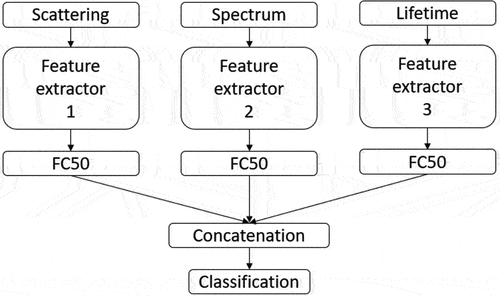
Table 1. Feature extractors for each data type. Numbers in the convolution brackets correspond to the number of feature maps and the kernel size, respectively.

Scattered light image	Fluorescence lifetime	Fluorescence spectrum
batch normalization convolution(10, 5) relu activation	batch normalization convolution(70, (1, 7)) relu activation	batch normalization convolution(50, (1, 5)) relu activation
batch normalization convolution(20, 3) dropout(0.5) relu activation	batch normalization convolution(140, (1, 5)) relu activation	batch normalization convolution(100, 3) dropout(0.5) relu activation
	batch normalization convolution(200, 3) dropout(0.5) relu activation

A multi-modal convolutional neural network (CNN) has been trained to identify 24 pollen taxa with 65% accuracy (Simonyan and Zisserman 2015). This classification model was implemented in a system for automatic pollen classification and tested against the standard sampling with a Hirst-type method, obtaining a strong positive relationship with more than 0.5 Spearman’s correlation coefficient for 14 out of 22 pollen classes (Simonyan and Zisserman 2015), and further research showed they could also detect starch particles in the ambient air with the same model (Sikoparija et al. 2022). Boldeanu et al. (2021) improved the results by firstly training a CNN for each mode separately and then using the pretrained weights in a multi-modal network, which is why we implemented that training strategy. They reduced the error rate by 13% (Boldeanu et al. 2021), which is the current state-of-the-art in terms of accuracy. However, they used a reduced number of pollen classes.

To find the best model for pollen classification with Rapid-E data, we modified and tested more advanced concepts of FEs that performed better on the ImageNet dataset (Krizhevsky, Sutskever, and Hinton 2012; Simonyan and Zisserman 2015). These include residual networks (He et al. 2016), inception networks (Szegedy et al. 2015) and their improvements, Wide ResNet (Zagoruyko and Komodakis 2016), and ResNeXt (Xie et al. 2017). We have also tested the most famous vanilla CNNs: AlexNet (Krizhevsky, Sutskever, and Hinton 2012) and VGG net (Simonyan and Zisserman 2015), but only on the scattered light image since these models require bigger spatial dimensions of the input data. We compared those models with the state-of-the-art on Rapid-E data, which includes models with hyperparameters implemented from previous research (Sauliene et al. 2019; Simonyan and Zisserman 2015) coupled with a training strategy for multi-modal networks that involves training each mode separately and then combining them in one network (Boldeanu et al. 2021).

Models

Vanilla CNNs

FEs in Vanilla CNNs have a basic structure comprising layers stacked on each other. The input goes through one layer at a time in the order in which they are stacked. One of the most famous vanilla CNN is the AlexNet, the first end-to-end deep learning model that won the ImageNet challenge in 2012 (Krizhevsky, Sutskever, and Hinton 2012). Simonyan and Zisserman, 2015 replaced the 11 × 11 and 5 × 5 filters of AlexNet with a stack of 3 × 3 filters in the VGG network to reduce the number of parameters. However, the increased number of layers in the VGG network made the problem of vanishing gradient more apparent. While VGG networks are simple, they are still very computationally expensive (Simonyan and Zisserman 2015).

We implemented the AlexNet and the VGG16 network. Since these networks have big receptive fields, it was impossible to implement them on fluorescence data. Therefore, we implemented VGG16 and AlexNet only on scattered light images. In AlexNet, we changed the first convolutional layer to have a 5 × 5 kernel size and no stride. Furthermore, we changed the final layer in both networks since our number of classes differs from the original network.

Residual Networks

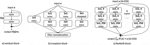
As convolutional networks get deeper, the accuracy starts to saturate (He et al. 2016). ResNet is considered a solution for degrading accuracy in deeper networks. He et al. (2016) introduced shortcut connections that allow information to pass without any transformation, which is data-independent and parameter-free, so there are no additional computational costs. Those connections can be considered as obtaining a slightly altered representation of the input: as it passes through convolutional layers, the input x is transformed by some function F to F(x), representing edges, shapes, etc. of the original image. Therefore, x + F(x) represents a slight change in the input image (Figure 2a). The authors suggested that the residual functions can gain accuracy with increased network depth. The shortcut connections enabled the convergence speedup for deep networks. Furthermore, they solved the vanishing gradient problem since the gradients can flow directly through the skip connections backward from later layers to the first layer without losing information (He et al. 2016).

Figure 2. Convolutional blocks of different CNN type.

We implemented an 18-layer residual network (ResNet18), where the reduction in spatial dimensions is achieved by increasing the stride instead of pooling operations (He et al. 2016). For the lifetime and spectrum data, the first convolutional layer was modified to take as input a monochrome image and implement a kernel of size 5 × 5, padding of 2 × 2, and no stride to save the dimensions. The final fully-connected layer was replaced for all three inputs to fit our classification problem regarding the number of classes. Even though ResNet18 is the smallest of the bunch, we wanted to experiment with even smaller networks to fit our dataset of small spatial dimension images. For that reason, we implemented ResNets that have from one to five residual blocks, with the Global Average Pooling (GAP) and without it. The networks with four and five residual blocks were prone to overfitting, so we introduced dropout to these networks to obtain better results.

Inception Network

To reduce the computational costs of CNNs while achieving state-of-the-art accuracy, Szegedy et al. (2015) proposed the inception block in GoogleNet, which was an important milestone for CNN development. Instead of going deeper by stacking convolutional layers on top of each other, the inception network implements wide inception blocks, which summarize filters of different sizes to obtain spatial information at various scales (Figure 2b). Input in the inception module convolves with three different filter sizes (1×1, 3 × 3, 5 × 5) and one max pooling layer. To make the network computationally cheaper, a bottleneck convolutional layer with a 1 × 1 filter is introduced before other large-size filters, except for the max pooling layer. The resulting outputs are concatenated and sent to the next module. In this way, the number of input channels is limited, and even though we are doing extra operations, the reduced number of input channels makes it worth it (Szegedy et al. 2016). Furthermore, GoogleNet introduced the concept of auxiliary learners to speed up the convergence rate by dealing with the vanishing gradient problem, which prevents the middle part of the network from “dying out” (He et al. 2016; Szegedy et al. 2015). In addition, GAP was used at the last layer instead of a fully connected layer, further decreasing the parameters from 138 million to 4 million (Szegedy et al. 2015).

Similarly, as with ResNets, the first convolutional layer in GoogleNet for lifetime and spectrum data was replaced with the one with a kernel size of 5 × 5, a stride of 1 × 2, and padding of 2 × 2. The auxiliary and the final fully connected layers were replaced for all three inputs to output a vector of size 26, the number of classes for our specific problem. We also implemented GoogleNet with one to four inception blocks.

Wide Residual Networks

In deep residual networks, there is a possibility that some residual blocks do not learn anything since there is nothing to force the gradients to go through them. Therefore, they may contribute very little or nothing to learning, so a dropout was added between the convolutional layers instead of within a residual block, which forces the network to use all residual blocks (Srivastava, Greff, and Schmidhuber 2015). This idea was implemented by Zagoruyko and Komodakis (2016) in the Wide Residual Networks. They thought that the potential of ResNets lies in their residual units and therefore wanted to exploit the residual blocks to make a network wider than deep by increasing the number of feature maps in the convolutional layers.

We have implemented 50 layers deep Wide ResNet with a widening factor of 2. Note that the Wide ResNet with a widening factor of 1 is just ResNet. For fluorescence spectrum and lifetime data, the first convolutional and pooling layers were adapted to convolve and stride just over the image’s width since the height of these images is only 4 pixels. The final fully connected layer is adapted for all inputs to fit this classification problem.

ResNext

Xie et al. (2017) introduced the term “cardinality” to improve the inception network, which refers to the size of the inception block. They showed that an increase in cardinality significantly improves performance (Szegedy et al. 2015). ResNeXt simplified GoogleNet by fixing the receptive field of the convolutional layers to 3 × 3 filters while still using residual learning to improve the convergence (He et al. 2016; Szegedy et al. 2015). The complexity of ResNeXt was regulated by applying 1 × 1 filters before 3 × 3 convolution (Larsson, Maire, and Shakhnarovich 2016).

We implemented 50 layers deep ResNeXt with the cardinality of N = 32 and the dimension of d = 256 (Figure 2c). ResNet 50 is a special case of ResNeXt 50 with a cardinality of 1 and a dimension of 64. Similarly, as for the Wide ResNets, the first convolutional and pooling layers were adapted to convolve and stride just over the image’s width for fluorescence spectrum and lifetime data. The final fully connected layer is adapted to output 26 classes for all inputs.

Dataset

Technology and Data

Laser-induced bioaerosol detector Rapid-E, produced by Plair SA, is an automated instrument that continuously samples surrounding air and records airborne particles in real-time. It works on two physical principles by interacting with the particles with a deep-UV and an infra-red laser, resulting in scattered light and fluorescence patterns representing information about their morphological and chemical properties (Sauliene et al. 2019). It can detect particles of size 0.5–100 µm. However, the device employed for these experiments worked in the “smart pollen” mode, where only particles with an approximated size greater than 8 µm in optical diameter were detected (Sikoparija et al. 2019).

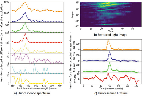
The first interaction of an infra-red laser with a particle is collected by 24 spectral detectors representing different angles in the range of 45 to 135 degrees relative to the laser light beam. Particles are illuminated multiple times depending on their size and shape, and the scattered light image is obtained, where the image’s width is not fixed. Additionally, a deep-UV laser excites the particle at 337 nm as it passes down the chamber. Light is collected by the 32 spectral detectors representing the particles’ emission wavelength in the range of 350 to 800 nm. The collection of light is repeated eight times with an interval of 500 ns. The laser light is then rotated to a second direction and interacts with a particle once again when the fluorescence duration is measured for four spectral ranges: 350–400 nm, 420–460 nm, 511–572 nm, and 672–800 nm (Figure 3).

Figure 3. Data instance of class Betula.

Labeled Dataset

The labeled dataset for classification was available from the previous research study on pollen classification (Simonyan and Zisserman 2015). It is obtained by exposing the device to collected pollen samples in controlled environmental conditions. This process takes a few minutes for each class, provided that the pollen samples are already collected beforehand (Sauliene et al. 2019). The 24 pollen classes (not referred to the taxonomical rank) are represented in training set by pollen from one or more plant taxa as described in Matavulj et al. (2022), e.g., the class Artemisia consists of pollen from Artemisia absinthium L. and Artemisia vulgaris L. The dataset includes the following classes: Acer (ACER), Alnus (ALNU), Ambrosia (AMBR), Artemisia (ARTE), Betula (BETU), Broussonetia (BROU), Carpinus (CARP), Corylus (CORY), Fraxinus excelsior (FRAX E), Fraxinus ornus (FRAX O), Juglans (JUGL), Morus (MORU), Pinaceae (PINA), Plantago (PLAN), Platanus (PLAT), Poaceae (POAC), Populus (POPU), Quercus (QUER), Salix (SALI), Taxaceae (TAXA), Tilia (TILI), Ulmus (ULMU), Urticaceae (URTI) and one class representing a collection of other pollen taxa which are present in air but in very low quantity (OTHER P). This class resulted in a low classification score in a previous study (Simonyan and Zisserman 2015). The results showed that the class is not contributing to the classification. However, we decided to keep it for the comparison of the results. Furthermore, we collected air measurements when no pollen was present in the ambient air, which included spores, starch, and other fluorescent material, represented by two additional classes in the dataset (STARCH, SPORES), so in the operational settings, the labeled dataset can better represent the variability of airborne particles.

Data Filtering and Preprocessing

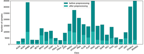
The collected labeled dataset contains three types of measurements gathered for 535 718 particles. However, some particles have low-quality signals, which are filtered out from the dataset. Measurements with a scattered light image width lower than 450 pixels, a maximum lifetime index between 10 and 44, a maximum spectrum intensity higher than 2500, and four maximum spectrum indices between 3 and 10 are kept for further analysis. After filtering, measurements for 104 825 particles are included in the labeled dataset, representing 20% of all measured particles. The number of data samples per class is given in Figure 4. Furthermore, data is preprocessed by centering the scattered light image, fixing its width, and removing two pixels from the top and bottom due to device dependence. Finally, the fluorescence signals are converted into images as in Simonyan and Zisserman (2015) and normalized into the 0–1 range. Moreover, the signals of scattered light and fluorescence spectrum are smoothed. Detailed preprocessing steps are explained in Simonyan and Zisserman (2015).

Figure 4. Number of data samples per class (abbreviations defined in the Labeled dataset subsection) before and after preprocessing. The y-axis is limited for visibility since classes Poaceae and spores have 82,143 and 157,753 samples before preprocessing, respectively.

Experiments and Results

Experimental Setup

We split the labeled dataset into train, validation, and test datasets. The training dataset used for training the models contains 80% of the data for each class, and the rest is split into validation and test datasets, containing 10% of data each. The former is used to tune the hyperparameters of models and validate their performance during training, and the latter to test the best-performing model to ensure there is no overfitting on the validation set. The impossibility of counting collected pollen grains before bulk sample for each pollen class passes through the device and the different percentages of discarded samples with preprocessing due to pollen particles’ morphological and chemical properties resulted in an imbalanced dataset. Therefore we created batches by sampling procedure that represents all classes equally. The batch size was 260, containing ten samples per class. Each batch takes ten new samples of each class until there are no new ones. Then, the samples start repeating in the same order. The sampling procedure for creating batches is done only once; therefore, all models were trained with the same order of data. The only difference was the training time – models with the lowest validation error were saved. Therefore, some models were trained with more epochs than others. All models implemented the log-softmax activation function and calculated loss with the negative log-likelihood function. The optimization is performed with the stochastic gradient descent with 0.9 momentum, and the learning rate was 0.0001 for uni-modal models and 0.001 for multi-modal networks. For faster training of the models, GPU acceleration was used. Since we have an imbalanced dataset, we have chosen to evaluate our models using accuracy, precision and recall, and F1 score. The precision measures how good the model is at classifying a sample as the correct class, the recall measures how correct are the predictions for one class, and the F1 score is defined as the harmonic mean of the precision and recall. Because we have a multiclass problem, the precision, recall, and F1 score are calculated for each class, weighted by the number of samples of that class, and then averaged, which can result in an F1 score that is not between precision and recall.

Uni-Modal Networks

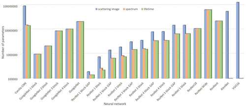
For each of the inputs independently, we trained different networks: ResNet, GoogleNet, ResNet Wide, and ResNeXt, while for scattering images, we trained two more: AlexNet and VGG. All networks were trained with weights initialized randomly and weights trained on the reduced ImageNet dataset (Krizhevsky, Sutskever, and Hinton 2012; Simonyan and Zisserman 2015) Along with these networks, we have trained vanilla CNNs, adjusted GoogleNet with one to four inception blocks, and adjusted ResNet that has one to five residual blocks, with and without GAP (Hsiao et al. 2019). Since the four and five-block networks were prone to overfitting, we introduced dropout to those networks. Figure 5 shows the number of trainable parameters for each described network and input. Some networks have the same number of parameters no matter the input: GoogleNets, ResNet18, Wide ResNet, and ResNeXt, while the variations of ResNets with GAP have the same number of parameters for the fluorescence spectrum and lifetime.

Figure 5. Number of parameters for each network and data type in a logarithmic scale.

Table 2 shows the results obtained with different networks for the scattered light image, fluorescence spectrum, and fluorescence lifetime data. Among the top-5 worst performing networks for each data type were Wide ResNet and ResNeXt, with random weights and weights pretrained on the ImageNet dataset. These networks were prone to overfitting after a few epochs, probably since the data was too small and contained a lot of noise. Furthermore, the variations of GoogleNet also had a low performance for the scattered light image, implying that the width of the inception module is not suitable for this data type and that sufficiently discriminatory features can be obtained without the width of the convolutional block. This is further noticeable for the fluorescence lifetime data, where the difference between the best GoogleNet and the best ResNet was around 10%.

Table 2. Performances of the uni-modal networks.

	Accuracy	Precision	Recall	F1 score
Scattered light image
Vanilla CNN	0.438	0.434	0.438	0.436
Best GoogleNet	0.427	0.445	0.427	0.436
Best ResNet	0.478	0.507	0.478	0.493
Wide ResNet	0.394	0.392	0.394	0.393
ResNeXt	0.400	0.414	0.400	0.407
AlexNet	0.460	0.492	0.460	0.476
VGG16	0.432	0.448	0.432	0.440
Fluorescence spectrum
Vanilla CNN	0.434	0.475	0.434	0.454
Best GoogleNet	0.447	0.459	0.447	0.453
Best ResNet	0.461	0.490	0.461	0.475
Wide ResNet	0.411	0.421	0.411	0.416
ResNeXt	0.399	0.438	0.399	0.419
Fluorescence lifetime
Vanilla CNN	0.493	0.489	0.493	0.490
Best GoogleNet	0.398	0.420	0.398	0.409
Best ResNet	0.492	0.510	0.492	0.501
Wide ResNet	0.319	0.320	0.319	0.319
ResNeXt	0.332	0.334	0.332	0.333

The top-5 best-performing networks were variations of ResNet, no matter the data type. The networks that implemented GAP performed the best for scattered light images, while for the fluorescence spectrum data, these were without GAP. This implies that for scattered light images, enough information can be preserved just by averaging the data over the spatial dimensions and that there is no need for fully-connected layers, which can introduce much more complexity to the models (Figure 5), while for the fluorescence spectrum data, there is more information than what is preserved after averaging and this information is best exploited with the fully-connected networks. In other words, the number of feature maps is not enough for the spectrum data to be expressed in a way to contain the most information. For the fluorescence lifetime data, four of the top-5 best-performing networks included four and five-block ResNets, with and without GAP. The difference between them varies around 4%, but the clear winners are four-block ResNet and a vanilla CNN, and it’s a tossup between them (Table 2). For scattered light images, the best performance was obtained with a three residual block-ResNet using GAP, outperforming the vanilla CNN by 5% in accuracy and F1 score, while for the fluorescence spectrum also a three residual block-ResNet performed the best, this time without GAP, improving the vanilla CNN results by approximately 2.5%. The difference between the worst and the best performing networks overall was the biggest for the fluorescence lifetime data as it is around 20%. The results are the most stable for the fluorescence spectrum data, for which the difference was around 7%. For the scattered light image, the difference was 13%.

Multi-Modal Networks

After training the networks for each of the inputs separately, the FEs of the best performing models, which were different variations of ResNets, were implemented in a multi-modal network, along with the vanilla CNNs for comparison with previous studies (Sauliene et al. 2019; Simonyan and Zisserman 2015). We can have multiple training strategies when dealing with multi-modal networks (Boldeanu et al. 2021):

1. Train the model with random initialization of FE weights – weights not yet learned from the data. However, this approach disables the use of different learning rates or training times for different FEs, which can be a problem since some FEs can train faster than others, depending on the architecture of the FE, leading to some FEs overfitting while others are not fully trained yet (Boldeanu et al. 2021)

2. Train the model with random initialization of FE weights and with intermediate outputs, as in (Boldeanu et al. 2021) - not only does the network classify with the common fully-connected layers, but each input does its separate classification, which should exploit FE layers for each of the inputs to the best of their abilities (Boldeanu et al. 2021). Here, the loss can be calculated in different ways. We have explored two options, one as recommended in (Boldeanu et al. 2021), and a straightforward summation of the losses:

   (1) $\mathrm{L}={\mathrm{L}}_{\mathrm{m}\mathrm{a}\mathrm{i}\mathrm{n}}+0.1\ast \left({\mathrm{L}}_{\mathrm{s}\mathrm{c}\mathrm{a}\mathrm{t}\mathrm{t}\mathrm{e}\mathrm{r}\mathrm{i}\mathrm{n}\mathrm{g}}+{\mathrm{L}}_{\mathrm{s}\mathrm{p}\mathrm{e}\mathrm{c}\mathrm{t}\mathrm{r}\mathrm{u}\mathrm{m}}+{\mathrm{L}}_{\mathrm{l}\mathrm{i}\mathrm{f}\mathrm{e}\mathrm{t}\mathrm{i}\mathrm{m}\mathrm{e}}\right)$(1)
   (2) $\mathrm{L}={\mathrm{L}}_{\mathrm{m}\mathrm{a}\mathrm{i}\mathrm{n}}\hspace{0.17em}+{\mathrm{L}}_{\mathrm{s}\mathrm{c}\mathrm{a}\mathrm{t}\mathrm{t}\mathrm{e}\mathrm{r}\mathrm{i}\mathrm{n}\mathrm{g}}+{\mathrm{L}}_{\mathrm{s}\mathrm{p}\mathrm{e}\mathrm{c}\mathrm{t}\mathrm{r}\mathrm{u}\mathrm{m}}+{\mathrm{L}}_{\mathrm{l}\mathrm{i}\mathrm{f}\mathrm{e}\mathrm{t}\mathrm{i}\mathrm{m}\mathrm{e}}$(2)

3. Train the whole model (FEs and the classifier) with pretrained FE weights – FE weights are first learned on each input separately and then utilized in the multi-modal network. If we train each FE independently, we can choose different learning rates and training times for each FE. That way, we can obtain an optimal solution for each data type (Boldeanu et al. 2021). However, training the whole multi-modal network with a classifier that is not yet learned can corrupt the FE weights previously learned on each input separately. Therefore, we utilized the following strategy:

4. Training just the model’s classifier with pretrained FE weights – training just the fully-connected part of the network, the FE weights are frozen during training, i.e., they are not changed

5. unfreezing the FE layers of the model learned with the training strategy 4. and fine-tuning it

Figure 6 shows the results of training multi-modal vanilla CNNs and ResNets by applying the previously described training strategies. As noticed in some other studies (Boldeanu et al. 2021; Sauliene et al. 2019), the results of the multi-modal classification exceed the performance of any uni-modal network trained on an individual feature, making the features seem complementary. With each learning strategy, we observed an increase in the performances of both models. Multi-modal vanilla CNN outperforms ResNet when FE weights are initialized randomly in both training settings: training with just one classifier (by 4%) or with intermediate classifiers with loss defined as (2) (by 1%). Training a network with intermediate outputs with the loss is defined as (1) yielded worse performance for both vanilla CNN and ResNet, where the difference for vanilla CNN was 2%, while for ResNet, it was 12%. The performances of both models are equal when the whole network is trained with pretrained FE weights. The results when the pretrained FE weights are frozen are better for both models, which makes sense since training a whole network with random weights for the classifier yields too big of a step in which the weights are updated at the beginning of the training.

Figure 6. F1 score of multi-modal networks for different training setups.

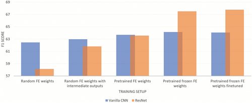
The direct comparison of model performances with the state-of-the-art on Rapid-E data is impossible since the authors of that work used a different dataset containing only 11 classes (Boldeanu et al. 2021). However, by implementing a training strategy (4), we obtained a model on our dataset comparable with the state-of-the-art: a multi-modal vanilla CNN with pretrained features. As a result, the ResNet network now outperforms vanilla CNN by 4%, obtaining a relative reduction in the error rate of 9%. Fine-tuning the networks improves the classification performance, although very little. It should be noted that a multi-modal ResNet has 13.9 million parameters, 5.6 times more than a multi-modal vanilla CNN.

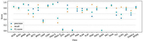
Analyzing the confusion matrix of the best classification model (Figure 7), we observe that most classes have good classification: four classes have a > 90% classification rate, nine have between 80% and 90%, and five have between 70% and 80%. The confusion between Alnus, Betula, Corylus, and Quercus is expected since they have similar morphology and fluorescence patterns (Boldeanu et al. 2021). The lower score of Betula and Fraxinus ornus could be due to the low number of data samples in the labeled dataset (Figure 4). However, the most problematic classes are Carpinus, Juglans, Other pollen, and Quercus, where 58% of Carpinus and 54% of Juglans are classified as Quercus, while Quercus is classified as Juglans (33%), Other pollen (23%), and Plantago (20%). These results were expected from the previous analysis (Simonyan and Zisserman 2015). The class Other pollen encompasses eight different pollen classes, which is probably why it’s mixed a lot with other classes. Analyzing the fluorescence spectrum data for the rest of the mixing classes shows why, in part, those classes are confused by the model. The signals for the mixing classes overlap much more than the Taxaceae class, which has a good classification (Figure 8). This is further noticed in the precision, recall, and F1 scores when looking at each class separately (Figure 9). Classes Juglans, Other pollen, and Quercus have precision and recall close to zero, while Carpinus is a little better (complementary to Figure 7). Furthermore, Fraxinus ornus has very low recall; therefore, its F1 score is also low.

Figure 7. Confusion matrix of the best-performing multi-modal network.

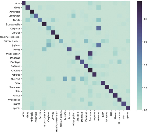
Figure 8. The average fluorescence spectrum data with standard deviation for Carpinus, Juglans, Quercus, and Taxaceae.

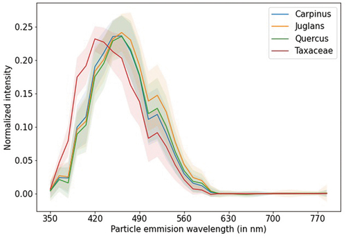
Figure 9. Precision, recall, and F1 score for each class (abbreviations defined in the Labeled dataset subsection).

Accurate classification is a prerequisite for application in the operational mode. However, it should be emphasized that because of flowering seasonality, all pollen types classified in this study never overlap. Therefore, the presented results are expected to underestimate the performance in the operational setup, as confirmed in previous studies (Matavulj et al. 2022; Simonyan and Zisserman 2015). From the end-user perspective, false positives are equally unwanted as false negatives, with particular importance to avoiding misclassifications at the beginning of the season when the cause and treatment of the first symptoms are to be determined. The uncertainty of classifications should be reported with the result, and additional quality control procedures suggested by Crouzy et al. (2022) could limit the number of misidentifications. It should be noted that for individual patients, the quantities measured at the usual monitoring locations (i.e., single point measurement at roof level) have limited value because the exposure takes place at street level and is not limited to a single location during the day. The real-time measurements are of utmost importance for atmospheric dispersion models as they allow improvements via data assimilation, and they can handle data coming with known uncertainty.

Conclusion

This paper evaluates more advanced architectures of CNNs for pollen classification on Rapid-E data and proposes a new model which, coupled with a specific training strategy, improves the current state-of-the-art. So far, vanilla CNNs are the only CNN types experimented for pollen classification on Rapid-E data (Boldeanu et al. 2021; Sauliene et al. 2019; Simonyan and Zisserman 2015). Therefore, we wanted to further contribute to the development of pollen classification models by adjusting more advanced concepts of CNNs, residual, and inception networks since they yielded better results on other datasets compared to vanilla CNNs (Krizhevsky, Sutskever, and Hinton 2012; Simonyan and Zisserman 2015). Although all tested models were expected to improve on the vanilla CNN since they yielded better results on other datasets, most of the models did not achieve that, implying that model implementation depends heavily on the data. However, residual networks improved over the vanilla CNNs for each data type (Table 2). We further showed that this is not the case for the multi-modal settings when learning starts from random weights. This is probably because the multi-modal ResNet has 5.6 times more parameters than a vanilla CNN, so learning new information from features of smaller spatial dimensions is more challenging when there are a lot of trainable parameters. However, when the pretrained weights of FEs are implemented from the models trained on each input separately, the multi-modal ResNet gains a boost and outperforms the vanilla CNN. To conclude, we have improved the current state-of-the-art with ResNets. Still, their use is not straightforward and requires adaptation and specific training strategies to surpass the vanilla CNNs on the examined pollen classification task.

Acknowledgments

We acknowledge support from COST Action CA18226 “New approaches in detection of pathogens and aeroallergens (ADOPT)” (www.cost.eu/actions/CA18226). This research was funded by the BREATHE project from the Science Fund of the Republic of Serbia PROMIS program, grant agreement no. 6039613, and by the Ministry of Education, Science and Technological Development of the Republic of Serbia, grant agreement no. 451-03-68/2022-14/200358. This research was supported by the RealForAll project (2017HR-RS151), co-financed by the Interreg IPA Cross-border Cooperation program Croatia – Serbia 2014-2020 and Provincial secretariat for finances, Autonomous Province Vojvodina, Republic of Serbia, contract no. 102-401-337/2017-02-4-35-8.

Disclosure statement

No potential conflict of interest was reported by the authors.

Additional information

Funding

The work was supported by the Ministry of Education, Science and Technological Development of the Republic of Serbia [451-03-68/2022-14/200358]; Science Fund of the Republic of Serbia [6039613].

References

- Beggs, P. J. 2017. Allergen aerosol from pollen-nucleated precipitation: A novel thunderstorm asthma trigger. Atmospheric environment 152:455–61. doi:10.1016/j.atmosenv.2016.12.045.
- Bennett, K. D., and K. J. Willis. 2002. Pollen. In Tracking environmental change using lake sediments. developments in paleoenvironmental research, J. P. Smol, H. J. B. Birks, W. M. Last, R. S. Bradley, and K. Alverson. ed., vol. 3, Dordrecht: Springer. 10.1007/0-306-47668-1\_2
- Boldeanu, M., H. Cucu, C. Burileanu, and L. Marmureanu. 2021. Multi-Input convolutional neural networks for automatic pollen classification. Applied Sciences 11 (24):11707. doi:10.3390/app112411707.
- Boldeanu, M., M. González-Alonso, H. Cucu, C. Burileanu, J. M. Maya-Manzano, and J. T. M. Buters. 2022. Automatic pollen classification and segmentation using u-nets and synthetic data. IEEE Access 10:73675–84. doi:10.1109/ACCESS.2022.3189012.
- Burbach, G. J., L. M. Heinzerling, G. Edenharter, C. Bachert, C. Bindslev-Jensen, S. Bonini, J. Bousquet, L. Bousquet-Rouanet, P. J. Bousquet, M. Bresciani, et al. 2009. GA2LEN skin test study II: Clinical relevance of inhalant allergen sensitizations in Europe. Allergy. 64(10):1507–15. doi:10.1111/j.1398-9995.2009.02089.x.
- Buters, J. T. M., C. Antunes, A. Galveias, K. C. Bergmann, M. Thibaudon, C. Galan, C. Schmidt-Weber, and J. Oteros. 2018. Pollen and spore monitoring in the world. Clinical and Translational Allergy 8 (1):9. PMID: 29636895; PMCID: PMC5883412. doi:10.1186/s13601-018-0197-8.
- Buters, J., B. Clot, C. Galán, R. Gehrig, S. Gilge, F. Hentges, D. O’Connor, B. Sikoparija, C. Skjoth, F. Tummon, et al. 2022. Automatic detection of airborne pollen: An overview. Aerobiologia. doi:10.1007/s10453-022-09750-x.
- Crouzy, B., G. Lieberherr, F. Tummon, and B. Clot. 2022. False positives: Handling them operationally for automatic pollen monitoring. Aerobiologia 38 (3):429–32. doi:10.1007/s10453-022-09757-4.
- Culley, T. M., S. G. Weller, and A. K. Sakai. 2002. The evolution of wind pollination in angiosperms. Trends in Ecology & Evolution 17 (8):361–69. doi:10.1016/S0169-5347(02)02540-5.
- Dahl, A., C. Galán, L. Hajkova, A. Pauling, B. Sikoparija, M. Smith, and D. Vokou. 2013. The onset, course and intensity of the pollen season. In Allergenic pollen: A review of the production, release, distribution and health impacts, ed. M. Sofiev and C.-K. Bergman, 29–70. pp272. Springer Verlag. doi: 10.1007/978-94-007-4881-1\_3.
- D’Amato, G., L. Cecchi, S. Bonini, C. Nunes, I. Annesi-Maesano, H. Behrendt, G. Liccardi, T. Popov, and P. van Cauwenberge. 2007. Allergenic pollen and pollen allergy in Europe. Allergy 62 (9):976–90. doi:10.1111/j.1398-9995.2007.01393.x.
- de Weger, L. A., P. T. W. van Hal, B. Bos, F. Molster, M. Mostert, and P. S. Hiemstra. 2021. Personalized pollen monitoring and symptom scores: A feasibility study in grass pollen allergic patients. Frontiers in Allergy 2:628400. doi:10.3389/falgy.2021.628400.
- He, K., X. Zhang, S. Ren, and J. Sun. 2016. Deep residual learning for image recognition. Proceedings of the 2016 IEEE Conference on Computer Vision and Pattern Recognition (CVPR). 770–78. doi: 10.1109/cvpr.2016.90
- Hirst, J. M. 1952. An automatic volumetric spore trap. The Annals of Applied Biology 39 (2):257–65. doi:10.1111/j.1744-7348.1952.tb00904.x.
- Hsiao, T. Y., Y. C. Chang, H. H. Chou, and C. T. Chiu. 2019. Filter-based deep-compression with global average pooling for convolutional networks. Journal of Systems Architecture 95:9–18. doi:10.1016/j.sysarc.2019.02.008.
- Huffman, J. A., A. E. Perring, N. J. Savage, B. Clot, B. Crouzy, F. Tummon, O. Shoshanim, B. Damit, J. Schneider, V. Sivaprakasam, et al. 2019. Real-time sensing of bioaerosols: Review and current perspectives. Aerosol Science and Technology. 54(5):1–56. doi:10.1080/02786826.2019.166472.
- Kasprzyk, I., B. Ortyl, and A. Dulska-Jez. 2014. Relationships among weather parameters, airborne pollen and seed crops of Fagus and Quercus in Poland. Agricultural and Forest Meteorology 197:111–22. doi:10.1016/j.agrformet.2014.05.015.
- Kawashima, S., B. Clot, T. Fujita, Y. Takahashi, and K. Nakamura. 2007. An algorithm and a device for counting airborne pollen automatically using laser optics. Atmospheric Environment, 41(36), 7987–7993. doi:10.1016/j.atmosenv.2007.09.019
- Krizhevsky, A., I. Sutskever, and G. E. Hinton. 2012. ImageNet classification with deep convolutional neural networks. Proceedings of the 2012 Advances in Neural Information Processing Systems 25 (NIPS). doi:10.1145/3065386.
- Larsson, G., M. Maire, and G. Shakhnarovich. 2016. FractalNet: Ultra-Deep Neural Networks Without Residuals doi:10.48550/arXiv.1605.07648.
- Matavulj, P., S. Brdar, M. Racković, B. Sikoparija, and I. N. Athanasiadis. 2021. Domain adaptation with unlabeled data for model transferability between airborne particle identifiers. 17th International Conference on Machine Learning and Data Mining (MLDM 2021), New York, USA. doi: 10.5281/zenodo.5574164
- Matavulj, P., A. Cristofori, F. Cristofolini, E. Gottardini, S. Brdar, and B. Sikoparija. 2022. Integration of reference data from different rapid-E devices supports automatic pollen detection in more locations. The Science of the Total Environment 158234. doi:10.1016/j.scitotenv.2022.158234.
- O’Connor, D. J., D. A. Healy, S. Hellebust, J. T. M. Buters, and J. R. Sodeau. 2014. Using the wibs-4 (waveband integrated bioaerosol sensor) technique for the on-line detection of pollen grains. Aerosol Science and Technology 48 (4):341–49. doi: 10.1080/02786826.2013.872768.
- Oteros, J., F. Orlandi, H. García-Mozo, F. Aguilera, A. B. Dhiab, T. Bonofiglio, M. Abicou, L. Ruiz-Valenzuela, M. Mar Del Trigo, C. Diaz de la Guardia, et al. 2014. Better prediction of Mediterranean olive production using pollen-based models. Agronomy for Sustainable Development 34:685–94. doi:10.1007/s13593-013-0198-x.
- Oteros, J., A. Weber, S. Kutzora, J. Rojo, S. Heinze, C. Herr, R. Gebauer, C. B. Schmidt-Weber, and J. T. M. Buters. 2020. An operational robotic pollen monitoring network based on automatic image recognition. Environmental Research 191:110031. doi:10.1016/j.envres.2020.110031.
- Plaza, M. P., F. Kolek, V. Leier-Wirtz, J. O. Brunner, C. Traidl-Hoffmann, and A. Damialis. 2022. Detecting airborne pollen using an automatic, real-time monitoring system: Evidence from two sites. International Journal of Environmental Research and Public Health 19 (4):2471. doi:10.3390/ijerph19042471.
- Sauliene, I., L. Šukienė, G. Daunys, G. Valiulis, L. Vaitkevičius, P. Matavulj, S. Brdar, M. Panic, B. Sikoparija, B. Clot, et al. 2019. Automatic pollen recognition with the rapid-E particle counter: The first-level procedure, experience and next steps, atmos. Atmospheric Measurement Techniques. 12(6):3435–52. doi:10.5194/amt-12-3435-2019.
- Sauvageat, E., Y. Zeder, K. Auderset, B. Calpini, B. Clot, B. Crouzy, T. Konzelmann, G. Lieberherr, F. Tummon, and K. Vasilatou. 2020. Real-time pollen monitoring using digital holography. Atmospheric Measurement Techniques 13 (3):1539–50. doi:10.5194/amt-13-1539-2020.
- Schiele, J., F. Rabe, M. Schmitt, M. Glaser, F. Haring, J. O. Brunner, B. Bauer, B. Schuller, C. Traidl-Hoffmann, and A. Damialis. 2019. Automated classification of airborne pollen using neural networks. 41st Annual International Conference of the IEEE Engineering in Medicine and Biology Society (EMBC). doi: 10.1109/embc.2019.8856910
- Sikoparija, B., P. Matavulj, G. Mimić, M. Smith, Ł. Grewling, and Z. Podrascanin. 2022. Real-time automatic detection of starch particles in ambient air. Agricultural and Forest Meteorology 323:109034. doi:10.1016/j.agrformet.2022.109034.
- Sikoparija, B., G. Mimic, P. Matavulj, M. Panic, I. Simovic, and S. Brdar. 2019. Short communication: Do we need continuous sampling to capture variability of hourly pollen concentrations? Aerobiologia 36 (1):3–7. doi:10.1007/s10453-019-09575-1.
- Simonyan, K., and A. Zisserman. 2015. Very deep convolutional networks for large-scale image recognition. Proceedings of The International Conference on Learning Representations (ICLR). 75, 6:398–406. doi: 10.48550/arXiv.1409.1556
- Sofiev, M. 2019. On possibilities of assimilation of near-real-time pollen data by atmospheric composition models. Aerobiologia 35 (3):523–31. doi:10.1007/s10453-019-09583-1.
- Sothe, C., C. M. De Almeida, M. B. Schimalski, L. E. C. La Rosa, J. D. B. Castro, R. Q. Feitosa, M. Dalponte, C. L. Lima, V. Liesenberg, G. T. Miyoshi, et al. 2020. Comparative performance of convolutional neural network, weighted and conventional support vector machine and random forest for classifying tree species using hyperspectral and photogrammetric data. GIScience & Remote Sensing. 57(3):1–26. doi:10.1080/15481603.2020.1712102.
- Srivastava, R. K., K. Greff, and J. Schmidhuber. 2015. Training very deep networks. In proceedings of the 2015 Advances in Neural Information Processing Systems (NIPS). doi: 10.48550/arXiv.1507.06228
- Szegedy, C., W. Liu, Y. Jia, P. Sermanet, S. Reed, D. Anguelov, D. Erhan, V. Vanhoucke, and A. Rabinovich. 2015. Going deeper with convolutions. 2015 IEEE Conference on Computer Vision and Pattern Recognition (CVPR). doi: 10.1109/cvpr.2015.7298594
- Szegedy, C., V. Vanhoucke, S. Ioffe, J. Shlens, and Z. Wojna. 2016. Rethinking the inception architecture for computer vision. 2016 IEEE Conference on Computer Vision and Pattern Recognition (CVPR). doi:10.1109/cvpr.2016.308
- Tesendic, D., D. Boberic-Krsticev, P. Matavulj, S. Brdar, M. Panic, V. Minic, and B. Sikoparija. 2020. RealForall: Real-time system for automatic detection of airborne pollen. Enterprise Information Systems 16 (5). doi:10.1080/17517575.2020.1793391.
- Tummon, F., S. Adamov, B. Clot, B. Crouzy, M. Gysel-Beer, S. Kawashima, G. Lieberherr, J. Manzano, E. Markey, A. Moallemi, et al. 2021. A first evaluation of multiple automatic pollen monitors run in parallel. Aerobiologia. doi:10.1007/s10453-021-09729-0.
- Viertel, P., and M. König. 2022. Pattern recognition methodologies for pollen grain image classification: A survey. Machine Vision and Applications 33 (1):18. doi:10.1007/s00138-021-01271-w.
- Xie, S., R. Girshick, P. Dollar, Z. Tu, and K. He. 2017. Aggregated residual transformations for deep neural networks. Proceedings of the 2017 IEEE Conference on Computer Vision and Pattern Recognition (CVPR). doi: 10.1109/cvpr.2017.634
- Zagoruyko, S., and N. Komodakis. 2016. Wide residual networks. Proceedings the British Machine Vision Conference .87.1–12. doi:10.48550/arXiv.1605.07146.
- Ziska, L., K. Knowlton, C. Rogers, D. Dalan, N. Tierney, M. A. Elder, W. Filley, J. Shropshire, L. B. Ford, C. Hedberg, et al. 2011. Recent warming by latitude associated with increased length of ragweed pollen season in central North America. Proceedings of the National Academy of Sciences. 108(10):4248e4251. doi:10.1073/pnas.1014107108.